Osteoporosis Recognition
Based on Similarity Metric with SVM
Ke Zhou1, Jie Cai1,#, Yong-Hui Xu2, Tian-Xiu Wu3,* 1School of Information Engineering
Guangdong Medical University Zhanjiang 524023, China
E-mails: [email protected], [email protected], [email protected]
2School of Computer Science and Engineering
South China University of Technology Guangzhou 510006, China
E-mail: [email protected]
3School of Basic Medical Science
Guangdong Medical University Zhanjiang 524023, China E-mail: [email protected]
#Author contributed equally to the paper *Corresponding author
Received: January 11, 2016 Accepted: June 1, 2016
Published: June 30, 2016
Abstract: The purpose: Applying different techniques of classification to osteoporotic bone tissue texture analysis, exploring the recognition rate of the different classification methods.
Methods: Using gray-level co-occurrence matrix (GLCM) and running a length matrix texture analysis to extract bone tissue slice image characteristic parameters, and to classify respectively 4 and 10 microscope images of the two groups: the sham (SHAM) and the ovariectomized (OVX) group image.
Results: The metric support vector machine (SVM) classification algorithm, based on SVM learning or recognition rate, was higher than the stand-alone measure, and the classification results were stable.
Conclusion: Measurement of the SVM classification algorithm for osteoporotic bone slices texture analysis revealed a high recognition rate.
Keywords: Osteoporosis, Texture analysis, Information-theoretic metric learning (ITML), Support vector machine (SVM).
Introduction
The World Health Organization (WHO) defines osteoporosis as “the system for metabolic bone diseases”, with characteristics of “low bone mass” and “degeneration of bone
microarchitecture”, which leads to increasing osteopsathyrosis [12]. This definition
emphasizes the bone mass, paying more attention to the quality of the bones, such as the microarchitecture of the bones. The definition of bone microarchitecture is the connection degree between the three-dimensional construction of bone trabecular and the trabecular. The bone trabecular are highly complex, anisotropic materials, which could bear the different sized tensile and compressive stresses [13]. Studying the anisotropy of the bone trabecular is the key to the accuracy of the biomechanical analysis [6, 11], which reflects the problems of the consistency of bone trabecular. Similarly, compared with the bone mineral density (BMD), which would be the determinant of the osteopsathyrosis [1, 8], the changes of trabecular microarchitecture are more sensitive. The traditional bone histomorphometry is one of the gold standards in quantitative analysis of bone microarchitecture [9]. On account of the principles of stereology, this method utilizes the two-dimensional image to calculate the related parameters of bone microarchitecture, which would observe and measure scientifically, the morphological changes of the quality level of bone tissue (bone structure) and the quantity (bone mass) [3]. Due to the drifting structural pattern of bones [15], traditional bone histomorphometry cannot determine the anisotropic structure, because it is difficult to reflect the stereo-chemical structure of the bone trabecular. However, the morphometry of the two-dimensional biopsy could obtain the kinetic parameters of the bone tissues, which would provide the dynamic information of the bone histology regarding the bone remodeling and construction. All of these parameters could not be achieved by the morphometry of a three-dimensional biopsy unless an invasive computed tomographic (CT) microscope were used. The use of the micro CT and magnetic resonance imaging (MRI) have been limited by the various imaging conditions, using the standard contradictions and the expensive cost. These machines have determined that bone histomorphometry is an irreplaceable field of research with many clinical applications. On that account, based on bone histomorphometry, exploring a more convenient and objective technological means that can better evaluate bone trabecular anisotropic characteristics is the most important area of study in the osteoporosis field.
The image processing techniques were used to extract the texture characteristic parameters and the quantitative or qualitative description. From this, the texture analysis could analyze the image in the region of the image (many pixels). Image texture analysis has been widely used in medical imaging, especially for the image processing of MRIs of the brain [7, 18]. Also, some scholars have incorporated texture analysis into the imaging diagnosis of osteoporosis [10, 16], but do not involve it in the field of bone histomorphometry. According to the previous research [17], texture analysis could distinguish between rats with osteoporosis, without the ovary and bone tissue, and normal rats, which demonstrates it as an effective analysis technique. At the same time, under the four-time mirror, regions of interest (ROI) were extracted (Fig. 1), and then the texture features at the ROI area of 0°, 45°, 90°,
135° were extracted by choosing the co-occurrence and run-length matrix methods. The results in [2] show that there are significant differences in the texture parameters between the rats with osteoporosis, without ovary and bone tissue, and the normal rats (p < 0.05). Based on previous studies, the research obtained the texture characteristics by using the co-occurrence and run-length matrix, and then classified the texture characteristics according to the different classification techniques to discuss the recognition rate of different algorithms.
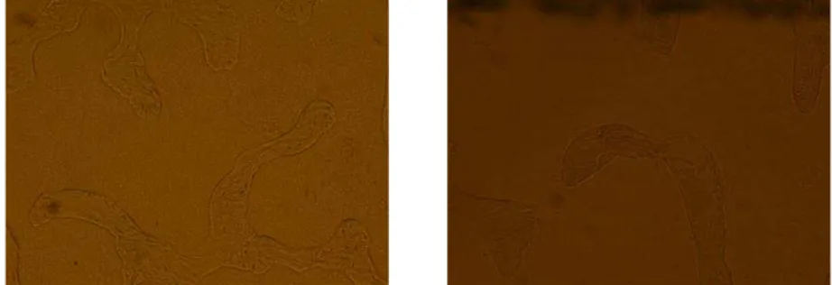
Fig. 1 Normal biopsy samples (left) and OVX slice (right) under 4 magnification
Fig. 2 Normal biopsy samples (left) and OVX slice (right) under 10 magnification
Materials and methods
Animals for the experiment and data sources
Table 1. Data sample case
Group Microscope 4 Microscope 10
SHAM 16 47
OVX 11 40
Classical classification algorithms
Support vector machine
SVM aims to find an optimal hyper plane to minimize global structural risk [4, 14]. This hyper plane can be represented as w x bT 0, where:
* * 2
2
( , ) 1
T
1
( , ) arg min || ||
2
. . , ( ) 1 , 0
n p i
w b i
i i i i
w b w C
s t i y w x b
. (1)Currently, within the existing classification algorithms, SVM is the most suitable algorithm for solving binary classification problems, especially in the case of small, nonlinear and highly dimensional samples.
Due to the fact that SVM has a strong generalization capability, it is the most commonly used classification algorithm in many practical applications. This is also the basic motivation for us to choose SVM as the base classification algorithm.
SVMs have been researched and documented thoroughly in the literature. For the classification of small samples, the authors found that tested linear SVM (Linear-SVM) classification to be the best method. Therefore, in this paper, the results provided only Linear-SVM for classification.
Metric learning
Metric learning is an important branch of machine learning. It is used to calculate a metric space which can minimize the distance within the class and maximize the distance between classes.
Given a transformation matrix L, the mahalanobis distance between xi and xj can be represented as:
T T T
( , ) ( ) ( )
L i j i j i j
S x x Lx Lx x L Lx (2)
The learning transformation matrix L is equivalent to the learning mahalanobis matrix
T
M L L.
If A1 is replaced by A2, the distribution will change. The KL-divergence between distributions generated by A1 and A2can be represented as:
1
1 2 1
2
( ; , )
( ( ; , ) || ( ; , )) ( ; , ) log
( ; , )
p x m A KL p x m A p x m A p x m A dx
p x m A
. (3)The optimal metric space generated by A can be minimized KL p x m A( ( ; , ) || ( ; ,p x m A0)). When calculated, A is equivalent to the minimum D A A( ,1 2), where:
T
( , ) ( ) ( ) ( ) ( )
D x y x y x y y . (4)
The ITML algorithm is described as follows: Algorithm: ITML
Input: XRd n* , S: Collection of pair points within class, D: Collection of pair points between classes, e: Threshold
Output: W
1. Assume W0 Id, and ij 0, i j,
2. While |Wt Wt1|e:
For ( ,x xi j) in S or D
Compute w(xixj)T
if ( ,x xi j)S :
2 2
1 1
min ,
|| ||
ij
w u
2
2
/ 1 ||w||
Else if ( ,x xi j)D
2 2
1 1
min ,
|| ||
ij
l w
2
2
/ 1 ||w||
ij ij
Compute Cholesky-decomposition: LLT I wwT
Wt L WT t1
3. Return W
Support vector machine based on metric learning
Linear-SVM was proposed in [19]. The basic motivation is to combine metric learning with SVM.
* * * 2 2 2 2
( , , ) 1
T
1
( , , ) arg min ( ) || ||
2
. . , ( ) 1 , 0
n
i
L w b i
i i i i
L w b R L w C
s t i y w Lx b
, (5)where L* is the optimal metric and (w b*, *) is the optimal hyper plane.
This optimization problem can be solved by gradient descent:
1 | ,t 1 | ,t 1 [ | ]t
t t w t t w t t w
f f f
w w b b L L
w b L
, (6)
where:
T
1
2 max 0, 1 ( )
n
i i i i
i
f
w C y w Lx b y Lx
w
,1
2 max 0, 1 ( )
n
T
i i i
i
f
C y w Lx b y b
, (7)
T T
1
2 max 0, 1 ( )
n
i i i i
i
f
C y w Lx b y wx L
.Linear Metric learning with SVM (L-MSVM) algorithm is described as follows:
Algorithm: L-MSVM Input: Dataset:{ , }n 1
i i i
x y
Output: * * *
, ,
L w b
Initial: 6 0 0 0
1
1
(0 1), 10 , , , ,
n
i i i
i
e x x x L w b n
for t0, 1, 2,
Calculate gradient
( ,t t, t)
f L w b
by Eq. (7)
for m0, 1, 2, m
Update (Lt1, wt1,bt1) by Eq. (6)
If Armijo condition is satisfied: break
if ( , , ) ( 1, 1, 1)
| |
( , , )
t t t t t t
t t t
f L w b f L w b
f L w b
,
* *
1, * 1, 1
t t t
L L w w b b
break
Results and discussion
15 characteristic parameters were obtained, such as entropy, contrast, and factors and so on. Then, the two-samples were used to screen significant differences from two sets of 15 parameters. T-test selection parameters, as well as specific differences in the number of parameters, are as shown in Table 2.
Table 2. Parameters showing differences
Group (number) Parameter
Group 4 (13)
Angular second moment, contrast, square and deficit moments, and variance, entropy, and entropy, difference entropy, run length nonuniformity factor, difference variance, intensity inhomogeneity factor, long-run factors, short-run factors
Group 10 (6) Deficit moment, sum entropy, entropy,
difference entropy, short run factor
To study the combined results of different classification algorithms, the experimental data was grouped. In the first experiment, after obtaining the filtered texture parameters, the three methods of linear SVM, ITML and L-MSVM were used directly to classify 10 times without a screening phase. Fig. 3 shows the results obtained:
Fig. 3 The classified results without selection feature parameters
From Figs. 3 and 4, it is clear that the classification accuracy based upon SVM measurement technology was the highest and most stable. The accuracy of just SVM and ITML was relatively lower and the experimental results were volatile.
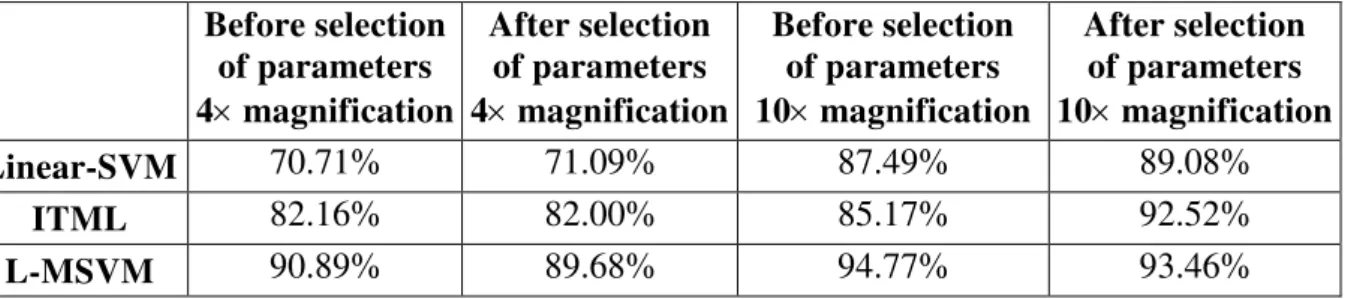
Table 3 shows the mean value of the classification results before and after the selection of the characteristic parameters.
Table 3. The mean value for each experiment 10 times
Before selection of parameters 4 magnification
After selection of parameters 4magnification
Before selection of parameters 10magnification
After selection of parameters 10magnification Linear-SVM 70.71% 71.09% 87.49% 89.08%
ITML 82.16% 82.00% 85.17% 92.52%
L-MSVM 90.89% 89.68% 94.77% 93.46%
As can be seen from Table 3, the overall accuracy rate of the results of the classification parameters under 4 magnification was lower than the result obtained under 10 magnification. In the four experiments of the three methods, the accuracy rate of the SVM classification algorithm based on the metrics was highest.
Another study of this experiment was to compare whether the image feature selection had a direct impact on the classification results. As can be seen from Table 3 and Fig. 4, the classification results from before and after the selection under 4 magnification did not exhibit great difference. However, after feature selection under 10 magnification, the recognition rate of Linear-SVM and ITML improved greatly. The author believes that 4 magnification, which before the feature selection had 15 parameters and after feature selection had only 13 parameters, showed that the number of parameters after the recognition rate was not very different. Conversely, while under 10 magnification, before feature selection it had 15 parameters, and after selection there were only six parameters which shows that there were significantly different characteristics after the selection. Therefore, the recognition rate after the selection of two algorithms improved significantly. Using the L-MSVM algorithm, the recognition rate of both before and after feature selection or selection feature, was very high, indicating that the degree of difference between the characteristic parameters for the algorithm was not sensitive and is reliable.
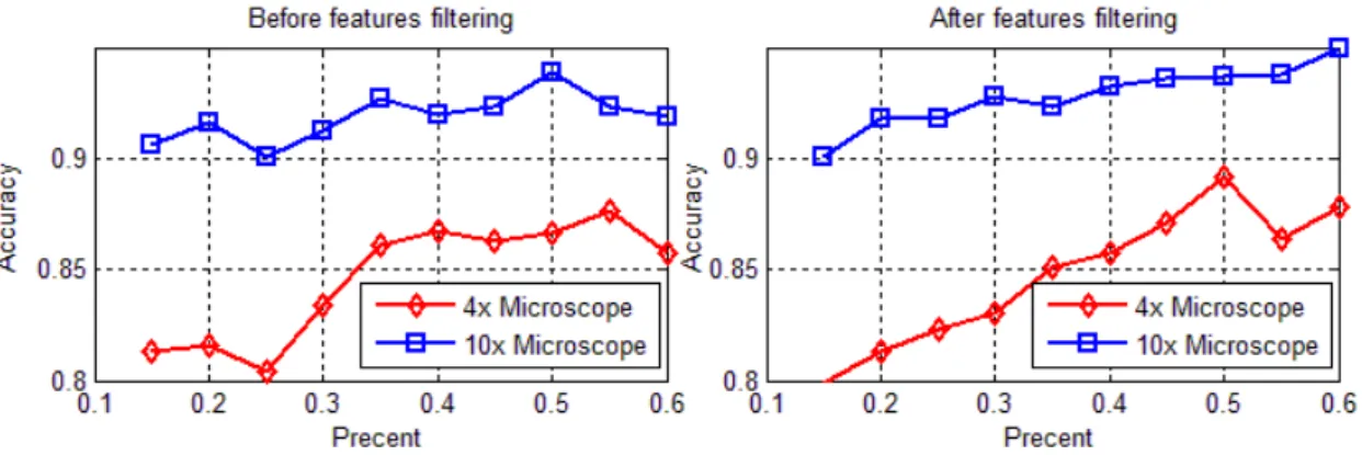
Fig. 5 The results of training samples of different proportion
As can be seen from Fig. 5, as the proportion of the samples increased, the recognition rate also gradually increased. When the proportion of the training samples was about 50%, the recognition rate was maximized and, as can be seen from Fig. 5, the recognition rate under 10 magnification was higher than under 4 magnification. Before no feature selection, the recognition rate curve fluctuated whilst after feature selection, the recognition rate curve was steadily increasing. Thus, feature selection for sample classification still plays a certain role.
Conclusion
In this study, the analysis for the different classification algorithms of osteoporosis can be seen. The recognition rate based on a measure was higher than a SVM algorithm using just learning metrics or SVM, and the classification results are more stable. On the other hand, as can be seen from the two sets of experiments, even if there was no filter for texture parameters, a high recognition rate could be still be obtained. Thus, we can conclude that, a SVM classification algorithm based on the metrics is suitable for low-dimensional, small sample data classification.
The image feature selection has a direct impact on the classification results. For the L-MSVM algorithm, the recognition rate of both before and after feature selection or selection feature was very high, indicating that the degree of difference between the characteristic parameters for the algorithm was not sensitive but was more robust.
The SVM classification algorithm based metrics can be used in the diagnosis of osteoporosis bone slice texture, thus it had a guiding significance in the diagnosis results on the limited conditions of medical experiments and clinical cases.
Acknowledgements
This study was supported by National Natural Science Foundation of China (No. 81541104), Science and Technology Project of Guangdong Province (No. 2014A030304006), Science and Technology Project of Zhanjiang (No. 2015A01039).
References
1. Brandi M. L. (2009). Microarchitecture, the Key to Bone Quality, Rheumatology (Oxford) 2009, 48(4), iv3-8.
3. Chen J., H. Zhang, G. Yang, X. Lu, X. Jin, L. Lu, Q. Li (2014). Expert Consensus about the Current Application of Bone Histomorphmetry, Chinese Journal of Osteoporosis, 12(10), 1031-1038 (in Chinese).
4. Cortes C., V. N. Vapnik (1995). Support Vector Networks, Mach Learn, 20, 273-297. 5. Davis J., B. Kulis, P. Jain, S. Sra, I. S. Dhillon (2007). Information-theoretic Metric
Learning, Proc 24th Int Conf Mach Learn, 209-216.
6. Hazrati Marangalou J., K. Ito, B. van Rietbergen (2015). A Novel Approach to Estimate Trabecular Bone Anisotropy from Stress Tensors, Biomech Model Mechanobiol, 14(1), 39-48.
7. Hu L.-J., X. Li, H. Xia, L-Z. Tong (2012). 3D Texture Analysis of Hippocampus based on MR Images in Patients with Alzheimer Disease and Mild Cognitive Impairment, Journal of Beijing University of Technology, 38(6), 942-947 (in Chinese).
8. Koehne T., E. Vettorazzi, N. Küsters, R. Lüneburg, B. Kahl-Nieke, K. Püschel, M. Amling, B. Busse (2014). Trends in Trabecular Architecture and Bone Mineral Density Distribution in 152 Individuals Aged 30-90 Years, Bone, 66, 31-38.
9. Li Q. (2001). The Study of Animal Experiment on Osteopeina-bone Histomorphometry, Sichuan University Press (in Chinese).
10.Ollivier M., T. Le Corroller, G. Blanc, S. Parrattea, P. Champsaura, P. Chabranda, J.-N. Argensona (2013). Radiographic Bone Texture Analysis is Correlated with 3D Microarchitecture in the Femoral Head, and Improves the Estimation of the Femoral Neck Fracture Risk when Combined with Bone Mineral Density, Eur J Radiol, 82(9), 1494-1498.
11.Pei B.-Q., T.-M. Wang (2008). Comprehensive Biomechanical Analysis of Microcosimc Trabecular Structure of Cancellous Bone, Journal of Beijing University of Aeronautics and Astronautics, 34(2), 215-218 (in Chinese).
12.Qi J., H.-F. Xu, J. Wang et al. (2012). Application of Bone Histomorphometry and Micro CT Measurement Technology in the Study of Osteoporosis, International Journal of Orthopaedics, 33(3), 157-159 (in Chinese).
13.Udhayakumar G., C. M. Sujatha, S. Ramakrishnan (2013). Trabecular Architecture Analysis in Femur Radiographic Images Using Fractals, Proc Inst Mech Eng H, 227(4), 448-453.
14.Vapnik V. N. (1995). The Nature of Statistical Learning Theory, New York: Springer-Verlag.
15.Wang H. (2009). Drug Research Methods and Technology in Osteoporosis, Beijing People’s Medical Publishing House, 134 (in Chinese).
16.Wolski M., P. Podsiadlo, G. W. Stachowiak (2014). Directional Fractal Signature Methods for Trabecular Bone Texture in Hand Radiographs: Data from the Osteoarthritis Initiative, Medical Physics, 41(8), doi: 10.1118/1.4890101.
17.Wu T., J. Cai (2014). Quantitative Diagnosis of Osteoporosis based on Texture Analysis, Chinese Journal of Osteoporosis, 20(7), 10-14 (in Chinese).
18.Zhou K., J. Cai, G.-Q. Xiong (2014). Optimized VBM and DARTEL Algorithm in Analyzing MRI of Alzheimer’s Disease, Chin J Med Imaging Technol, 30(3), 462-466 (in Chinese).
Assoc. Prof. Ke Zhou, M.Sc.
E-mail: [email protected]
Ke Zhou is an Associate Professor. She had her major in Computer Application. Now she is engaged in the researches on medical data mining and medical image analysis and processing.
Jie Cai, M.Sc.
E-mail: [email protected]
Jie Cai is a lecturer. She had her major in Applied Mathematics. Now she is engaged in the researches on medical data mining and medical image analysis and processing.
Yong-Hui Xu, Ph.D. Student
E-mail: [email protected]
Assoc. Prof. Tian-Xiu Wu, M.Sc.
E-mail: [email protected]