Time series forecasting for a call center in a Warsaw holding company

(1)

i

Dominika Leszko

Internship report presented as partial requirement for

obtaining the Master’s degree in Data Science and Advanced

Analytics

Time Series Forecasting for a Call Center

in a Warsaw Holding Company

Time Series Forecasting for a Call Center

in a Warsaw Holding Company

(2)

2

NOVA Information Management School

Instituto Superior de Estatística e Gestão de Informação Universidade Nova de Lisboa

TIME SERIES FORECASTING FOR A CALL CENTER IN A

WARSAW HOLDING COMPANY

by

Dominika Leszko

Internship report presented as partial requirement for obtaining the Master’s degree in Data Science and Advanced Analytics

Supervisor: Flavio Pinheiro

External Supervisor: Pawel Brach

(3)

3

ABSTRACT

In recent years, artificial intelligence and cognitive technologies are actively being adopted in industries that use conversational marketing. Workforce managers face the constant challenge of balancing the priorities of service levels and related service costs. This problem is especially common when inaccurate forecasts lead to inefficient scheduling decisions and in turn result in dramatic impact on the customer engagement and experience and thus call center’s profitability. The main trigger of this project development was the Company X’s struggle to estimate the number of inbound phone calls expected in the upcoming 40 days. Accurate phone call volume forecast could significantly improve consultants’ time management, as well as, service quality. Keeping this goal in mind, the main focus of this internship is to conduct a set of experiments with various types of predictive models and identify the best performing for the analyzed use case. After a thorough review of literature covering work related to time series analysis, the empirical part of the internship follows which describes the process of developing both, univariate and multivariate statistical models. The methods used in the report also include two types of recurrent neural networks which are commonly used for time series prediction. The exogenous variables used in multivariate models are derived from the Media Planning department of the company which stores information about the ads being published in the newspapers. The outcome of the research shows that statistical models outperformed the neural networks in this specific application. This report covers the overview of statistical and neural network models used. After that, a comparative study of all tested models is conducted and one best performing model is selected. Evidently, the experiments showed that SARIMAX model yields best predictions for the analyzed use-case and thus it is recommended for the company to be used for a better staff management driving a more pleasant customer experience of the call center.

KEYWORDS

Machine learning; Time Series Analysis; ARIMA; Forecasting; Supervised Learning; Predictive Models; Artificial Neural Networks; Recurrent Neural Networks; Gated Recurrent Unit; Long Short Term Memory;

(4)

4

LIST OF FIGURES

Figure 1: Trend Component of Time Series ... 13

Figure 2: Cyclical Component of Time Series. ... 13

Figure 3: Seasonal Component of Time Series. ... 14

Figure 4: Additive and Multiplicative Seasonality. ... 15

Figure 5: Examples of ACF and PACF plots and interpretations. ... 16

Figure 6: Model Complexity Bias-Variance Tradeoff. ... 19

Figure 7: Walk forward cross-validation technique with window size of one and four ... 21

Figure 8: Examples of data from autoregressive models with different parameters. ... 25

Figure 9: Examples of data from autoregressive models with different parameters ... 26

Figure 10: Recurrent Neural Network Loop ... 31

Figure 11: LSTM Memory Cell ... 32

Figure 12: Gated Recurrent Unit Cell ... 33

Figure 13: Univariate Dataset Distribution. ... 39

Figure 14: Time Series Component Decomposition. ... 40

Figure 15: Residuals of original time series. ... 41

Figure 16: Residuals of log-transformed time series. ... 41

Figure 17: Residuals of Square Root-transformed time series. ... 41

Figure 18: Residuals of Box Cox-transformed time series. ... 42

Figure 19: Rolling Mean and Standard Deviation over raw data series. ... 42

Figure 20: Rolling Mean and Standard Deviation over transformed data series. ... 43

Figure 21: Autocorrelation and Partial Autocorrelation plots. ... 46

Figure 22: Autocorrelation and Partial Autocorrelation plots on 1st order differenced data. .. 47

Figure 23: Manually defined model summary. ... 48

Figure 24: Automatically defined model summary. ... 48

Figure 25: Model diagnostics plots. ... 49

Figure 26: Gini feature importance bar plot. ... 52

Figure 27: Predictive accuracy of univariate and multivariate SARIMA(X) models. ... 54

Figure 28: GRU Base model architecture visualization. ... 57

Figure 29: GRU Base Model predictions over real data for train and test sets. ... 57

Figure 30: GRU Final Model predictions over real data for train and test sets. ... 63

(7)

7

LIST OF TABLES

Table 1: Results of Dickey-Fuller test on raw data. ... 44

Table 2: Results of Dickey-Fuller test on log-transformed data. ... 44

Table 3: Backward elimination results for SARIMAX vs Base Model. ... 53

Table 4: GRU parameter tuning: GRU nodes. ... 59

Table 5: GRU parameter tuning: Batch Size. ... 60

Table 6: GRU parameter tuning: Sequence length. ... 60

Table 7: GRU parameter tuning: Learning Rate. ... 61

Table 8: GRU parameter tuning: Layer Setup. ... 62

Table 9: LSTM parameter tuning: LSTM nodes. ... 65

Table 10: LSTM parameter tuning: Batch Size. ... 65

Table 11: LSTM parameter tuning: Sequence Length. ... 66

Table 12: LSTM parameter tuning: Learning Rate. ... 66

(8)

8

1. INTRODUCTION

In recent years, call centers have been revolutionized by the data. Even though some static one-size-fits-all strategies, as well as, static call scripts still remain, technology has changed significantly the way that call centers are functioning. The power of call centers remains in the huge amounts of data that such institutions gather when interacting with customers. It is possible for call center agents to know yet before receiving the call many crucial characteristics of the customer, such as which advertisement he has seen, what age range he falls into and what is his expenditure tendency. Naturally, as the time passes by, the customer database becomes larger and finally powerful enough to enable the call center to leverage all available data and drive appropriate interaction with each customer. American Express proved that 78 % of consumers have resigned from making an intended purchase due to poor customer service experience (2017, American Express Barometer). This is a clear sign that call centers must direct their focus onto a seamless and convenient experience for customers, unless they are ready to risk losing out on a competitor. To ensure that such scenario does not happen, more and more call centers are turning to technologies, such as Artificial Intelligence, Machine Learning and Time Series Analysis in order to provide them with useful insights. Layering in AI can include call volume forecast for better resource management or customer churn to determine appropriate marketing strategies, next best action, and more. Below report will present one of many possible applications of Statistical and Machine Learning methodologies aiming at improvement of operational efficiency in the life cycle of a Call Center.

1.1. PROJECT DESCRIPTION

At the second year of the NOVA IMS master program in Data Science and Advanced Analytics, I have enrolled in the internship program at a Holding Company (Company X) in Warsaw, Poland. The below report is a summary of the analytic activities developed by me as an intern during that period. During the internship, I joined the analytical team, which was mainly in charge of providing data visualizations in the form of BI dashboards, performing ETL processes and building a reliable Data Warehouse.

The main focus of my work was to identify Machine Learning opportunities within the umbrella of organizations to improve and automate the decision making processes. After throughout analysis of possible AI implementations and a number of discussions with business decision makers within the company, it has been agreed that the biggest need for automated optimization is currently laying in the subsidiary company providing Call Center service. More

(9)

9 specifically, the main challenge that the Call Center is currently facing is the consultants’ inefficient time management. Since the number of inbound phone calls is very unexpected, current call load balancing proves to be inefficient, often leading to either inactive at work agents as phone call frequency drops, or, on the other hand, insufficient number of calling agents at peak times. The latter often leads to dissatisfaction of customers caused by extended waiting time to be served by the consultant. This problem was previously attempted to be tackled within the company by means of a simple estimation that the phone call volume at the X following time steps would be equal to its average of X proceeding days. This solution did not result in a satisfactory accuracy, neither did it take advantage of the data stored at the Media Planning section of the company. This being said, the company’s solution leaves a lot of room for improvement given the relatively poor prediction quality. Last but not least, it is worth mentioning that accurate predictions of the inbound phone calls will bring value to not only the Call Center itself, but also, to the Supply Stock Management, as well as, Delivery Management Teams, which will have a better idea on which days more products will need to be available in stock for shipping.

Finally, in the work reported in this document, we aimed to combine business know-how and data engineering practices to gain the best prediction possible of the number of inbound phone calls for each of the next upcoming 40 days. Ultimately, we aimed to generate a series of predictions of customers’ responses to press-published advertisements of dietary supplements with the use of provided data that was collected by the company in the last 2 years. As aforementioned, accurate predictions would help in different areas of company’s activities, such as Delivery, Supply Stock Management and foremost in the Call Center’s staff time management, ultimately leading to a better Customer Experience and to a better company’s image in the market. Last but not least, another objective of the internship was to make a thorough and diversified research of the most optimal model for the analyzed use-case, including univariate and multivariate models, statistical models and recurrent neural networks.

1.2. BUSINESS CONTEXTUALIZATION

The work described in this report was developed during an internship in a Holding Company (Company X), consisting of an umbrella of brands, such as marketing agency, call center agency, logistics provider, software house, financial services provider, beauty service and employment agency.

(10)

10 The company contains rich and diverse data sources describing entire Path-To-Purchase of the customer, as he is targeted with marketing campaigns both online and in the press all the way to the moment when the product is delivered to him. In the present report, the focus is directed to the inbound phone calls from press advertisements aiming to increase the sale volume of dietary supplements. Such predictions will further contribute to primarily better staff management within the Call Center aiming at improvement of User Experience.

The data used in the work described in this report has been anonymized. We could not track any data to specific people, nor did we have access to any personal or sensitive information of the clients.

1.3. STRUCTURE OF THE PRESENT REPORT

The next chapter (Chapter 2 – theoretical framework) contains a theoretical summary of the methodology of algorithms used in this work (ARIMA, SARIMA, SARIMAX, GRU, LSTM). Further, chapter 3 (Chapter 3 – Related work) is dedicated to review the related work previously performed in a wide range of applications which make use of time series analysis methodology. This is followed by chapter 4 (Chapter 4 – Experiments and discussion) which describes the empirical part of this work, i.e. tested forecasting approaches and its results. Finally, the last chapter (Chapter 5) includes general conclusion, reflection on the limitations and suggestions for future work towards further improvement of the model.

(11)

11

2. THEORETICAL FRAMEWORK

2.1. TIME SERIES ANALYSIS

2.1.1. Introduction to Time Series

The term “Time series” relates to a data format consisting of the two main components: a time unit and a value or values associated with that particular time unit. What differs a time series from a standard dataset, time does not stand for just a metric, but it serves as a primary axis. A time series can be stored in two fundamental ways. One of them is to record a time series intervals as discrete points. These points can also represent other values which were measured for that specific timestamp and might occur in a periodic manner. Such time series are known as discrete time series. Financial or economical time series is a good example of a discrete time series, as usually various attributes are recorded on particular time intervals. Storing the values continuously along the time axis stands for the alternative way of recording a time series. Some examples of such time series include sensor data streamed from various Internet Of Things devices recording the data in a continuous manner.

2.1.2. Time Series Classification Types

Time series can be classified according to different attributes, one of which is a classification based on the stationarity. A feature which exhibits a change in mean, variance and time covariance is defined as stationarity. When it comes to the time series classification based on its stationarity, we can distinguish two categories:

- Stationary Time Series – A stationary time series has the property that the mean, variance and autocorrelation structure remain approximately constant over time. Stationarity can be defined in precise mathematical terms, but for this work purpose it can be considered as a flat looking series, not exhibiting any upward nor downward trend, with a constant and autocorrelation structure over time and with no periodic fluctuations (seasonality).

- Non-stationary Time Series - contrary to the stationary time series, it exhibits some non-flat patterns containing trend, seasonality, non-constant mean, variance or time covariance. In reality, great majority of time series are mostly categorized as non-stationary. Since a big number of time series techniques assumes stationarity of the data, some data pre-processing is often required before moving onto a forecasting phase.

(12)

12 Another kind of classification possible for a time series data is a classification based on a dependency between a new recorded value and its past values. Such classification results in two types of values:

- Long-Term memory time series – A typical characteristic of a long-term memory time series is slowly decreasing autocorrelation at consecutive lags in the autocorrelation function. In other words, it means that current values have high and significant correlations with a relatively large set of lags in the series. This property has been observed in both, financial series, as well as, stationary meteorological and environmental series, such as temperature change in the atmosphere, where today’s day temperature can be reconstructed by a large change of historic date temperatures. - Short-Tem memory time series – Unlike long-term memory time series, these exhibit a

fast, exponential decrease in the autocorrelation function, meaning that correlation between current value falls dramatically fast in the successive lags of the time series. Some typical examples of short-term memory series include econometric processes.

2.1.3. Time Series Components

One of primary goals of a time series analysis is to detect trends and other repeating patterns that occur over time. After correct identification and removal of the pattern, the remainder of the data should appear as a random, stable process with a chance variation, i.e. it should comply with the concepts of the previously described time series stationarity. The search of these patterns can be accomplished by relatively sophisticated statistical analyses, however, simple time plots are often capable of revealing the underlying patterns.

A key to analyzing a time series is to understand the form of any underlying pattern of the data ordered over time. This pattern potentially consists of several different components, all of which combine to yield the observed values of the time series. A time series analysis can isolate each component and quantify the extent to which each component influences the form of the observed data. If one or more individual components of a time series are isolated and identified, a forecast can project the underlying pattern into the future. (David Gerbing, 2016).

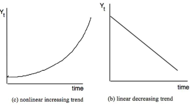
The first component of a time series is known as a trend and takes a form of a long-term growth or decline. A trend can be linear or nonlinear, which has been visualized in the figure below.

(13)

13

Figure 1: Trend Component of Time Series (David Gerbing, 2016)

The second component in the time series is called cyclical component. This pattern exists when data rises or falls do not happen over a fixed period. The duration of cyclical fluctuations is usually at least 2 years long. Cyclical pattern can be seen in a form of cyclical or long periodical rises and falls on a typical trend line. Due to the fact that this component is exhibited in as long time intervals as years or even decades, it is not common to see it in practical time series.

Figure 2: Cyclical Component of Time Series. (David Gerbing, 2016)

The third and last component of a time series is a seasonal component. This pattern can be seen in the form of short but repetitive fluctuations across the trend line. Seasonality is a relatively common aspect in the time series and can be often found in e.g. sales volume across time.

(14)

14 Figure 3: Seasonal Component of Time Series. (David Gerbing, 2016)

2.1.4. Types of Time Series Models

There are two commonly known types of time series models, which are differentiated according to the way that the time series components interact with each other:

- Additive models – Synthetically, these are the models, in which the effects of individual components are added together in order to model the underlying process. In other words, the behavior is linear and the values change consistently over time by the same amount, like e.g. linear trend. In such case, linear seasonality would imply same amplitude and frequency. This model can be represented by:

𝑌(𝑡) = 𝑇𝑟𝑒𝑛𝑑 + 𝑆𝑒𝑎𝑠𝑜𝑛𝑎𝑙 𝐶𝑜𝑚𝑝𝑜𝑛𝑒𝑛𝑡 + 𝐶𝑦𝑐𝑙𝑖𝑐𝑎𝑙 𝐶𝑜𝑚𝑝𝑜𝑛𝑒𝑛𝑡 + 𝐸𝑟𝑟𝑜𝑟 𝐶𝑜𝑚𝑝𝑜𝑛𝑒𝑛𝑡 (1) - Multiplicative models – Intuitively, seasonal, cyclical and error components are multiplied, making one component impact another model. Contrary to additive model, the multiplicative model has either an increasing or decreasing amplitude over time. In other words, it is not linear but could be exponential or quadratic, represented by a curved line defined as:

(15)

15 Figure 4: Additive and Multiplicative Seasonality. (Nikolaos Kourentzes, 2014)

In order to decide which type of model would better explain the underlying time series, we should analyze whether the variance of fluctuations is stable over time, indicating for an additive model, or else this variance is increasing across time, making a multiplicative model more appropriate.

2.1.5. Autocorrelation and Partial Autocorrelation

Correlation expresses the strength of a linear relationship between two quantitative variables. In case of time series analysis, which goal is to predict future values based on the past, we are interested in the correlation of current observation with the past observations at particular lags of the given time series. Value at lag k signifies a value k intervals apart from the current value. Serial correlation between current value and different lags of the time series is known as autocorrelation.

Autocorrelation plot (aka ACF) is usually used in order to identify the order of differencing needed for the data to become stationary, as well as, order of Moving Average component appropriate for modelling the underlying process. However, the nature of time series autocorrelation leads to a chaining effect, giving a false impression of strong correlation with greater lags. In order to tackle this problem, partial autocorrelation plot (aka PACF) is widely used in pair with ACF plot. Contrary to the autocorrelation plot, it identifies correlation not between present value and past lags, but rather between the residuals, which remain after removing the effects already explained by earlier lags. Looking at the PACF plot, we can see if there is any hidden information remaining in the residuals. If this is the case, it is advisable to keep that next lag as a feature while modelling, keeping in mind to limit the number of features to only the relevant ones in order to avoid the multicollinearity issues.

(16)

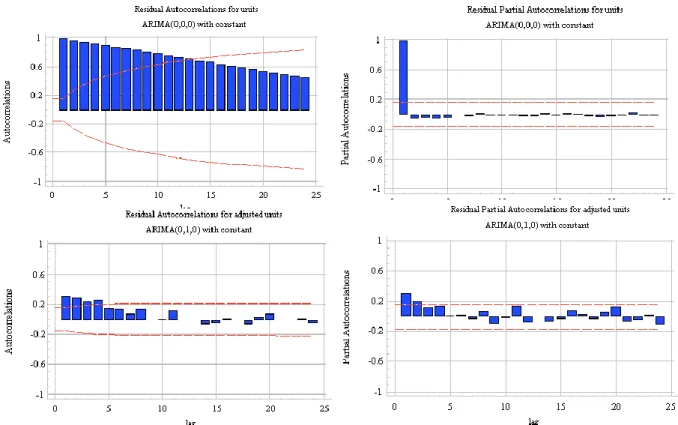
16 Below figure (Figure 5) represents a set of ACF and PACF plots for a sample series of data. The description of each scenario, as well as, possible interpretations of autoregressive and moving average terms has been presented below.

Figure 5: Examples of ACF and PACF plots and interpretations. (Robert Nau, 2019)

The visualization in the top left panel is an autocorrelation plot of the raw data. The autocorrelations look highly significant up to the 13th lag, which may be caused by the previously described propagation of autocorrelation at lag 1 (chaining effect). That is why, the top right panel of the Figure 5 represents a partial autocorrelation plot of the same series. Looking at the PACF plot, it is clear that lag-1 autocorrelation explains all remaining autocorrelations at the higher lags which are below the red line of significance level. This being said, it is safe to conclude that AR(1) model would be appropriate for the above series. Another possible approach to modelling above series is to perform a 1st order of non-seasonal differencing as a pre-processing step. The ACF and PACF plot of differenced data has been plotted in the bottom left and right panel of the Figure 5, respectively. Comparing the two graphs, it is clear that autocorrelations decay slower in the ACF plot, where all spikes up to 4 are significant, while in the PACF only the 2 initial spikes appear to be significant and then they shut off. This being said, the analysis of ACF and PACF plots on differenced data suggests modelling the series by means of the ARIMA(2,1,0) model, where 2 stands for the

(17)

17 autoregressive term, 1 indicated the order of differencing, and 0 means no moving average term used.

2.1.6. Types of Time Series Forecasting

Time series forecasting refers to predicting the future the most accurately as possible based on the information recorded at previous time steps. Based on the dimensionality of the analyzed data, Time Series Forecasting can be divided into two types:

- Univariate Modelling - Such forecasting methods use only the time and target value as inputs for modelling. An example of Univariate Modelling can be forecasting of the sales volume based on sales volumes recorded in the past.

- Multivariate Modelling – often a more efficient way of predicting a series of future values thanks to the advantage of using any additional information, such as knowledge of any future events which may impact the forecasts. Such models, where other than only time features are also used, can often make up for some fluctuations caused by some external factors, which could not be explained by regular trend, cycle or seasonal time components. An example of a multivariate modelling use-case can be a forecast of the air temperature based on not only air temperatures recorded in the past, but also, using the information about the rainfall, air humidity and the sunlight.

2.1.7. Forecast Error Metrics

The common goal of statistical predictions is to minimize the error of the predictions. The error can be defined as the difference between the forecast and its observed value. In time series, we should not understand the “error” as a mistake, but rather as a part of the observation, which is unpredictable. The formula for error calculation can be found below, where {y1, … ,yT} are the

train data, while {yT+1, yT+2,…} are the test data.

𝑒𝑇+ℎ = 𝑦𝑇+ℎ|𝑇− 𝑦̂𝑇+ℎ|𝑇 (3)

The errors differ from previously described residuals in two aspects. First of all, while residuals are calculated on the training set, the error is calculated on the validation set. Additionally, forecast errors can involve multi-step forecasts, which is not the case for residuals, as these are based on one-step forecast only.

There is a number of forecast error metrics which vary in different kinds of information used to identify the prediction accuracy. These can be classified into 3 categories:

(18)

18

- Scale-dependent errors

As the name suggests, scale-dependent errors cannot be used to compare between series involving different units, as they are scale dependent and expressed in some particular units. The most commonly used scale-dependent accuracy measures are based on absolute errors or squared errors, such as:

1. Mean Absolute Error (MAE) – an easily interpretable metric which treats errors in absolute terms, i.e. error of 10 is treated twice as bad as error of 5.

𝑀𝐴𝐸 = 1

𝑁∑|𝑍(𝑡) − 𝑍̂(𝑡)| 𝑁

𝑡=1

(4)

2. Root Mean Squared Error (RMSE) – gives a higher weight to large errors, penalizing them when they are very undesirable.

𝑅𝑀𝑆𝐸 = √1 𝑁∑ (𝑍(𝑡) − 𝑍̂(𝑡)) 𝑁 𝑡=1 2 (5) - Percentage errors

Percentage errors solve the problem of being scale-dependent, making a comparison of various time series possible, regardless of the units expressed in the time series. On the other hand, percentage errors’ downside is the fact that they are infinite or undefined if the true value that we are trying to predict equals zero. This being said, intermittent-demand data predictions should not be measured with the use of percentage errors due to zero demand values present in the series. Additionally, in case actual values oscillate around zero, the distribution of percentage errors can be very skewed.

The two most commonly used percentage errors involve:

1. Mean Absolute Percentage Error (MAPE) – an easily interpretable metric with a drawback of more heavy penalization on negative forecasting errors as compared to the positive forecasting errors.

𝑀𝐴𝑃𝐸 =1 𝑁∑ |𝑍(𝑡) − 𝑍̂(𝑡)| 𝑍(𝑡) 𝑁 𝑡=1 ∙ 100% (6)

(19)

19 2. Symmetric Mean Absolute Percentage Error (sMAPE) – a modified version of MAPE, created in the M3-competition (Makridakis & Hibon, 2000). The motivation behind this metric is to cancel the heavy penalization on negative forecasting errors, which is present in the classic MAPE metric. The downside of sMAPE is the fact that it does not eliminate the problem of division by a number close to zero, as a result it may lead to infinite error values for certain predictions. Finally, it is negative sMAPE values are possible making the interpretation ambiguous.

𝑆𝑀𝐴𝑃𝐸 = 1 𝑁∑ |𝑍(𝑡) − 𝑍̂(𝑡)| (𝑍(𝑡) + 𝑍̂(𝑡)) 𝑁 𝑡=1 ∙ 200 (7)

2.1.8. Cross-validation for Time Series

“It can not be emphasized enough that no claim whatsoever is being made in this paper that all algorithms are equivalent in practice in the real world. In particular no claim is being made that one should not use cross-validation in the real world.” - Wolpert (1994a)

It is important to appropriately estimate the accuracy of a model not only to predict the future prediction accuracy but also for choosing the best of the analyzed models (aka model selection) (Wolpert). The goal is to create a model yielding predictions with low bias and low variance. In order to correctly assess the results of statistical analysis or model-generated predictions, we need to ensure that our model will generalize to an independent data set. One way to achieve this is by applying validation methodology. The motivation to use cross-validation techniques is to verify how well the model will perform in practice, i.e. outside of a training set (in-sample data). Finally, cross-validation can also give us insights about potential underfitting (high bias, low variance) or overfitting (low bias, high variance) of the model.

(20)

20 The two most common validation techniques involve leave p out and K-fold cross-validation. The former randomly selects p samples as the validation set, using the rest of the samples as the training set. The latter creates random K equal-size partitions of the data, each of which is in turn used as a validation set, while the remaining K-1 subsets constitute for the training set. Unfortunately, there is a number of problems arising from applying these methods for Time Series Predictions:

- Autocorrelation along the time axis is a common component of a time series data. An example of such autocorrelation is car traffic, which affects all drivers on the route across consecutive time points. The randomization will most likely lead to presence of strong correlation of data samples from validation set and from the training set. Such phenomena breaks the purpose of validation set, which should be previously unseen by the model. In such case, the model virtually ‘knows’ about the validation set apriori, leading to the artificially good prediction accuracy, which is a sign of overfitting.

- Time series is a time-ordered series of data, in which past observations are used to predict the future. Standard cross-validation techniques involve randomization, which does not preserve the time ordering. A negative side-effect of traditional cross-validation for time series would be generating predictions for some samples using a model trained on posterior data points.

In the answer to above issues, a new cross-validation approach has been created for Time Series Predictions. One such methodology is known as Walk-Forward Cross Validation. This cross-validation technique involves arranging the data from past to present and splitting it to k equal blocks of contiguous samples, deciding that first p blocks will constitute a train set. This way, the training set consists of the blocks from 1 to p, while block p+1 is the validation set. After, the splits successively shift to the right, making the following split’s training set consist of blocks from 2 to p+1 and the validation set p+2, and so on. In this way, the ‘walking forward’ methodology leads to k-p splits. The visual representation of this methodology is presented at the Figure 7 below with the blue points representing training data and red points representing the validation data. For the final prediction accuracy, the chosen performance metric is averaged across the different folds. Of course, walk-forward cross validation allows to expand the validation period by more than one, i.e. it is possible to perform cross-validation

(21)

21 for weekly or monthly prediction (expanding the validation window by 7 or 30 data points, respectively and considering daily data).

Figure 7: Walk forward cross-validation technique with window size of one and four (Hyndman, R.J., & Athanasopoulos, G., 2018)

2.1.9. Data Preprocessing 2.1.9.1. Data Transformation

The main focus of time series data preprocessing lays in the data transformation methods. The most commonly used four data transformation methods for time series predictions include:

- Power Transform – makes the distribution more similar to Gaussian by removing a shift from data. In a time series dataset, it can be seen as a stabilization of variance over time. Some common examples of power transform methods include square root, cube root and log transformations.

- Difference Transform – this transformation is commonly used in order to make the mean, variance and covariance of a time series constant across time, i.e. in other words, stationary which is a prerequisite of some popular forecasting models (e.g. ARIMA). The 1st order differencing often helps to remove trend from a series of data, while kth differencing on a series with seasonality of length k should help remove the seasonal fluctuations. Difference transform methods are usually applied iteratively until the time series becomes stationary.

- Standardization – makes the distribution of the data similar to Gaussian. Standardization primarily consists of subtracting the mean and then dividing the result by a standard deviation of the data sample. As a result, transformed data has a mean of 0 and a standard deviation of 1, making it a standard Gaussian distribution.

(22)

22

- Normalization – a very common in Machine Learning transformation method leading to a scale adjustment within some boundaries (usually <0,1>). Such transformed time series is easier to be predicted by a forecasting model and often provides a better accuracy.

2.1.9.2. Missing Values Imputation

Missing values in a time series can be a result of a natural process, e.g. in the in-store sales time series there is no sales recorded on public holidays. Introducing a dummy variable indicating whether a given day is a public holiday is a possible way to approach such problem, avoiding the sales underestimation on the first day after the public holiday and then overestimations in the following days. However, in real-life dataset, the missing values are often not the result of a natural process but appear to be rather random. In such cases, the cause of missing values may be simply a device malfunction which did not record the data when needed or a human error in case the data is entered manually. In such scenarios, we can either take advantage of the models which work flawlessly even with missing data (e.g. Naïve Forecast) or make use of missing values imputation methods.

One way the null values in a time series may be imputed is by taking the series of data after the last missing value and generate a forecast of the next missing value, in effect replacing it with that prediction. Alternatively, it is possible to use simple computation methods like mean, median or mode imputation. In case of time series, however, there is also some special imputation methods, which include: Last Observation Carried Forward (LOCF), Next Observation Carried Backward (NOCB) and Linear Interpolation. The latter imputation methods rely on the assumption that adjacent observations are similar to each other, thus they do not work well when this assumption is not satisfied, especially in the presence of strong seasonality.

2.1.9.3. Outlier Imputation

Outliers are defined as observations that are very different from the majority of time series’ observations and can be seen on time series plots as sudden spikes or falls. As in the case of missing values, they can be simply erroneous data caused by e.g. a human error who entered the data manually or by a device malfunction. A common practice is to replace outliers with imputation methods described above in order to force the data to be more consistent with the majority of the series. One needs to be careful about replacing outliers without making sure that

(23)

23 these are in fact erroneous data, as they may often provide useful information about the underlying process which should be taken into consideration in the forecasting process.

2.2. TIME SERIES FORECASTING METHODS OVERVIEW

2.2.1. Evolution of time series analysis

In the nineteenth century early attempts to study time series were mostly based on the idea of a deterministic world until 1927, when the first major breakthrough in the area of time series forecasting took place essentially thanks to the contribution of Yule who introduced the notion of stochasticity in the time series. Simply put, Yule stated that every sequence of such data can be considered as the realization of a stochastic process, making this simple idea the base of further developed time series concepts over the years. More innovative forecasting concepts include the concept of autoregressive (AR) and moving average (MA) models formulated by Slutsky, Walker, Yaglom and Yule. Further, Kolmogorov (1941) proposed a solution to the linear forecasting problem relying on the idea of Wold’s decomposition theorem. After that, a vast research about time series parameter estimation, identification, model diagnosis and forecasting has been developed until a crucial revelation in the area of time series development was included in the publication by Box & Jenkins (1970, 1976) which was a vital integration of so-far existing knowledge. The book, making an enormous impact on the theory and practice of modern time series analysis and forecasting is also known for introducing a concept of Box-Jenkins approach, which is essentially a coherent, versatile three-stage iterative cycle for time series identification, estimation and verification. Investigation of time series forecasting methodology is remaining active until today with new approaches and extensions are being tested.

2.2.2. Time series forecasting methods

Time series forecasting falls onto a category of quantitative forecasting methods and serves a purpose to predict the manner in which the sequence of observations will continue into the future, using the series of past data collected at regular intervals of time (hourly, daily, weekly etc.).

Since there is a number of time series forecasting methods and none can be objectively indicated as better than other, an appropriate model selection needs to be made. Before deciding on the model type to be used, one needs to take into consideration both, time and computation resources, the data available, the accuracy of the competing models, as well as, the manner in which the forecasting model will be used. It is important to notice that time series forecasting

(24)

24 methods vary significantly in complexity. Some time series forecasting methods are as simple as a Naïve Forecast, which simply put, sets the all forecasts to be equal to the value of proceeding observation. This method is appropriate for data, which follows a random walk, such as economic or financial time series data, and is also known as a Random Walk Forecast.

𝑦̂𝑇+ℎ|𝑇 = 𝑦𝑇 (8)

Naïve Forecast can also be applied to a seasonal time series, where the forecast values are set as the last observed value of the same season of the year (e.g. the same day of previous week).

𝑦̂𝑇+ℎ|𝑇 = 𝑦𝑇+ℎ−𝑚(𝑘+1) (9)

Finally, another variation of the simplest forecasting methods has been created and named as Drift Method. Drift forecast model allows the forecasts to fluctuate up and down over time and sets the drift (i.e. change over time) to the average change recorded in the historical data. These models do capture the trend component but fail to do so with the seasonal component.

𝑦̂𝑇+ℎ|𝑇= 𝑦𝑇 + ℎ 𝑇 − 1∑(𝑦𝑡− 𝑦𝑡−1) 𝑇 𝑡=2 = 𝑦𝑇+ ℎ ( 𝑦𝑇− 𝑦1 𝑇 − 1 ) (10)

In addition to the above extremely simple and surprisingly effective time series forecasting methods, more advanced and widely used nowadays methods will be described and studied in the sections below.

2.2.3. Autoregressive Models

Similarly to multiple linear regression, where variable of interest is forecasted with use of a linear combination of predictors, the autoregressive models (AR) uses a linear combination of past values of target variable in order to predict the next values in the series. Thus, the autoregression term indicating that it is a regression of the target variable against itself. This model is suitable for a time series not exhibiting any trend nor seasonal components (stationary time series). An autoregressive model of order p AR(p) can be written as:

𝑍̃𝑡 = 𝜙1𝑍̃𝑡−1+ 𝜙2𝑍̃𝑡−2+ ⋯ + 𝜙𝑝𝑍̃𝑡−𝑝+ 𝑎𝑡 (11)

, where at represents white noise, putting an assumption that any element in a time series can

be represented as a random draw from a population distribution with constant variance and mean centered at 0.

(25)

25 Another possible notation for the AR(p) is following:

𝜙(𝐵)𝑍̃𝑡 = 𝑎𝑡 (12)

with a backshift operator defined as:

𝜙(𝐵) = 1 − 𝜙1𝐵 − 𝜙2𝐵2− ⋯ − 𝜙𝑝𝐵𝑝 (13)

The effect of backshift (aka Lag) operator is shifting the data back by one period. One single application of a backshift operator results in one backward shift of the data, while two such applications lead to shifting the data twice. In case the underlying process units are months and we wish to look at the data “same month last year”, then the appropriate notation looks as following B12yt=yt-12. Backshift operator is very useful when expressing the order of

differencing applied in the time series data preprocessing phase.

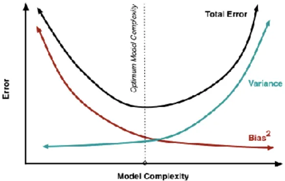
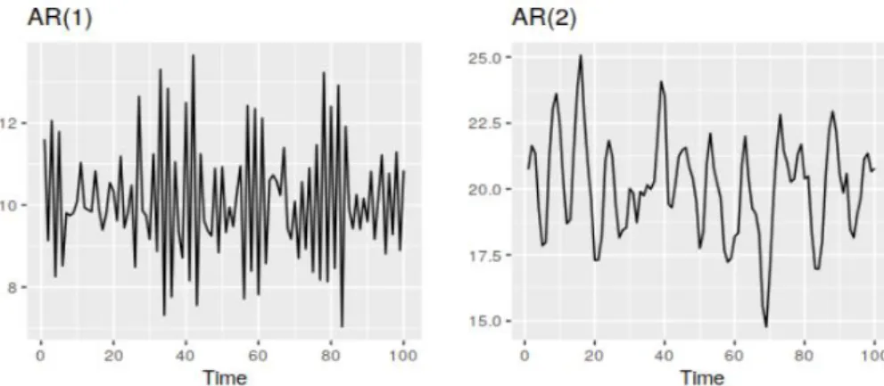
Finally, the variance of a white noise process is estimated from the data. There is no one best method to determine the correct order of autoregressive term for underlying process. Obtaining the right model should be the effect of trial and error supported with the guidance of Autocorrelation and Partial Autocorrelation Plots analysis. Optionally, one can use built-in functions provided by many data analysis softwares, such as auto.arima in pmdarima Python package, which conduct a search of all possible models, returning the one with the highest accuracy according to AIC, AICc or BIC criteria. It is worth noticing that models returned by such built-in functions will not always result in the highest possible accuracy, as criteria used in the search penalize for a number of parameters in the model for a lower model complexity. Below figure (Figure 8) illustrates two examples of Autoregressive Models.

Figure 8: Examples of data from autoregressive models with different parameters. (Hyndman, R.J., & Athanasopoulos, G., 2018)

(26)

26

2.2.4. Moving Average Models

Moving Average Models differ from Autoregressive Models in a way that a target value is forecasted with a regression-like model using past errors in place of the past values. Similarly to the autoregressive model, it is suitable for a time series not exhibiting trend nor seasonal components (stationary time series). Moving average model (MA) of order q can be written as:

𝑍̃𝑡 = 𝑎𝑡− 𝜃1𝑎𝑡−1− 𝜃2𝑎𝑡−2− ⋯ − 𝜃𝑞𝑎𝑡−𝑞 (14)

, where at represents white noise. Each value of yt can be defined as a weighted moving average

error of the past few forecast errors. One should be careful not to confuse one of well-known time series decomposition methods, i.e. moving average smoothing with the moving average model, as they serve different purposes. While moving average smoothing is used to estimate the trend and cycle of past values, a moving average model is used for forecasting future values of a series. Alternative notation for a moving average MA(q) model is following:

𝜃(𝐵) = 1 − 𝜃1𝐵 − 𝜃2𝐵2− ⋯ − 𝜃𝑞𝐵𝑞 (15)

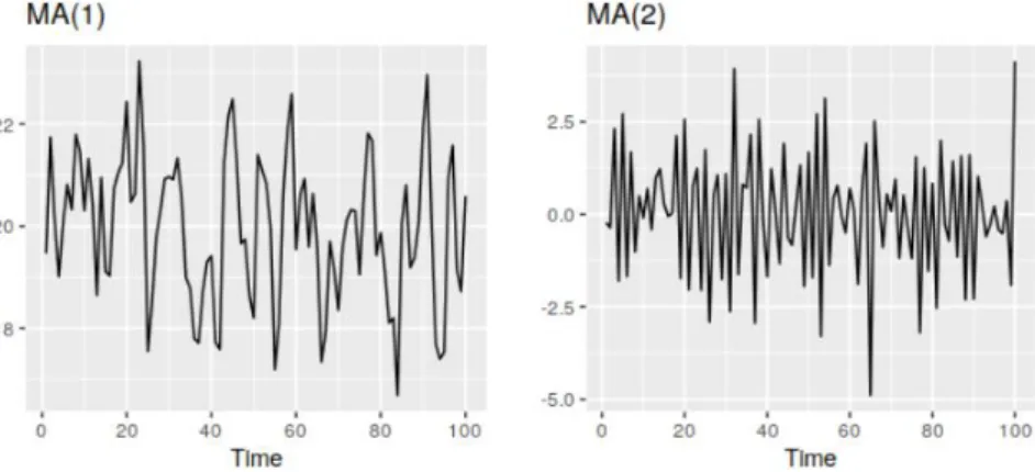
Similarly to the autoregressive models, the variance of white noise, as well as, the order of moving average term needs to be estimated from the data with analysis of Autocorrelation and Partial Autocorrelation plots, as well as, built-in statistical packages functions performing an automatic search for the best suited model. Below figure (Figure 9) illustrates two examples of Moving Average Models.

Figure 9: Examples of data from autoregressive models with different parameters(Hyndman, R.J., & Athanasopoulos, G., 2018)

2.2.5. ARIMA Models

Box and Jenkins proved in their publication of Time Series Analysis: Forecasting and Control (1970, 1976) that better prediction quality can be achieved by combining the autoregressive

(27)

27 with moving average models. In other words, ARIMA model uses a linear combination of the target variable’s past values, as well as, past forecasting errors for a new value prediction. A common notation for such a combined model is ARMA(p,q), which consists of an autoregressive component of order p, as well as, moving average component of order q. Additionally, in case the difference transform method was applied in the data preprocessing phase in order to remove the non-stationarity, then such model is referred as ARIMA(p,d,q), d parameter expressing the degree of first differencing. ARIMA(p,d,q) can be written as following:

𝑦𝑡′= 𝑐 + 𝜙1𝑦𝑡−1′ + ⋯ + 𝜙𝑝𝑦𝑡−𝑝′ + 𝜃1ℇ𝑡−1+ ⋯ + 𝜃𝑞ℇ𝑡−𝑞+ ℇ𝑡 (16)

, where y’t is a differenced time series.

Backshift notation of an ARIMA(p,d,q) model is presented below:

(1 − 𝜙1𝐵 − ⋯ − 𝜙𝑝𝐵𝑝)(1 − 𝐵)𝑑𝑦𝑡 = 𝑐 + (1 + 𝜃1𝐵 + ⋯ + 𝜃𝑞𝐵𝑞)𝜀𝑡 (17)

Last but not least, ARIMA works on the assumption of time series stationarity, thus should not be used unless this assumption is met. As in autoregressive and moving average models, appropriate values of p, d and q parameters need to be estimated by analyzing the autocorrelation and partial autocorrelation plots.

2.2.6. ARIMAX Models

Some processes can be best predicted when alongside the autoregressive and moving average terms, other exogenous variables are also used. ARIMAX is a modified version of the simple ARIMA, which is extended with a series of exogenous regressors with its coefficients. ARIMAX belongs to a family of multivariate models which tend to improve predictive accuracy by taking advantage of the information hidden in the valuable exogenous features. For instance, the air temperature may be predicted with use of solely time series, including autoregressive and moving average terms, however, the air temperature is also dependent on a series of other features, such as the rainfall or air humidity. Thus, this is a good example, where a series of temperature and rainfall records could be used as additional indicators to boost the model’s accuracy at predicting the air temperature at future time steps. Backshift notation of ARIMAX model is presented below:

(28)

28

2.2.7. SARIMA Models

SARIMA is a special kind of ARIMA model which involves additional seasonal AR and/or MA terms necessary to capture the patterns in a wide range of seasonal data. For instance, in case of monthly time series, it is often the case to see some annual patterns that repeat every 12 months, such as, December every year is a peak shopping season. In such series, it is advisable to consider using the seasonal first order autoregressive model, which would take advantage of data at time step xt-12 (December a year ago) to predict xt (next December). Apart from the

seasonal AR terms, SARIMA can also include seasonal MA terms, which take advantage of errors at time with lags which are multiples of S (span of seasonality).

For ARIMA modelling of a stationary series with a seasonal component, the model notation takes a form of SARIMA(p,d,q)(P,D,Q)_m, where p, d, q stand for the same aspects as in case of a non-seasonal ARIMA model, i.e. non-seasonal AR terms, differencing order, MA terms. Seasonal component is then described with the use of the P, D, Q parameters determining the seasonal autoregressive term, seasonal differencing order and seasonal moving average term, respectively. Finally, m stands for the number of time steps for a single seasonal period.

Backshift notation of an SARIMA(1,1,1)(1,1,1)12 is presented below:

(1 − 𝜙1𝐵)(1 − 𝝓1𝐵12)(1 − 𝐵)(1 − 𝐵12)𝑦𝑡 = (1 + 𝜃1𝐵)(1 + 𝜽1𝐵12) (19) 2.2.8. ARFIMA Models

Yet another type of ARIMA model is used in the presence of long memory in the series. In such cases, the Autoregressive Fractionally Integrated Moving Average (ARFIMA) model is used. This model is essentially a generalization of ARIMA thanks to the possibility of setting the differencing parameter as non-integer. The ARFIMA (p,d,q) belongs to a class of long memory models and its main objective is to account for the long term correlations in the data. Long memory can be identified by analyzing the autocorrelation plot (ACF) and is detected when deviations from the long-run mean decay more slowly as compared to the exponential decay. In essence, autocorrelation function in long memory models decays hyperbolically, as opposed to the “short term” ARIMA models exhibiting a geometric decay.

(29)

29

𝜙𝐵(1 − 𝐵)𝑑(𝑦_𝑡− 𝜇) = 𝜃(𝐵)𝜀𝑡, 𝜀𝑡~𝑖. 𝑖. 𝑑. (0, 𝜎𝜖

2₎ ₍₂₀₎

, where (1 − B)d_{is a fractional differencing operator.} 2.2.9. Artificial Neural Networks

Classical time series forecasting models suffer from a few limitations, which can be handled by applying more complex yet often more effective methods, such as artificial neural networks. The main limitations of classical time series forecasting methods that can be handled by ANNs include:

- Classical time series models are not suitable for forecasting a series following non-linear pattern

- Classical time series forecasting methods can usually work on univariate data only with the exception of (S)ARIMA methods which can be extended to multivariate forecasting ((S)ARIMAX)

- Lack of support for missing values

Deep Learning can be thought of as the most powerful area of machine learning with a constantly growing interest among various industries. Deep learning solutions can be applied to a wide range of problems from classical regression and classification problems to pattern recognition and time series forecasting. The power of artificial neural networks lays in the fact that they are capable of solving non-linear problems thanks to the non-linear function(s) applied to the inputs as they are propagated across the consecutive network layers. Additionally, ANNs don’t require feature selection as they perform it by themselves, setting weight values of particular neurons to nearly zero. Finally, they can solve a big variety of arbitrarily complex problems, searching for patterns in anything that can be translated into numbers, thus in pictures, sounds, and finally a series of data.

Of course, as any other method, neural networks also suffer from some drawbacks, such as a need for a big amount of data to train, long training time, as well as, it is considered a bit as a “black box”, i.e. it is relatively hard to comprehend the highly complex processes happening inside of a deep neural network. Finally, fine-tuning deep neural networks is extremely time consuming as the training consumes a lot of time and there is a wide range of parameters to tune (optimizer, activation function, number of layers, number of hidden neurons, and more…). Last but not least, the data used in a training process of a neural network needs to be of a much larger volume as compared to the standard machine learning models training. This is caused by the fact that deep neural networks have a relatively larger complexity and a bigger

(30)

30 number of parameters to optimize, in result requiring a larger amount of training examples before it can learn the underlying patterns. Finally, a good point of reference for guidelines on deep neural networks architecture setup can be found in the extensive summary available in Zhang et al. (1998).

2.2.10. Recurrent Neural Networks

Recurrent neural networks are a special kind of neural networks, which are designed to work on supervised learning problems with the data of sequential nature. Some examples of such problems which can be solved by RNN are speech recognition, video processing or time series forecasting.

Recurrent neural networks are in fact neural networks with memory, i.e. they are capable of remembering things from the past, which is essential when dealing with time-dependent problems. To produce accurate time series forecasts, RNNs use not only the input data but also the previous forecast values. Since simple passing values forward in time is not efficient enough, recurrent neural networks make use of some memory mechanism which helps the algorithm to filter to only the useful bits of data stored in memory and pass them to make a new prediction. The mechanism of memory in a recurrent neural network is used in order to imitate how the human brain works, i.e. the forecast of the next value in the sequence of data is not made from scratch every time a new information is passed into a model, however, a set of values which were previously passed is remembered, adding some extra context to the currently transferred piece of information. A recurrent neural network is an advancement of a traditional neural network, making it possible to model sequence data not only thanks to the memory unit providing context to the information inputs, but also giving a flexibility in terms of the inputs and outputs dimensions, i.e. RNNs are able to capture sequence-to-sequence relations with inputs and outputs in the form of sequences of vectors. Thanks to this capability, RNNs can easily provide a series of predictions of any length, being fed with multivariate, sequential inputs, which in turn can feed into the algorithm additional information in the form of exogenous variables (aka multivariate modelling). Additionally, recurrent neural networks have cyclical connections over time. During RNN training, an internal, maintained throughout the network state is constantly updated with activation functions, in turn providing a memory to the network. RNNs consist of a cycle besides the general information propagation existing in a traditional NN and thanks to this cycle information is not lost but passed forward across training steps.

(31)

31 The functioning of Recurrent Neural Network has been presented in the figure (Figure

10) below.

Figure 10: Recurrent Neural Network Loop (Christopher, 2015)

A traditional recurrent neural network can also be thought of as a list of copies of the same network, each of which is passing a message to a successor. Or, it can be also considered as a fully connected neural network if we spread out or unroll the time axis. (Kondratenko et al, 2003). In such way, each step of the RNN takes X as an input and returns h as an output, at the same time passing some information to the successor. It is crucial to mention that returned by each RNN’s component output’s content is not only impacted by the just-fed in input X but also by the whole history of inputs previously fed onto a network. The chain-like architecture of RNNs makes them a natural choice for lists and sequences of data, such as time series.

Even though traditional RNNs have been very successful in a wide range of applications requiring sequential data, the downside of classical RNNs is that they are not so good at handling long-term dependencies. For example, given a simple RNN a sequence of words “The clouds are in the…”, it does not require a broader context and is pretty obvious based on only recently passed information that predicted value of the sequence will be a word sky. However, in case the input sentences are longer, such as “I grew up in Germany (…). I speak fluent…”, the RNN indeed needs a broader context and needs to look further in the past to find out that predicted word should be German. This is an example of a challenge which a classical RNN will most likely fail to solve, as the gap between relevant information and currently predicted value is too large. Indeed, RNNs become unable to learn to connect relevant information as that gap grows. Theoretically speaking, RNNs should have the capability to capture such long-term dependencies, however, Hochreiter (1991) and Bengio, et al. (1994) proved that this is not the case. This problem is known as a vanishing gradients problem and occurs when long sequences of data need to be learnt. The core of vanishing gradients problem lays in the fact that the longer

(32)

32 the data sequence is, the further the gradients need to carry the information used in the RNN parameter update, making these updates become extremely small, in effect not learning at all. According to (Xavier et al 2011) ReLU activation function slows down the vanishing gradient problem, as compared to the sigmoid function.

2.2.11. Long Short-Term Memory Network

Long Short Term Memory networks are a special kind of recurrent neural networks, which can deal better with the gradient vanishing problem, making LSTMs capable of learning long-term dependencies. Hochreiter & Schmidhuber (1997) were the ones to introduce and popularize this algorithm. LSTMs are known for their outstanding accuracy, when its parameters are carefully set-up. Additionally, remembering long-term dependencies is something that they are cut out for.

The structure of this powerful algorithm has been presented below:

Figure 11: LSTM Memory Cell (Christopher, 2015)

LSTMs, just like standard RNNs, are in the form of a chain of repeating modules. What differs them however, is the structure of these modules, as instead of having a single neural network layer in each as classical RNNs do, they consist of four layers interacting with each other in a precise way. The horizontal line running across above part of the diagram presents the core idea behind LSTM and is known as the cell state. The main role of the cell state is to propagate the information, leaving it unchanged, adding relevant and removing irrelevant pieces of information which is structured by the gates. The forget gates are composed of a sigmoid layer and a point-wise multiplication operation. The output of the sigmoid layer is a value between zero and one, determining how much information should be let through (and forgotten) into the cell state. The next step is the input gate, which is essentially a hidden layer of sigmoid activated nodes, outputting values between 0 and 1 that are able to control the amount of input which will flow into the unit. The tanh layer creates a vector of new candidate values which can be added

(33)

33 to the state. Finally, the output gate determines with the use of a sigmoid function which values of the state will serve as the output from the cell.

The flexibility of LSTM is provided thanks the number of gating functions controlling what needs to be forgotten and remembered by the network. However, as Machine Learning is known to be a science of trade-offs, here is no exception made, and thus the flexibility of LSTM also comes with the cost of a big number of parameters that need to be fine-tuned for the network to perform efficiently, making it computationally expensive to train.

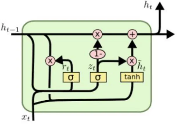
2.2.12. Gated Recurrent Units

A gated recurrent unit has been introduced by Cho, et al. (2014) as a newer generation of RNNs. It works similarly to LSTMs with two main differences: instead of a cell state, GRU uses a hidden state in order to propagate the information. Additionally, GRU has only two gates: a reset and update gate. Gated recurrent unit has been introduced as an alternative to LSTMs, which would be still able to avoid the vanishing gradient problem, but would not have such a big number of parameters to tune and would be less computationally complex. In addition, according to the research of Tang, et al. (2017), GRU is more robust to noise as compared to LSTM and it tends to outperform LSTM in several applications.

The GRU unit architecture has been presented in the diagram below:

Figure 12: Gated Recurrent Unit Cell (Christopher, 2015)

The update gate in a GRU unit serves a similar purpose as the forget and input gates of an LSTM, i.e. it controls the amount of past information that needs to be passed to the next step, as well as, what new information to add. The reset gate on the other hand is used to determine the amount of past information to forget. Due to the fact that GRU unit consists of only two gates, it is faster to train as compared to LSTM.

(34)

34

3. RELATED WORK

3.1. POSSIBLE TIME SERIES APPLICATIONS

The analysis of experimental data recorded at different points in time requires a special approach as it leads to new and unique problems in the field of statistical modelling and inference. This is mainly due to the nature of time series breaks the assumption of many conventional statistical methods, which rely on the fact that the observations are independent and identically distributed. The below-described list of fields where time series problems may arise is a proof of the impact that time series analysis may have on diverse scientific applications. One of the most common time series applications can be found in the field of economics, where daily stock market quotations or monthly employment rates need to be analyzed and predicted. Other examples of time series analyses’ applications include socio-demographic series, such as school enrollments, birth rates, gender or fertility tendencies. In medicine, on the other hand, analysis of blood pressure measurements over time might be useful for evaluating drugs used in treating hypertension. Time series in combination with computer vision in the form of a series of magnetic resonance imaging can be effective for analysis of the brain’s reaction to certain stimuli under various experimental conditions. Finally, a number of sophisticated applications of time series methodologies have been practiced in the environmental and physical sciences. This being said, the monthly sunspot numbers are one of the earliest recorded series studied by Schuster (1906). Environmental sciences rely on time series also in more modern investigations, such as global temperature measurements and analysis of global warming evolution. Speech series modelling is another important area where time series analysis is used and it makes the transmission of voice recordings efficient. Rainfall and air temperature may also be predicted based on geophysical time series. Finally, seismic recordings over time can be useful to differentiate the earthquakes from nuclear explosions. Above listed examples of time series analysis applications are just a few of all that are being used nowadays.

3.2. TIME SERIES COMPARATIVE STUDIES

There is a number of studies focusing on comparison of traditional time series analysis methodology with the methods from the family of Artificial Neural Networks. With the use of a dataset from the famous “M-3 competition” Foster, et.al. (1991) proved that deep neural networks are inferior to the least squares statistical models for a yearly tie series data. The results of studies conducted by Sharda and Patil (1992) and Tang, et.al. (1991) argued that for

(35)

35 a large number of observations, ANN models and Box-Jenkins models deliver similarly good results. Kang (1991) observed in his study comparing 18 different neural network architectures that forecast errors tend to be smaller for the series which contain the trend and seasonal component. Additionally, according to Kang the neural networks often outperform the simple statistical time series forecasting models in the long horizon forecast periods. Another study comparing neural networks to the traditional forecasting methods have been performed by Hill, et.al. (1996) who compared his forecasts to those obtained by Makridakis, et.al. (1982) and concluded that ANNs do better for monthly and quarterly series. Another conclusion driven by their study is that fewer network parameters to be estimated is crucial to successful neural network modelling. Kohzadi, et.al. (1996) is the owner of a very controversial statement, that he has made based on his empirical investigation aiming at comparing the forecasting performance of ANNs to ARIMA model: “The neural network with only one hidden layer can precisely and satifactorily approximate any continuous function” (Kohzadi, et.al., 1996, p.179). Kohzadi, et.al. (1996) has also concluded that ANNs are more efficient at catching the turning points of the series when compared to ARIMA model. However, some of the studies conducted by Adya and Collopy (1998) based on 48 articles published between 1988 and 1994 resulted in contradicting to Kohzadi’s statements, indicating that real-world data may not always be consistent with theoretical inferences.

Even though a big part of the time series literature is focused on modelling time series data and comparing the performance of various competing models, Gorr, et.al. (1994) used cross section data to predict the values of student grade point averages and compared the predictive power of a linear regression and a stepwise polynomial regression versus the ANN. Based on these studies, they have concluded that the mean errors of forecasts generated by different models were not comparable as none of the models was significantly superior compared to the others. This result has been justified by the selection ANN structure. However, it can be also argued that another reason for the unsatisfactory results delivered by the neural network is the fact that qualitative binary variables have been used in 6 of the models. In such cases, ANN learning algorithm may not work well due to the large numerical distinction in the observations between the binary and continuous variables.

The effect of a time series stationarity on the forecasting performance of the statistical and deep learning models has been tested by Lachtermacher and Fuller (1995) in their study of a series of annual river flows. Lachtermacher and Fuller followed Box-Jenkins methodology to produce an ARIMA model, as well as, the ANN model. They have concluded that the ANN