Universidade de Aveiro 2014
Departamento de Eletrónica, Telecomunicações e Informática
Luis Miguel Lima de
Almeida
Processamento ótico baseado em ótica integrada
Universidade de Aveiro 2014
Departamento de Eletrónica, Telecomunicações e Informática
Luis Miguel Lima de
Almeida
Processamento ótico baseado em ótica integrada
All-optical processing based on integrated optics
Dissertação apresentada à Universidade de Aveiro para cumprimento dos requisitos necessários à obtenção do grau de Mestre em Engenharia Eletrónica e Telecomunicações, realizada sob a orientação científica do Dr. António Teixeira, Professor do Departamento de Eletrónica, Telecomunicações e Informática da Universidade de Aveiro
Dissertation submitted to the University of Aveiro in the fulfilment of the requirements for the degree of Master in Electronics and Telecommunications Engineering, under the supervision of Doctor António Teixeira, Professor in the Department of Electronics, Telecommunications and Informatics of the
University of Aveiro.
Apoio financeiro do projecto CITO PTDC/EEA-TEL/114838/2009.
Dedico este trabalho à minha família pelo apoio prestado em toda a formação académica.
o júri / the jury
Presidente / president Professor Doutor Armando Humberto Moreira Nolasco Pinto
Professor associado da Universidade de Aveiro
Vogais / examiners commitee Professor Doutor António Luís Jesus Teixeira
Professor associado com agregação da Universidade de Aveiro (orientador)
Doutor Carlos Miguel Santos Vicente
Agradecimentos/ Acknowledgements
I wish to thank to my supervisor Doctor António Teixeira for his orientation, guidance and encouragement during this work. I would also like to thank to Dr. Giorgia Parca, Dr. Naresh Kumar, Ana Lopes and professor Uwe Kahler for the help, advice and guidance during this work. It was a pleasure to work with all of them.
I wish to express a special gratitude for the financial support given by the CITO project PTDC/EEA-TEL/114838/2009 and to the Telecommunications Institute for all the support provided.
Last, but not least, my warm thanks to my family, girlfriend and friends for their love, help and understanding throughout my life. I would not have come so far without them.
palavras-chave Ótica integrada, transformada de onduletas, transformada de onduletas de Haar, compressão de imagem, acoplador, Waveshaper, Matlab.
resumo Nos últimos anos, a procura por elevados ritmos de transferência de
informação em comunicações óticas tem aumentado exponencialmente. Dado que imagem, no seu formato original exactamente como é captada pela câmara fotográfica ocupa enormes quantidades de espaço de
armazenamento, torna-se importante desenvolver um sistema que aumente o seu grau de compressão, preservando as informações importantes da imagem. No tópico da compressão de imagem existem várias técnicas de
transformação usadas para compressão de dados. A transformada discreta de onduleta é uma das mais usadas, graças ao uso da transformação em multi-resolução. Esta propriedade de multi-resolução permite não só desenvolver métodos de compressão de imagem sem perdas, nos quais se obtém a imagem original exatamente como era antes da transformação, como também métodos com perdas, já não sendo possível obter a imagem original.
Neste contexto, esta tese irá desenvolver a ideia de aplicar a transformada de onduleta de Haar usando circuitos óticos. Este conceito irá ser analisado, verificando a possibilidade da sua implementação no domínio ótico, usando vários métodos, com perdas e sem perdas, para concluir acerca do melhor método de compressão a aplicar a uma imagem. Por fim, o método com perdas irá ser testado no laboratório com diferentes componentes e desenhar o dispositivo ótico capaz de aplicar a transformada de onduleta de Haar.
keywords Integrated optics, wavelet transforms, Haar wavelet transform, image compression, coupler, Waveshaper, Matlab.
abstract During the last years, the demand for high data transfer rates in optical fiber
communications has increased exponentially. Since image in its original format exactly as it is captured by the digital camera requires an enormous amount of storage capacity, it is important to develop a system that increases its amount of compression while preserving the important image’s information.
In the topic of image’s compression, there are several transformation
techniques used for data compression. Discrete Wavelet Transform (DWT) is one of the most commonly used, thanks to its multi-resolution transformation. This multi-resolution property allows to develop, not only a lossless
compression method, from which the original image can be obtained exactly as it was before the transform, but also, a lossy method where it is not possible to obtain the original image.
In this context, this thesis will develop the idea to apply the Haar wavelet transform using optical circuits. This concept will be analyzed, verifying the possibility of its implementation in the optical domain, using several methods, lossy and lossless, to conclude about the best compression method to apply to an image. Finally, the lossy method will be tested in the laboratory with different components and design the optical device able to accomplish the Haar wavelet transform.
Contents
Contents i
List of Figures iii
List of Tables ix Acronyms xi Chapter 1: Introduction 1 1.1MOTIVATION ... 2 1.2OBJECTIVES ... 2 1.3THESIS ORGANIZATION ... 3 1.4MAIN ACHIEVEMENTS ... 4
Chapter 2: Image compression 7
2.1IMAGE COMPRESSION TRANSFORMATIONS METHODS ... 7
2.2LOSSY VS LOSSLESS ... 7
2.3IMAGE FORMATS ... 8
2.4DISCRETE WAVELET TRANSFORM ... 9
2.4.1 Haar transform – based image compression system... 10
2.4.2 Optical Haar transform device ... 12
2.5IMAGE QUALITY ASSESSMENT PARAMETERS ... 15
Chapter 3: Theoretical implementation of the optical system in Matlab ... 19
3.1IMPLEMENTATION OF THE HAAR WAVELET TRANSFORM ... 19
3.1.1 Lossless compression ... 21
3.1.2 Lossy compression ... 22
3.1.2.1 Lossy compression with variation in the amplitude of the parameters of the Haar transformation matrix ... 24
3.1.2.2 Lossy compression with variation in the phase of the parameters of the Haar transformation matrix ... 27
3.2IMPLEMENTATION OF ADDITIONAL COMPRESSION IN THE DATA ENCODING PROCESS ... 30
3.2.1 Additional compression with threshold ... 30
3.2.2 Additional compression with quantization ... 32
Chapter 4: Laboratory experiment with the Haar wavelet transform ... 35
4.1VISIBLE SPECTRAL REGION (635 NM WAVELENGTH) ... 35
4.1.1 Setup ... 35
4.1.2 Results ... 37
4.1.3 Image comparison ... 39
4.1.3.1 4x4 Image with moderate contrast: ... 39
4.2.3.2 4x4 Image with high contrast: ... 40
4.1.4 Discussion of results... 41
4.2C BAND (1550 NM WAVELENGTH) ... 41
4.2.1 Setup ... 42
4.2.2 Results ... 45
4.2.3 Image comparison ... 47
4.2.3.2 4x4 Image with high contrast: ... 48
4.2.3.3 4x4 Image with low contrast: ... 49
4.2.3.4 8x8 Image with moderate contrast: ... 50
4.2.4 Discussion of results... 51
Chapter 5: Optical Haar transform design 53
5.1PHOENIXOPTODESIGNER ... 53
5.23DB ASYMMETRIC COUPLER DESIGN ... 53
5.3OPTICAL HAAR TRANSFORM DESIGN ... 56
5.4DISCUSSION OF RESULTS ... 58
Chapter 6: Conclusion and future work 63
References 65
List of Figures
Figure 1: Data growth by year [2]. ... 1
Figure 2: Process of a two level signal decomposition using multi-resolution analysis. ... 10
Figure 3: System building blocks for Haar optical wavelet transform (OWT) based on all-optical processing and compression. 2D transform process schematic describes low-pass (L) and high-pass (H) filtering until sub-band decomposition [16]. ... 11
Figure 4: 3 dB asymmetric optical coupler scheme and scattering matrix [16]. 13 Figure 5: 3D basic module for 1st-level optical 2D HT [16]. ... 13
Figure 6: Integrated passive scheme for Optical WT-IWT; passive compression is accomplished by spatial selection of the LL coefficients, delivered through reported connections [16]. ... 14
Figure 7: Haar wavelet transform applied to the image "TIF-1". ... 21
Figure 8: Size and image format comparison in lossless compression. ... 22
Figure 9: Size and image format comparison in lossy compression. ... 23
Figure 10: Compression ratio and file format of the image. Comparison by compression method. ... 24
Figure 11: MSE and amplitude variation in the Haar transform matrix comparison. ... 25
Figure 12: PNSR and amplitude variation in the Haar transform matrix comparison. ... 26
Figure 13: Quality and amplitude variation in the Haar transform matrix comparison. ... 27
Figure 14: MSE and phase variation in the Haar transform matrix comparison. ... 28
Figure 15: PNSR and phase variation in the Haar transform matrix comparison. ... 29
Figure 16: Quality and phase variation in the Haar transform matrix comparison. ... 29
Figure 17: Number of occurrences of each pixel (symbol) by level of threshold ... 31
Figure 18: Number of occurrences of each pixel (symbol) by level of quantization
... 33
Figure 19: Image 4x4 with moderate contrast. ... 35
Figure 20: Image 4x4 with high contrast. ... 35
Figure 21: Setup with a 3dB coupler. ... 37
Figure 22: Photography of the 635 nm setup. ... 37
Figure 23: Theoretical Scaling image. ... 39
Figure 24: Obtained Scaling image from scheme 1 with IL. ... 39
Figure 25: Obtained Scaling image from scheme 1 without IL. ... 39
Figure 26: Obtained Scaling image from scheme 2 with IL. ... 40
Figure 27: Obtained Scaling image from scheme 2 without IL. ... 40
Figure 28: Theoretical Scaling image. ... 40
Figure 29: Obtained Scaling image from scheme 3 with IL. ... 41
Figure 30: Obtained Scaling image from scheme 3 without IL. ... 41
Figure 31: Image 4x4 with moderate contrast [22]. ... 42
Figure 32: Image 4x4 with high contrast [22]. ... 42
Figure 33: Image 4x4 with low contrast [22]. ... 42
Figure 34: Image 8x8 with moderate contrast [22]. ... 42
Figure 35: Setup with 3dB coupler. ... 44
Figure 36: Photography of the 1550 nm setup with 3dB coupler. ... 44
Figure 37: Setup with Waveshaper. ... 44
Figure 38: Photography of the 1550 nm setup with Waveshaper. ... 45
Figure 39: Theoretical Scaling image [22]. ... 47
Figure 40: Obtained Scaling image from the 3dB coupler with IL. ... 47
Figure 41: Obtained Scaling image from the 3dB coupler without IL [22]. ... 47
Figure 42: Obtained Scaling image from the Waveshaper with IL. ... 48
Figure 43: Obtained Scaling image from the Waveshaper without IL. ... 48
Figure 44: Theoretical Scaling image [22]. ... 48
Figure 45: Obtained Scaling image from the 3dB coupler with IL. ... 48
Figure 46: Obtained Scaling image from the 3dB coupler without IL [22]. ... 48
Figure 47: Obtained Scaling image from the Waveshaper with IL. ... 49
Figure 48: Obtained Scaling image from the Waveshaper without IL. ... 49
Figure 49: Theoretical Scaling image [22]. ... 49
Figure 51: Obtained Scaling image from the 3dB coupler without IL [22]. ... 49
Figure 52: Obtained Scaling image from the Waveshaper with IL. ... 50
Figure 53: Obtained Scaling image from the Waveshaper without IL. ... 50
Figure 54: Theoretical Scaling image [22]. ... 50
Figure 55: Obtained Scaling image from the 3dB coupler with IL. ... 51
Figure 56: Obtained Scaling image from the 3dB coupler without IL [22]. ... 51
Figure 57: Obtained Scaling image from the Waveshaper with IL. ... 51
Figure 58: Obtained Scaling image from the Waveshaper without IL. ... 51
Figure 59: 3 dB asymmetric coupler geometry and design [22]. ... 54
Figure 60: Schematic of the optical Haar transform [22]. ... 57
Figure 61: Power propagation along the optical Haar transform schematic for Experiment 1 [22]. ... 60
Figure 62: Phase propagation along the optical Haar transform schematic for Experiment 1 [22]. ... 61
Figure 63: TIF 1 - Original image. ... 69
Figure 64: TIF 1 - Haar transform image. ... 69
Figure 65: TIF 1 - Scaling image of the Haar transform. ... 69
Figure 66: TIF 2 - Original image. ... 69
Figure 67: TIF 2 - Haar transform image. ... 69
Figure 68: TIF 2 - Scaling image of the Haar transform. ... 69
Figure 69: TIF 3 - Original image. ... 70
Figure 70: TIF 3 - Haar transform image. ... 70
Figure 71: TIF 3 - Scaling image of the Haar transform. ... 70
Figure 72: TIF 4 - Original image. ... 70
Figure 73: TIF 4 - Haar transform image. ... 70
Figure 74: TIF 4 - Scaling image of the Haar transform. ... 70
Figure 75: JPEG 1 - Original image. ... 71
Figure 76: JPEG 1 - Haar transform image. ... 71
Figure 77: JPEG 1 - Scaling image of the Haar transform. ... 71
Figure 78: JPEG 2 - Original image. ... 71
Figure 79: JPEG 2 - Haar transform image. ... 71
Figure 80: JPEG 2 - Scaling image of the Haar transform. ... 71
Figure 81: JPEG 3 - Original image. ... 72
Figure 83: JPEG 3 - Scaling image of the Haar transform. ... 72
Figure 84: JPEG 4 - Original image. ... 72
Figure 85: JPEG 4 - Haar transform image. ... 72
Figure 86: JPEG 4 - Scaling image of the Haar transform. ... 72
Figure 87: BMP 1 - Original image. ... 73
Figure 88: BMP 1 - Haar transform image. ... 73
Figure 89: BMP 1 - Scaling image of the Haar transform. ... 73
Figure 90: BMP 2 - Original image. ... 73
Figure 91: BMP 2 - Haar transform image. ... 73
Figure 92: BMP 2 - Scaling image of the Haar transform. ... 73
Figure 93: BMP 3 - Original image. ... 74
Figure 94: BMP 3 - Haar transform image. ... 74
Figure 95: BMP 3 - Scaling image of the Haar transform. ... 74
Figure 96: BMP 4 - Original image. ... 74
Figure 97: BMP 4 - Haar transform image. ... 74
Figure 98: BMP 4 - Scaling image of the Haar transform. ... 74
Figure 99: PNG 1 - Original image. ... 75
Figure 100: PNG 1 - Haar transform image. ... 75
Figure 101: PNG 1 - Scaling image of the Haar transform. ... 75
Figure 102: PNG 2 - Original image. ... 75
Figure 103: PNG 2 - Haar transform image. ... 75
Figure 104: PNG 2 - Scaling image of the Haar transform. ... 75
Figure 105: PNG 3 - Original image. ... 76
Figure 106: PNG 3 - Haar transform image. ... 76
Figure 107: PNG 3 - Scaling image of the Haar transform. ... 76
Figure 108: PNG 4 - Original image. ... 76
Figure 109: PNG 4 - Haar transform image. ... 76
Figure 110: PNG 4 - Scaling image of the Haar transform ... 76
Figure 111: Haar inverse transform from image TIF 1 after a threshold level of 0 ... 77
Figure 112: Haar inverse transform from image TIF 1 after a threshold level of 4 ... 77
Figure 113: Haar inverse transform from image TIF 1 after a threshold level of 8 ... 77
Figure 114: Haar inverse transform from image TIF 1 after a threshold level of 16 ... 77 Figure 115: Haar inverse transform from image TIF 1 after a threshold level of 32 ... 78 Figure 116: Haar inverse transform from image TIF 1 after a threshold level of 64 ... 78 Figure 117: Haar inverse transform from image TIF 1 after a threshold level of 128 ... 78 Figure 118: Haar inverse transform from image TIF 1 after a quantization level of 1 ... 78 Figure 119: Haar inverse transform from image TIF 1 after a quantization level of 2 ... 79 Figure 120: Haar inverse transform from image TIF 1 after a quantization level of 5 ... 79 Figure 121: Haar inverse transform from image TIF 1 after a quantization level of 10 ... 79 Figure 122: Haar inverse transform from image TIF 1 after a quantization level of 20 ... 79 Figure 123: Haar inverse transform from image TIF 1 after a quantization level of 50 ... 80
List of Tables
Table 1: Characteristics of the images used for comparison. ... 20 Table 2: Quality assessment parameters by level of threshold ... 32 Table 3: Quality assessment parameters by level of quantization ... 34 Table 4: Power range used with the 3dB coupler setup. ... 36 Table 5: Schemes comparison for the 635 nm wavelength. ... 38 Table 6: Power range used with the 3dB coupler setup. ... 43 Table 7: Power range used with the Waveshaper setup. ... 43 Table 8: Insertion loss and average Standard Deviation comparison. ... 45 Table 9: MSE and PSNR comparison. ... 46 Table 10: Parameters for the simulated 3dB asymmetric coupler. ... 56 Table 11: Output values from the simulated 3db asymmetric coupler [22]. ... 56 Table 12: Parameters for the optical Haar transform schematic. ... 58 Table 13: Input and theoretical output value in each port of the optical Haar transform. ... 59 Table 14: Theoretical and output value in each port of the optical Haar transform. ... 60
Acronyms
1D One-dimensional space 2D Bi-dimensional space A/m Amplitude per meter BMP Bitmap Image File (.bmp) Bpp Bits per pixel
CMT Coupled Mode Theory dB Decibels
dBm Decibel milliwatts
DCT Discrete Cosine Transform DFT Discrete Fourier Transform DWT Discrete Wavelet Transform ECL External Cavity Lasers IL Insertion Loss
JPEG Joint Photographic Experts Group (.jpg) kB Kilobyte
MSE Mean Square Error mW milliwatt
Nm Nanometers
OWT Optical Wavelet Transform
PNG Portable Network Graphics (.png) PSNR Peak Signal to Noise Ratio
RGB Red, Green, and Blue (primary colors) ROI Region of Interest
TE Transverse Electric mode
TIF Tagged Image File Format (.tiff) TLS Tunable Laser Source
WHT Walsh Hadamard Transform µm Micrometers
Chapter 1: Introduction
“The real voyage of discovery consists not in seeking new landscapes, but in having new eyes” Marcel Proust
It is said that a picture is worth a thousand words. However, in this modern internet age, the demand for data transmission and data storage is increasing. As seen in Figure 1, the data growth is about 40% every year, reaching nearly 45 Zettabytes by the year 2020. Study has shown that the 90% of total volume of data in internet access consists of image and video related data [1], making this field of study very important to reduce that amount of data. Image in their raw (uncompressed) format requires huge storage space. Such raw data needs large transmission bandwidth for the transmission over the network. Hence, many researchers have been conducted in the field of data compression system.
Figure 1: Data growth by year [2].
Compression techniques reduces the size of data, which in turn, requires less bandwidth, less transmission time and related cost. For that, they use compression algorithms, which assume that there is some bias on the input message of the data, so that some inputs are more likely than others. Most algorithms base this “bias” on the structure of the message, that there is some unbalanced probability distribution over the possible messages [3]. There are
algorithms developed for the data compression such as Discrete Cosine Transform (DCT), Discrete Wavelet Transform (DWT), Walsh Hadamard Transform (WHT), etc.
1.1 Motivation
Optical circuitry has recently become a very active research field due to the massive amount of real-time data via limited bandwidth channels. The advantage of optics is its capability of providing high count of parallel operations in a three dimensional space.
Some work has already been developed so far on the field of data processing using transforms. For example, on free-space optics using the Fourier transform as described in [4] or wavelet based models for propagation in optical fibers accordingly to [5]. In addition, the medical and security/encryption fields have shown a lot of interest in image compression due to the lack of secure and fast optical transmission channels, as presented in [6], [7] and [8].
Image compression suffers from large computational requirements. These types of data have to be compressed during the transmission process. Techniques that previously dominated the field such as Fourier transforms now have to compete with many other integral transforms and in particular with wavelet transforms. Wavelet analysis is a particular time or space scale representation of signals, which has found a wide range of applications in signal processing, physics and applied mathematics. 2D discrete wavelet transform (DWT) has been the most relevant, emerging image compression approach in such a way that it was adopted as the JPEG2000 standard [9].
1.2 Objectives
In this thesis, an all-optical processor based on integrated optics is presented. The two dimensional Discrete Wavelet Transform (DWT) will be applied on the data block of an image to implement a compression method. To begin with,
different compression methods will be studied: lossy compression, lossless compression, with threshold and with quantization. Then, a small part of the DWT image will be retrieved, the so called “Scaling image”, to study the possibility of a lossy compression method between optical devices in different wavelengths. If the compression method proves to be successful, the aim of the work will be deviated to the implementation of the complete DWT with the device Finisar Waveshaper 4000s, creating a lossless compression method.
The main objective of this thesis is to investigate the performance of the proposed all-optical processing based on integrated optics for wide range of image formats and applications.
1.3 Thesis organization
This thesis is organized in a clear and concise way for the reader to understand it in the simplest way possible:
Chapter 2: Image compression - For a better understanding of the following chapters, a brief explanation about image compression will be given in this chapter, starting with image compression transform methods. After that, a comparison between lossy and lossless compression will also be done, right after an explanation about Discrete Wavelet Transform, the image formats that will be used in this work and the most important subject of analysis. Related to it, the Haar wavelet transform and optical device will be explained. To finish with in this chapter, the image quality assessment parameters used will be defined.
Chapter 3: Theoretical implementation of the Haar wavelet transform - In this chapter, the Haar wavelet transform will be implemented and analyzed using the software Matlab, comparing different compression methods (lossy and lossless) and parameters variation in the Haar transform matrix. Two additional methods will also be studied, using the lossless compression method. An amount of threshold or quantization is applied to reduce the number of symbols in the image, increasing the data transmission speed.
Chapter 4: Laboratory experiment with the Haar wavelet transform - In this chapter, the Haar wavelet transform will be applied in the laboratory with two wavelengths, using real devices to check the practical use of the Haar transform when some errors are introduced. To begin with, a lossy compression method will be used. Then, if the lossy compression method proves to be successful, the focus will be moved to a lossless compression method using the component Finisar Waveshaper 4000s.
Chapter 5: Optical Haar transform design - In this chapter, an optical Haar transform will be designed and simulated using the software OptoDesigner. The refractive index of some materials used in the manufacturing of optical fiber circuits will be used, making it possible to build the device in the future.
Chapter 6: Conclusion and future work - In this chapter, the main conclusions of the previous chapters will be presented, as well as a perspective of the points that might be improved in the future, thus continuing the work developed so far.
1.4 Main achievements
With the work developed in this thesis, the following achievements were accomplished:
All-optical system based on the Haar Wavelet transform capable of obtaining significant compression ratio with low loss of quality in image files;
The setup with the 3dB coupler for the C band, has shown to provide images with high compression ratio and quality;
With the design of the optical Haar transform, an optical device that performs successfully a lossy compression method based on the Haar wavelet transform;
A publication in ICTON 2014:
Shahpari, “All-Optical Image Compression Processing Based on Integrated Optics”, 16th International Conference on Transparent Optical Networks, IEEE, 2014.
Chapter 2: Image compression
2.1 Image compression transformations methods
Image is digitally represented in a group of pixels. Usually the neighboring pixels are correlated to each other and are redundant in the image. The redundancy occupies unnecessarily storage space, which decreases the transmission speed and the bandwidth of the system.
Therefore, the aim is to reduce the redundancy of an image. The reduction in redundancy can be achieved by means of image compression techniques. The main idea behind the compression technique is to use orthonormal transformation making the pixel value smaller than the original. The transformation of the image also makes the coefficients of the transformed matrix uncorrelated with each other. There are various transformations being used for data compression:
Discrete Fourier Transform (DFT); Walsh Hadamard Transform (WHT); Discrete Cosine Transform (DCT); Discrete Wavelet Transform (DWT).
There is a wide variety of wavelet-based image compression algorithms besides the Haar wavelet transform that will be focused in this thesis.
A new algorithm that used wavelet transform, which is embedded and minimizes the loss in image quality, is described in [10]. Many other algorithms are cited in article [11].
2.2 Lossy vs Lossless
There are two types of image compression: lossless and lossy.
Lossless compression uses as advantage the redundancy in the image and through efficient coding allows the reconstruction of the original image after decompression exactly as it was. As mentioned in [12], with images of natural scenes it is rarely possible to obtain error-free compression at a rate beyond 2:1. Unfortunately, lossless compression can become sensitive to bit errors in the
communications link and requires a certain amount of overhead to ensure no loss of data.
Much higher compression ratios can be obtained if some error, which is usually difficult to perceive, is allowed between the decompressed image and the original image. This is lossy compression. In some cases, it is not necessary that the original image not has errors to be reproduced, for example, in fast transmission of still images over the Internet.
Lossy compression techniques allows an increase of compression ratio with a cost of image quality. Usable lossy compression ratio range is from 4 or 5 with minimal image degradation, and from 40 or 50 with image quality that may still be adequate for qualitative interpretation [13], making important the choice of compression technique and ratio, and the resulting impact on the data is very dependent upon the system characteristics. Transform techniques, like the wavelet transform that will be used here, achieve compression by truncating and quantizing the number of coefficients and basis function used to represent the image.
To begin with, the focus will be on wavelet-based lossy compression of grayscale still images.
2.3 Image formats
Digital images need a file format that holds the digital image data securely and permanently. The file format is fundamental to the preservation and compression of an image.
There are some algorithms that perform this compression in different ways. Some are lossless and keep the same information as the original image, others lose information while compressing the image. Some of these compression methods are designed for specific kinds of images, so they will not be so good for others. Some algorithms even let you change the parameters they use, to better adjust the compression to the image.
BMP (bitmap) is a lossless bitmapped graphics format used commonly as a simple graphics file format on Microsoft;
JPG is a lossy compression method, widely used in digital cameras and over the internet. Today, JPG is rather unique in this regard. Lossy compression allows very small files of lower quality, overcoming almost any other lossless file type;
TIF is lossless, which is considered the highest quality format for commercial work. The TIF format is not necessarily any "higher quality" by itself (the image pixels are what they are). This simply means there are no additional losses or artifacts to degrade and detract from the original; PNG is a lossless compression method, invented more recently than the
others, and since it is more modern, it offers additional options (RGB color modes, 16 bits …). Other feature of PNG is transparency for 24 bit RGB images. Normally PNG files are smaller than TIF or GIF (both use different methods of lossless compression), but PNG is slightly slower to read or write.
2.4 Discrete Wavelet Transform
Wavelets are localized waves, whose main purpose is dropping to zero instead of oscillating forever as other transforms [14]. Wavelets produce a natural multi-resolution of every image (Scaling image), including all the important edges (details images).
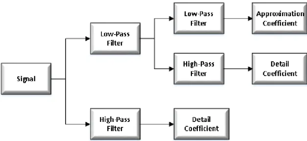
Unlike the Fourier transform, the wavelet transform has the ability to capture both low pass and high pass behaviors of an image. This property has proved very useful in image compression. From an image compression point of view, computational efficiency is an important factor to be considered. Fortunately, unlike DCT, DWT can be implemented as a fast algorithm via subband coding scheme. Typically, Discrete Wavelet Transform starts with the lowest scale (lowest level), corresponding to the given image, and computes the DWT coefficients by iterating the filtering and subsampling processes. This results in one approximation and many detail coefficients, as seen in Figure 2. It has been
observed in [15] from examples, that most of the energy of the DWT coefficients is packed in the approximation coefficients, which is a factor in achieving higher compression.
The Discrete Wavelet Transform represents an image as a sum of wavelet functions, known as wavelets, with different location and scale [15]. It represents the data into a set of high pass (detail) and low pass (approximate) coefficients. The input data is passed through set of low pass and high pass filters as described in Figure 2.
Figure 2: Process of a two level signal decomposition using multi-resolution analysis.
2.4.1 Haar transform – based image compression system
In order to fulfill the purpose of this thesis, the focus will be the Haar wavelet transform, also known as Daubechies D2 wavelet, presenting an all-optical image processing scheme based on it. The Haar wavelet transformation is an example of multi-resolution analysis. The purpose of this thesis is to use the Haar wavelet basis to compress an image data using the method of averaging and differencing to construct it. The simple Haar wavelet transformation matrix is given by Equation (2.1):
𝐻𝑎𝑎𝑟 𝑡𝑟𝑎𝑛𝑠𝑓𝑜𝑟𝑚𝑎𝑡𝑖𝑜𝑛 𝑚𝑎𝑡𝑟𝑖𝑥 = [ 1 √2 1 √2 1 √2 − 1 √2 ] (2.1)
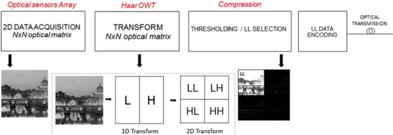
The system and building blocks used to process image were based on the described system building blocks and equations reported in [16] and [17], demonstrated in Figure 3.
Figure 3: System building blocks for Haar optical wavelet transform (OWT) based on all-optical processing and compression. 2D transform process schematic describes low-pass (L) and
high-pass (H) filtering until sub-band decomposition [16].
The system described in Figure 3 is a Haar all-optical wavelet transform (OWT), allowing fast image processing, with four main blocks:
Optical sensors array: this is the first building block, the acquisition stage with optical sensors for light detection and 2D data sampling to obtain an optical input data matrix with the same size 𝑁 × 𝑁 of the original image; Haar OWT: the second building block will be responsible for applying the
Haar transform to the image 𝑁 × 𝑁 obtained in the previous block, extracting the image properties obtained from exploiting the energy compaction features of wavelet decomposition. In this block, a matrix 𝑁 × 𝑁 will be applied based on Equation (2.2), the corresponding Haar Transform scattering matrix for a generic 1D input (ai coefficients), which
might be one pixel line or pixel column. This matrix includes the low-pass (L) and high-pass (H) filters associated with the Haar wavelet, that will be applied two times, one to obtain the 1D Transform (L and H component), and another to obtain the desirable 2D Transform with the four resulting
components, LL, LH, HL and HH. The resulting coefficients on the left side of Equation (2.2) are the scaling cij and detail dij coefficients (being i the
transform level and j the coefficients index) obtained from the low-pass and high-pass filtering, respectively, of each pixel pair, and corresponding to the 1D first level Haar discrete wavelet transform;
[ ⋮ 𝑐10 𝑑10 𝑐11 𝑑11 𝑐12 𝑑12 ⋮ ] = 1 √2 [ ⋯ ⋯ ⋯ 1 1 0 1 −1 0 0 0 1 ⋮ 0 0 0 0 0 0 1 0 0 ⋮ 0 0 1 0 0 0 0 0 0 ⋯ −1 0 0 0 1 1 0 1 −1 ⋯ ⋯ ][ ⋮ 𝑎0 𝑎1 𝑎2 𝑎3 𝑎4 𝑎5 ⋮ ] (2.2)
Compression: the aim of the third block is to compress and extract the desirable information from the 2D transform. In this block, the data will be quantized, reducing precision and specific components will be extracted, for example, the LL component;
LL data encoding: the last block will adapt the image data for the optical channel, compressing the data coding and bit stream formation.
On the receiver, after the optical channel, an inverse system will perform all the inverse transforms provided by the blocks on Figure 3, decoding the bit stream, de-quantized and then apply the inverse Haar transform on the data, returning the image able to be displayed.
2.4.2 Optical Haar transform device
To accomplish the Haar transform, the optical device choice must be one that accomplishes the scattering matrix from Equation (2.1), averaging and differentiating each optical input pair, as seen in Figure 4. Knowing that, the chosen device was a monomode 3dB asymmetric coupler, also known as Magic-T. An asymmetric coupler is a coupler with different waveguide widths, which might have a wide range of coupling ratios and low value of excess loss (0.7dB), including input and output single-mode fiber coupling losses [18]. In the case of
this thesis, since the asymmetric coupler must be arranged with not only a 50% coupling ratio, but also a phase difference between waveguides, a waveguide-type optical π hybrid coupler will be designed according to [16] and [19].
Figure 4: 3 dB asymmetric optical coupler scheme and scattering matrix [16].
Starting from the principle displayed in Figure 4 for a 1D transform, a 2D transform device will be designed, creating a three dimensional basic module, as shown in Figure 5. This device will implement the Low and High filtering one dimension a time, producing the scattering matrix given by Equation (2.2). From a 2 by 2 input matrix, with coefficients a0, a1, a2 and a3, the first two Magic-T will produce the
first high-pass and low-pass filtering along one dimension, the horizontal values. After this, the values will pass again by other two Magic-T, applying again the high-pass and low-pass filtering along the other dimension, the vertical values. With this, the scaling coefficients cij and detail coefficients dij will be obtained,
corresponding to the first level Haar DWT.
In this case of 2D processing, i is related to the filtering step on each dimension, while j is, again, the coefficients index.
With the device from Figure 5, the input data set can be increased, pilling and joining the basic module, creating a three dimensional integrated passive scheme for all-optical DWT with size 𝑁 × 𝑁 as shown in Figure 6. Figure 6 describes an 8 by 8 data input performing a second level wavelet transform.
Figure 6: Integrated passive scheme for Optical WT-IWT; passive compression is accomplished by spatial selection of the LL coefficients, delivered through reported connections [16].
For this device, only lossy compression method was considered, discarding some of the components and delivering to the Inverse transform block a reduced amount of information selected through a compression criterion.
Since the human eye is more sensitive to contrast changes while keeping the brightness differences, than to color changes [21], applying the wavelet transform will allow selecting the portion of the spectrum more sensitive to the human eye, the low frequency (LL) component. Reducing or eliminating the high frequency components will allow it to obtain compression, while keeping the most relevant information for the human eye.
Therefore, in order to implement compression, the possibility of using lossy compression will be considered, delivering only the lower frequency (LL) components using a guided and passive scheme. This approach will be tested on the mathematical software Matlab, selecting only the LL components, the
same transform block described in Figure 6, where only the low-frequency coefficients will propagate along active connections (lossy compression), accomplishing a passive selection for compression purposes.
2.5 Image quality assessment parameters
For the purpose of image analysis, the following quality assessment parameters will be used in this work. The simplest and most widely used full-reference quality metrics are:
MSE: the Mean Square Error is one way to evaluate the difference between an obtained value and the true value of the pixel obtained. MSE measures the average of the square of the error, with the error being the amount by which the estimator differs from the quantity to be estimated. The MSE between two images f and g is defined by Equation (2.3), in pixels: 𝑴𝑺𝑬 = 𝟏 𝑵∑ (𝒇[𝒋, 𝒌] − 𝒈[𝒋, 𝒌]) 𝟐 𝒋,𝒌 (2.3)
Where the sum over j, k denotes the sum over all pixels in the images and N is the number of pixels in each image. The closer the value of the MSE is to zero, the smaller the value of the error is and more similar is the compressed image to the original;
PSNR: In Peak Signal to Noise Ratio, the square of the peak value in the image is taken (in case of an 8-bit image, the peak value is 255) and divided by the Mean Square Error. The PSNR is used to measure the quality of an image after being submitted to a transformation. The PSNR between two (8 bpp) images is defined by Equation (2.4), in decibels (dB):
𝑷𝑺𝑵𝑹 = 𝟏𝟎 𝐥𝐨𝐠𝟏𝟎( 𝟐𝟓𝟓𝟐
𝑴𝑺𝑬) (2.4)
PSNR tends to be cited more often, since it is a logarithmic measure, and our brains seem to respond logarithmically to intensity. Increasing PSNR
represents increasing fidelity of compression. Generally, when the PSNR is between 30 dB and 40 dB, then the two images are virtually indistinguishable by human observers. When both images are identical (MSE of zero pixel), the PSNR is undefined, which in this case, to represent it graphically, the value of 99dB will be used.
These formulas are appealing because they are simple to calculate, have clear physical meanings, and are mathematically convenient in the context of optimization. However, they are not very well matched to perceived visual quality. For that, an additional quality assessment parameter will also be used:
Quality: Universal Image Quality Index is a formula based on [20], which instead of using the traditional error summation methods, like MSE and PSNR, is designed by modeling the image distortion as a combination of loss correlation, luminance distortion and contrast distortion.
If 𝒙 = {𝒙𝒊} is the original image and 𝒚 = {𝒚𝒊} is the test image, with 𝒊 = {𝟏, 𝟐, … , 𝑵}, the quality index is defined by Equation (2.5):
𝑄𝑢𝑎𝑙𝑖𝑡𝑦 = 4𝜎𝑥𝑦𝑥̅𝑦̅ (𝜎𝑥2+𝜎𝑥2)[(𝑥̅)2+(𝑦̅)2] (2.5) Where 𝑥̅ = 1 𝑁∑ 𝑥𝑖 𝑁 𝑖=1 , 𝑦̅ = 1 𝑁∑ 𝑦𝑖 𝑁 𝑖=1 , 𝜎𝑥2 = 1 𝑁−1∑ (𝑥𝑖 − 𝑥̅) 2 𝑁 𝑖=1 , 𝜎𝑦2 = 1 𝑁−1∑ (𝑦𝑖− 𝑦̅) 2 𝑁 𝑖=1 , 𝜎𝑥𝑦 = 1 𝑁−1∑ (𝑥𝑖 − 𝑥̅) 𝑁 𝑖=1 (𝑦𝑖− 𝑦̅)
The parameter Quality has a dynamic range from [-1, 1], with 1 being the best value where the obtained image is equal to the original and -1 being the lowest value achieved.
In evaluating the performance of any new image compression algorithm, one must take into account not only MSE, PSNR and Quality values, but also consider the following factors:
Perceptual quality of the images (visual difference of the original image and the compressed image);
Whether the algorithm allows for progressive transmission; The complexity of the algorithm (including memory usage);
Whether the algorithm has ROI (Region of Interest) capability.
In addition, in order to compare the amount of compression obtained by a compression method, the size (occupied space on the hard drive) of two images will be compared, in this case, the compressed image and the uncompressed image. The parameter Compression Ratio will be given by Equation (2.6):
𝐶𝑜𝑚𝑝𝑟𝑒𝑠𝑠𝑖𝑜𝑛 𝑟𝑎𝑡𝑖𝑜 = 𝑠𝑖𝑧𝑒 𝑜𝑓 𝑜𝑟𝑖𝑔𝑖𝑛𝑎𝑙 𝑖𝑚𝑎𝑔𝑒
𝑠𝑖𝑧𝑒 𝑜𝑓 𝑐𝑜𝑚𝑝𝑟𝑒𝑠𝑠𝑒𝑑 𝑖𝑚𝑎𝑔𝑒 (2.6)
In this case, if a compression ratio of 4 is obtained, the value is displayed “4:1”, which means that the compressed image is four times smaller than the original image.
Chapter 3: Theoretical implementation of the optical system
in Matlab
3.1 Implementation of the Haar wavelet transform
To implement theoretically the Haar wavelet transform, the mathematical software MATLAB was used to compress and analyze the image data.
To do that, several types of images were used with different formats (TIF, JPEG, BMP and PNG), all of them square images with the same number of lines and columns (as seen in Chapter 2.4, the Haar transformation matrix is a square matrix) and all of them in the grayscale color space.
The reason to use only grayscale images was to simplify the analysis, since the main difference for this case, is that instead of having three colors like in the RGB color space (Red, Green and Blue), it has only one.
Finally, the reason to use four types of image formats was that all image formats (TIF, JPEG, BMP and PNG) are different: some lossless, other lossy, all with different characteristics that will differ after being affected by the Haar wavelet transform. This is important because in some cases, the transformation will be more significant and in other cases, the transformation will have much less effect. The characteristics of the images used in this chapter are listed in Table 1.
Name Figure in Attachments Format Color space Size (kB) Size (Rows x Columns) TIF - 1 Figure 63 TIF Grayscale 265 512 x 512 TIF - 2 Figure 66 TIF Grayscale 65 256 x 256 TIF - 3 Figure 69 TIF Grayscale 1 040 1024 x 1024 TIF - 4 Figure 72 TIF Grayscale 31 688 x 688 JPEG - 1 Figure 75 JPG Grayscale 1 564 2832 x 1832 JPEG - 2 Figure 78 JPG Grayscale 338 2832 x 2832 JPEG - 3 Figure 81 JPG Grayscale 857 2832 x 2832 JPEG - 4 Figure 84 JPG Grayscale 599 2832 x 2832 BMP - 1 Figure 87 BMP Grayscale 263 512 x 512 BMP - 2 Figure 90 BMP Grayscale 67 256 x 256 BMP - 3 Figure 93 BMP Grayscale 41 200 x 200 BMP - 4 Figure 96 BMP Grayscale 361 600 x 600 PNG - 1 Figure 99 PNG Grayscale 61 300 x 300 PNG - 2 Figure 102 PNG Grayscale 63 512 x 512 PNG - 3 Figure 105 PNG Grayscale 483 1001 x 1001 PNG - 4 Figure 108 PNG Grayscale 198 512 x 512
Table 1: Characteristics of the images used for comparison.
To start the Haar wavelet transform, an “Original image” with size 𝑵 × 𝑵, was multiplied 2 times by the “Haar transformation matrix” with size 𝑵 × 𝑵 (applied to the rows and column) to obtain the “Haar transform image”. The “Haar transform image” contains the “Scaling image”, “Horizontal details image”, “Vertical details image” and “Diagonal details image”, which in this step a lossless compression method is obtained, that means, it is possible to redo the transform and obtain the original image exactly as it was (first step of Figure 7).
To increase the amount of compression, with the “Haar transform image”, it is possible to extract the “Scaling image”, which is an image much similar to the original, but with size 𝑵
𝟐× 𝑵
𝟐. In this case, the compression method is lossy, since
from only the “Scaling image”, it is not possible to retrieve the original image. The previous steps can be seen in Figure 7.
Figure 7: Haar wavelet transform applied to the image "TIF-1".
3.1.1 Lossless compression
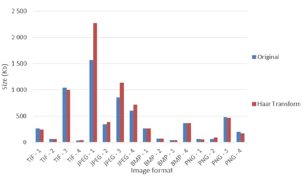
To analyze the lossless compression method in Matlab, the size (occupied space on the hard drive) of the original image was compared with the resulting image of the Haar transform. The results can be seen in Figure 8.
Figure 8: Size and image format comparison in lossless compression.
As seen in Figure 8, the lossless compression of the Haar transform might be useful in the lossless compression methods, like TIF, BMP and PNG, producing images approximately 8% smaller than the original. However, in the case of the JPEG lossy compression method, since the image was already highly compressed, the resulting image from the Haar transform is larger than the original, introducing redundancy in the output.
3.1.2 Lossy compression
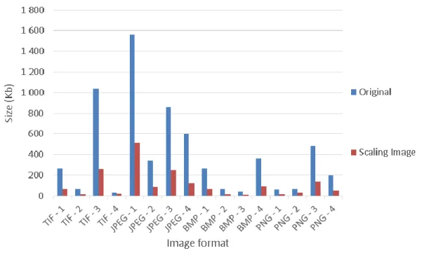
After the lossless compression, the lossy compression method will be analyzed in Matlab, comparing the size (occupied space on the hard drive) of the original image with the Scaling image resulting from the Haar transform. The results can be seen in Figure 9.
Figure 9: Size and image format comparison in lossy compression.
As seen in Figure 9, the lossy compression method of the Scaling image is able to compress all the image’s formats, lossy or lossless, but with the cost of losing quality and a resulting image with half the rows and columns of the original image. In Figure 10, with the values from Figure 8 and Figure 9, the compression ratios of the Haar transform and Scaling image were calculated in order to visualize the amount of compression able to obtain with each one of the methods.
Figure 10: Compression ratio and file format of the image. Comparison by compression method.
From Figure 10, it is clear that with the lossy compression method of the Scaling image, it is possible to obtain an average compression ratio around 4:1 and with the lossless method of the Haar transform, the average compression ratio is about 1:1, which means that when the size of the image is not important, and high compression ratio is required, lossy compression method can be advantageous.
3.1.2.1 Lossy compression with variation in the amplitude of the parameters of the Haar transformation matrix
In this chapter, the amplitude of the Haar transformation matrix parameters were changed, in order to analyze the effect of loss in the parameters of a real device used in the laboratory, to obtain only the Scaling image.
Five different configurations were used to simulate the transformation, changing the amplitude from 0.088 to 1.1414. There is one configuration with all the parameters of Equation (3.1) changing in the same amplitude, and four configurations changing each one of the four parameters from Equation (3.1) and maintaining the remaining parameters from Equation (2.1) unchanged.
𝐵𝑎𝑠𝑖𝑐 𝐻𝑎𝑎𝑟 𝑡𝑟𝑎𝑛𝑠𝑓𝑜𝑟𝑚𝑎𝑡𝑖𝑜𝑛 𝑚𝑎𝑡𝑟𝑖𝑥 = [1𝑠𝑡 2𝑛𝑑
3𝑟𝑑 4𝑡ℎ] (3.1)
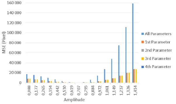
To compare the effect of the parameters, three image quality assessment parameters were used: MSE, PSNR and Quality, Figure 11, Figure 12 and Figure 13 respectively.
Figure 11: MSE and amplitude variation in the Haar transform matrix comparison.
In Figure 11, it is possible to observe that when it comes to the MSE, the most significant output is when all the parameters are affected by an error, obtaining the highest values of MSE. The other two parameters that affect the Scaling image are the first and the third parameters, still affecting considerably the output image outside the rage of values between 0.530 and 0.884. The second or forth parameter do not affect in any way the output of the Scaling image.
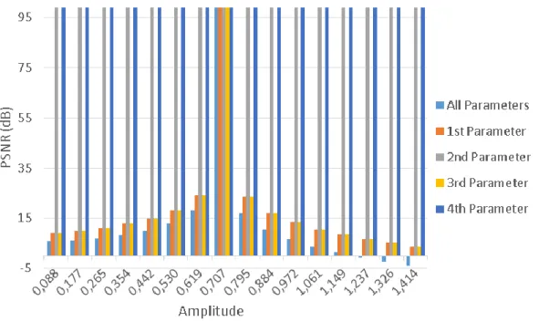
Figure 12: PNSR and amplitude variation in the Haar transform matrix comparison.
In Figure 12, it is possible to observe that the effect of the parameters on the PSNR is much likely as the effect on the MSE. When the second or forth parameters are affected or a value of 0.707 (1
√2) is obtained, the Scaling image is
not affected at all (PSNR of 99dB). If the values diverge from 0.707, increasing or lowering, the Scaling image is affected and the values of the PSNR start decreasing. The PSNR decreases more when all the parameters are affected.
Figure 13: Quality and amplitude variation in the Haar transform matrix comparison.
Finally, in Figure 13, the deductions from Figure 11 and Figure 12 are verified, where besides the findings in the previous figures of MSE and PSNR, outside the rage of values between 0.530 and 0.884, the Quality of the image decreases below 0.9, which is a significant perceptual difference in the Scaling image.
3.1.2.2 Lossy compression with variation in the phase of the parameters of the Haar transformation matrix
In this chapter, the phase of the Haar transformation matrix parameters were changed, in order to analyze the effect of loss in the parameters of a real device used in the laboratory.
Five different configurations were used to simulate, changing from -90 degrees to 90 degrees. There is one configuration with all the phase parameters of Equation (3.1) changing in the same amplitude of phase, and four configurations changing each one of the 4 parameters from Equation (3.1) and maintaining the remaining phase parameters from Equation (3.2) unchanged.
𝐻𝑎𝑎𝑟 𝑡𝑟𝑎𝑛𝑠𝑓𝑜𝑟𝑚𝑎𝑡𝑖𝑜𝑛 𝑚𝑎𝑡𝑟𝑖𝑥 = [ 1 √2cos(0°) 1 √2cos(0°) 1 √2cos(0°) 1 √2cos(180°) ] (3.2)
To compare the effects, the same three image quality assessment parameters from the last chapter were used: MSE, PSNR and Quality, Figure 14, Figure 15 and Figure 16 respectively.
Figure 14: MSE and phase variation in the Haar transform matrix comparison.
In Figure 14, it is possible to observe that when it comes to the MSE, the most significant output is when all the parameters are affected by an error in the phase, obtaining the highest values of MSE. The other two parameters that affect the Scaling image are the first and the third parameters, still affecting considerably the output image outside the rage of values between -45° and -45°. The second or forth parameter do not affect in any way the output of the Scaling image.
Figure 15: PNSR and phase variation in the Haar transform matrix comparison.
In Figure 15, it is possible to observe that the effect of the parameters on the PSNR is much likely as the effect on the MSE. When the second or forth parameter are affected or a phase difference of 0° is obtained, the Scaling image is not affected at all (PSNR of 99dB). If the phase diverges from 0°, increasing or lowering, the Scaling image is affected and the values of the PSNR start decreasing. The PSNR decreases more when all the parameters are affected.
Finally, in Figure 16, the deductions from Figure 14 and Figure 15 can be verified, where besides the findings in the previous figures of MSE and PSNR, outside the rage of values between -45° and -45°, the Quality of the image decreases below 0.9, which is a significant perceptual difference in the Scaling image.
3.2 Implementation of additional compression in the data
encoding process
As seen in Chapter 2.4, after the Haar transformation block, it is possible to increase the data transmission by a thresholding or quantization method before the optical transmission, where the number of symbols necessary to encode will be reduced, increasing the data transmission speed.
To analyze these methods, the mathematical software MATLAB was used to compress and analyze the image TIF 1 (Figure 63 from Attachments) after lossless compression: first by a thresholding method, then with a quantization method. The analysis was directed to the lossless compression due to the high quantity of zero values presented in the details coefficients in the Haar transform image (Figure 64 from Attachments), which is the one that will be transmitted in the optical transmission channel in this case.
3.2.1 Additional compression with threshold
In this part, additional compression will be added by a thresholding method. Image threshold is a simple, yet effective way of reducing the number of symbols necessary to encode an image.
This method sets all the negative pixel, and below a certain amount threshold with the value zero. With this, the necessary symbols to encode those amounts were eliminated.
For example, an image with the pixel’s values of 56, 200, 8 and 0, before thresholding, four sets of symbols were needed to encode that image (56, 200, 8
and 0). If a thresholding of 50 was applied, only three sets of symbols would be needed (56, 200, and 0), eliminating the symbol necessary to encode pixel 8. Seven levels of thresholding were used (0, 4, 8, 16, 32, 64 and 128), where in the first level (0) only the negative values were made equal to zero. In the remaining levels (4, 8, 16, 32, 64 and 128), they were already submitted to some amount of thresholding. For example, with the threshold level 8, the symbols necessary to encode the negative pixels and the pixels from 1 to 7 were eliminated.
The obtained images after applying the threshold 0, 4, 8, 16, 32, 64 and 128 can be seen in the chapter Attachment, Figure 111, Figure 112, Figure 113, Figure 114, Figure115, Figure 116 and Figure 117 respectively.
Figure 17: Number of occurrences of each pixel (symbol) by level of threshold
From Figure 17, it is possible to say that, higher the threshold submitted to the image, higher the number of occurrences of the value zero. In addition, while the threshold is increased, the lower values (threshold of 0, 4, 8 and 16) tend to lower exponentially the number of occurrences, which are the ones that are being turn into zero. By the analysis of this figure (17), the expected result is confirmed, which is a lower number of symbols in the image, turning the values lower than a threshold equal to zero.
Level of threshold MSE (pixel) PSNR (dB) Quality 0 22.04 34.70 0.90 4 22.05 34.70 0.90 8 22.18 34.67 0.90 16 22.91 34.53 0.86 32 25.68 34.03 0.82 64 440.22 21.69 0.69 128 3976.00 12.14 0.37
Table 2: Quality assessment parameters by level of threshold
From Table 2 and the figures in the chapter Attachment (Figure 111, Figure 112, Figure 113, Figure 114, Figure 115, Figure 116 and Figure 117), until the threshold value of 32, the image does not show much loss of quality, obtaining a quality assessment parameters of 25.68 pixels for the MSE, 34.03 dB of PSNR and 0.82 of Quality. This method has proven to be a very good way to increase the data transmission speed of the Haar transform image in the optical transmission channel.
3.2.2 Additional compression with quantization
In this chapter, additional compression will be added by a quantization method. Image quantization is another simple way of reducing the number of symbols necessary to encode an image.
This method sets all the negative pixel equal to zero and the positive values are rounded to the nearest multiple of quantization’s value. With this, the necessary symbols to encode those amounts were eliminated.
For example, an image with the pixel’s values of 56, 200, 8 and 0, before quantization, four sets of symbols to encode that image were needed (56, 200, 8 and 0). If a quantization value of 100 was applied, only three sets of symbols would be needed (100, 200, and 0), eliminating the symbol necessary to encode pixel 8.
Six levels of quantization were used (1, 2, 5, 10, 20 and 50), where in the first level (1) only the negative values were made equal to zero. In the remaining levels (2, 5, 10, 20 and 50), they were already submitted to some amount of quantization. For example, from the quantization level 2, only approximately half of the symbols are needed to encode the image comparing to the quantization level 1.
The obtained images after applying the quantization 1, 2, 5, 10, 20 and 50 can be seen in the chapter Attachment, Figure 118, Figure 119, Figure 120, Figure 121, Figure 122 and Figure 123 respectively.
Figure 18: Number of occurrences of each pixel (symbol) by level of quantization
From Figure 18, it is possible to say that, higher the quantization submitted to the image, higher the number of occurrences of value zero, but still lower than the values obtained from the previous threshold method. Also, while the quantization value is increased, higher are the occurrences of the values along the horizontal scale of Figure 18. By the analysis of this figure, the expected result is confirmed, which is an increase of the values that are multiple to the quantization value, reducing the amount of symbols between two multiples of the quantization.
Level of quantization MSE (pixel) PSNR (dB) Quality 1 21.86 34.73 0.90 2 22.25 34.66 0.90 5 23.91 34.35 0.86 10 30.45 33.29 0.77 20 55.94 30.65 0.65 50 198.21 25.16 0.39
Table 3: Quality assessment parameters by level of quantization
From Table 3 and the figures in the chapter Attachment (Figure 118, Figure 119, Figure 120, Figure 121, Figure 122 and Figure 123), until the quantization value of 5, the image does not show much loss of quality, obtaining a quality assessment parameters of 23.91 pixels for the MSE, 34.35 dB of PSNR and 0.86 of Quality. This method has proven to be a very good way to increase the data transmission speed of the Haar transform image in the optical transmission channel.
Chapter 4: Laboratory experiment with the Haar wavelet
transform
In this chapter, the Haar Wavelet transform was simulated in the laboratory using the available devices. Two wavelength with distinct characteristics were chosen to verify the dependency of the wavelength in the experiment, with different optical lasers, components and measurement equipment.
The first wavelength used was the 635 nm, a visible red laser to the human observer. The second wavelength used was the 1550 nm, which, contrary to the wavelength of 635 nm, is not visible to the human eye.
4.1 Visible spectral region (635 nm wavelength)
To accomplish the experiment in the visible spectral region (635 nm), two small portions of the grayscale image “TIF-1” (Figure 63 from Attachments) were extracted, with a size of 4x4 pixel to compare in terms of contrast: one with moderate contrast and one with higher level of contrast, Figure 19 and Figure 20 respectively.
Figure 19: Image 4x4 with moderate contrast. Figure 20: Image 4x4 with high contrast.
4.1.1 Setup
First, to start the experiment, the pixel value of the images were converted to a power scale (dBm), maximizing the power range available from the red lasers.
The ranges used in the experiment are listed in Table 4 for each one of the schemes used. Image Unit Moderate contrast image with Coupler 1 (scheme 1) Moderate contrast image with Coupler 2 (scheme 2) High contrast image with Coupler 2 (scheme 3) Pixel Lower value 55 55 53 Higher value 202 202 223 dBm Lower value -24.1 -24.1 -24.0 Higher value -17.5 -17.5 -18.0
Table 4: Power range used with the 3dB coupler setup.
Secondly, two different setups with two different images were used to compare results. One of the setups (scheme 1) was assembled with a two input, two output 3dB coupler for the 635 nm wavelength with the following coupling coefficients:
Input 1 – Output 1: 50.6%; Input 1 – Output 2: 49.4%; Input 2 – Output 1: 48.8%; Input 2 – Output 2: 51.2%.
The second setup (scheme 2 and scheme 3) was assembled with a different two input, two output 3dB coupler for the 635 nm wavelength with the following coupling coefficients:
Input 1 – Output 1: 52.2%; Input 1 – Output 2: 47.8%; Input 2 – Output 1: 49.1%; Input 2 – Output 2: 50.9%.
The rest of the components were common to each one of the setups: 2 Red lasers with different power ranges;
1 Power meter.
The described setup can be seen in Figure 21 and Figure 22.
Figure 21: Setup with a 3dB coupler.
Figure 22: Photography of the 635 nm setup.
Next, with the pixel’s values converted to the power scale (dBm):
First, those values were regulated in the input of the 3dB coupler in groups of two horizontal values and obtained the vertical transform (L component of the Haar wavelet transform). The experiment was repeated 3 times; Secondly, the values obtained in the previous paragraph were adjusted
again in groups of 2 vertical values, obtaining the final LL component (Scaling image of the Haar wavelet transform).
4.1.2 Results
To analyze the results, besides the parameters already discussed in Chapter 2.5, two more parameters were used regarding the experience in the laboratory:
Insertion Loss (IL): an average parameter, obtained by dividing the obtained value of the pixels by their theoretical value. The meaning of this parameter is that since most of the components used in the laboratory have a percentage of loss in this operation, if the Insertion Loss is constant during the experiment, that value of loss is possible to compensate in the receiver canceling that loss. This value will be multiplied again by the obtained pixel to analyze the result of the component’s loss in the experiment;
Average Standard Deviation: an average value of the standard deviation calculated by discrepancy of the pixel in the output of the coupler in the repetition of the experiment 3 times. This parameter is used to verify the insertion of loss during the experiment while connecting and disconnecting the fibers. The lower the value obtained, the better the experiment will be.
Insertion Loss (pixel) Average Standard Deviation (pixel) MSE (pixel) PSNR (dB) Scheme 1 7.95±12.33 1.99 9611.2 8.3 Scheme 1 with IL 9476.8 8.4 Scheme 2 26.19±61.93 4.69 10839.5 7.8 Scheme 2 with IL 10815.5 7.8 Scheme 3 71.35±168.58 2.42 26860 3.8 Scheme 3 with IL 4919 11.2
Table 5: Schemes comparison for the 635 nm wavelength.
From Table 5, looking to the obtained values of the parameter Insertion Loss, it is possible to say that the obtained pixel, even without considering the loss in the components, will be very different from the original values, since the minimum deviation is around 12 pixel. This results are verified in the obtained values of MSE and PSNR, where with or without considering the IL (Insertion Loss parameter), the MSE is extremely high and the PSNR is very low, expecting
images very different from the originals. From the values obtained in the Average Standard Deviation, in the case of the 635 nm wavelength, it is possible to say that, the process of connecting and disconnecting the fibers, introduces some error, from about 2 to 4 pixel.
4.1.3 Image comparison
In this chapter, the images will be compared using the human eye perception, comparing the theoretical Scaling image with each one of the obtained Scaling images. Two obtained Scaling images will be displayed, one that was multiplied by the obtained value of Insertion Loss to try to cancel the value of loss in the components (with IL) and other exactly as it was obtained (without IL).
4.1.3.1 4x4 Image with moderate contrast:
Figure 23: Theoretical Scaling image.
Figure 24: Obtained Scaling image from scheme 1 with IL.
Figure 25: Obtained Scaling image from scheme 1 without IL.
Comparing the theoretical Scaling image (Figure 23) with the obtained images (Figure 24 and Figure 25), it is possible to confirm the deductions made in chapter 4.1.2, where the images obtained with scheme 1 are both (with and without IL) very different from the theoretical, being the obtained image without IL the one with similar contrast but much darker.
Figure 26: Obtained Scaling image from scheme 2 with IL.
Figure 27: Obtained Scaling image from scheme 2 without IL.
Looking to Figure 26 and Figure 27, the deductions made from Figure 24 and Figure 25 are also proven, where both images are very different from the theoretical.
4.2.3.2 4x4 Image with high contrast:
![Figure 1: Data growth by year [2].](https://thumb-eu.123doks.com/thumbv2/123dok_br/15747192.1073256/27.892.186.712.622.891/figure-data-growth-by-year.webp)
![Figure 6: Integrated passive scheme for Optical WT-IWT; passive compression is accomplished by spatial selection of the LL coefficients, delivered through reported connections [16]](https://thumb-eu.123doks.com/thumbv2/123dok_br/15747192.1073256/40.892.237.654.330.645/integrated-optical-compression-accomplished-selection-coefficients-delivered-connections.webp)