Susana
de Jesus Mota
Modelos de Canal para Sistemas MIMO
Susana
de Jesus Mota
Modelos de Canal para Sistemas MIMO
Channel Modeling for MIMO Systems
Tese apresentada à Universidade de Aveiro para cumprimento dos requisitos necessários à obtenção do grau de Doutor em Engenharia Eletrotécnica, realizada sob a orientação científica do Doutor Armando Carlos Domingues da Rocha, Professor Auxiliar do Departamento de Eletrónica, Telecomunicações e Informática da Universidade de Aveiro
À minha família
“Alea jacta est ”
o júri
presidente Doutor Vítor José Babau Torres
Professor Catedrático da Universidade de Aveiro
Doutor Francisco António Bucho Cercas
Professor Catedrático do ISCTE-IUL – Instituto Universitário de Lisboa
Doutor Fernando Pérez-Fontán
Professor Catedrático da Universidade de Vigo
Doutor João Nuno Pimentel Silva Matos
Professor Associado da Universidade de Aveiro
Doutor Fernando José da Silva Velez
Professor Auxiliar da Universidade da Beira Interior
Doutor Armando Carlos Domingues da Rocha
agradecimentos Ao Prof. Doutor Armando Rocha, meu orientador, pelo apoio, pela disponibilidade, pelo aconselhamento, pela sua orientação afinada e focalizada evitando desvios vãos, por todos os esforços que desenvolveu e acima de tudo, pela paciência e compreensão. Devo também pela sua iniciativa de solicitar a colaboração do Prof. Doutor Fernando Pérez-Fontán da Universidade de Vigo, Espanha.
Ao Prof. Doutor Fernando Pérez-Fontán, por me ter acolhido tão prontamente e cordialmente, pelas discussões proveitosas que mantivemos, pelas sugestões, pela motivação que sempre me transmitiu e ainda por todo o empenho que mostrou para tornar possíveis as reuniões que fomos mantendo periodicamente.
Ao Instituto de Telecomunicações – polo de Aveiro, pelas condições de trabalho que me proporcionou.
A toda a equipa técnica do Instituto de Telecomunicações, por todo apoio prestado, especialmente ao Miguel Lacerda e ao Paulo Gonçalves pelo apoio durante as campanhas de medidas.
À Fundação para a Ciência e Tecnologia (FCT), pela bolsa concedida (Ref.ª SFRH / BD / 6418 / 2001).
À minha família, em especial ao meu marido, à minha filha, aos meus pais, à minha irmã e ao meu cunhado pelo apoio contínuo.
Também a todos os meus amigos pelo facto de o serem, mas em especial ao amigo Lucénio pelo seu apoio, pelo seus esforços e pela confiança que em mim depositou.
palavras-chave Sistemas MIMO, Modelos de Canal, Multipercurso, Canal Rádio Direcional, Medidas Experimentais, Estimação Paramétrica, Classificação de Dados
resumo Os sistemas equipados com múltiplas antenas no emissor e no recetor, conhecidos como sistemas MIMO (Multiple Input Multiple Output), oferecem capacidades mais elevadas, permitindo melhor rentabilização do espectro e/ou utilização de aplicações mais exigentes. É sobejamente sabido que o canal rádio é caracterizado por propagação multipercurso, fenómeno considerado problemático e cuja mitigação tem sido conseguida através de técnicas como diversidade, formatação de feixe ou antenas adaptativas. Explorando convenientemente o domínio espacial os sistemas MIMO transformam as características multipercurso do canal numa mais-valia e permitem criar vários canais virtuais, paralelos e independentes. Contudo, os benefícios atingíveis são condicionados pelas características do canal de propagação, que poderão não ser sempre as ideais.
Este trabalho centra-se na caracterização do canal rádio para sistemas MIMO. Inicia-se com a apresentação dos resultados fundamentais da teoria da informação que despoletaram todo o entusiamo em torno deste tipo de sistemas, sendo discutidas algumas das suas potencialidades e uma revisão dos modelos existentes para sistemas MIMO.
A caracterização do canal MIMO desenvolvida neste trabalho assenta em medidas experimentais do canal direcional adquiridas em dupla via. O sistema de medida é baseado num analisador de redes vetorial e numa plataforma de posicionamento bidimensional, ambos controlados por um computador, permitindo obter a resposta em frequência do canal rádio nos vários pontos correspondentes à localização dos elementos de um agregado virtual. As medidas são posteriormente processadas com o algoritmo SAGE ( Space-Alternating Expectation-Maximization), de forma a obter os parâmetros (atraso, direção de chegada e amplitude complexa) das componentes multipercurso mais significativas. Seguidamente, estes dados são tratados com um algoritmo de classificação (clustering) e organizados em grupos. Finalmente é extraída informação estatística que permite caracterizar o comportamento das componentes multipercurso do canal.
A informação acerca das características multipercurso do canal, induzidas pelos espalhadores (scatterers) existentes no cenário de propagação, possibilita a caracterização do canal MIMO e assim avaliar o seu desempenho. O método foi por fim validado com medidas MIMO.
keywords MIMO Systems, Channel Models, Multipath, Diretional Radio Channel, Experimental Measurements, Parametric Estimation, Data Clustering
abstract Systems equipped with multiple antennas at the transmitter and at the receiver, known as MIMO (Multiple Input Multiple Output) systems, offer higher capacities, allowing an efficient exploitation of the available spectrum and/or the employment of more demanding applications. It is well known that the radio channel is characterized by multipath propagation, a phenomenon deemed problematic and whose mitigation has been achieved through techniques such as diversity, beamforming or adaptive antennas. By exploring conveniently the spatial domain MIMO systems turn the characteristics of the multipath channel into an advantage and allow creating multiple parallel and independent virtual channels. However, the achievable benefits are constrained by the propagation channel’s characteristics, which may not always be ideal.
This work focuses on the characterization of the MIMO radio channel. It begins with the presentation of the fundamental results from information theory that triggered the interest on these systems, including the discussion of some of their potential benefits and a review of the existing channel models for MIMO systems.
The characterization of the MIMO channel developed in this work is based on experimental measurements of the double-directional channel. The measurement system is based on a vector network analyzer and a two-dimensional positioning platform, both controlled by a computer, allowing the measurement of the channel’s frequency response at the locations of a synthetic array. Data is then processed using the SAGE (Space-Alternating Expectation-Maximization) algorithm to obtain the parameters (delay, direction of arrival and complex amplitude) of the channel’s most relevant multipath components. Afterwards, using a clustering algorithm these data are grouped into clusters. Finally, statistical information is extracted allowing the characterization of the channel’s multipath components.
The information about the multipath characteristics of the channel, induced by existing scatterers in the propagation scenario, enables the characterization of MIMO channel and thus to evaluate its performance. The method was finally validated using MIMO measurements.
Table of Contents
List of Figures ... xvii
List of Tables... xxiii
Notation and List of Symbols ... xxv
Acronyms ... xxix
1.
Introduction ... 1
2.
MIMO Wireless Communications ... 5
2.1. System Model ... 5
2.2. Capacity analysis ... 7
2.2.1. From Shannon to MIMO Systems Capacity ... 7
2.2.2. Eigenvalue Analysis of the Channel ... 8
2.2.3. Stochastic Channels ... 13
2.2.4. Frequency Selective Channels ... 14
2.3. MIMO Potentials ... 16
2.3.1. Beamforming ... 17
2.3.2. Spatial Diversity ... 17
2.3.3. Spatial Multiplexing ... 19
2.3.4. Transmission over MIMO systems ... 19
2.4. MIMO Channel Models ... 21
2.4.1. Brief review of propagation mechanisms ... 21
2.4.2. The double-directional channel impulse response... 22
2.4.3. Model Classification ... 24
2.4.4. Ray-based deterministic models ... 25
2.4.6. Empirical stochastic models ... 29
2.4.7. Standardized models ... 31
3.
SIMO Measurements and Estimation of the Directional Channel ... 37
3.1. The Wideband Radio Channel Characterization ... 37
3.1.1. Channel System Functions ... 38
3.1.2. Stochastic Description of the Channel ... 40
3.2. SIMO Setup and Measurement Campaign ... 42
3.3. Estimation of Superimposed Signals ... 43
3.3.1. High Resolution Algorithms ... 43
3.3.2. Signal Model ... 45
3.3.3. Maximum-Likelihood Estimation and the EM Algorithm ... 46
3.3.4. Description of the SAGE Algorithm ... 49
3.4. SAGE Results using Synthetic Data ... 52
3.5. Experimental DCIRs obtained with SAGE algorithm ... 56
4.
Exploratory Study of the Directional Channel Information ... 59
4.1. Brief Review of Clustering Algorithms... 60
4.2. Clustering of the Multipath Radio Channel Parameters ... 63
4.2.1. MPC Distance ... 64
4.2.2. KPM Algorithm ... 65
4.3. Clustering Validation ... 68
4.3.1. Validation Indices ... 69
4.3.2. Fusion Techniques ... 71
4.4. Clustering Results using Synthetic DCIRs ... 72
4.4.1. Preliminary Evaluation of the Clustering Framework ... 73
4.4.2. Structured Evaluation of the Clustering Framework ... 76
4.5. Summary of the Clustering Framework ... 79
4.6. Clustering Results using Real DCIRs ... 80
4.7. Physical Analysis of Clustered DCIRs ... 82
5.
MIMO Modeling and Measurements ... 87
5.1. Modeling Assumptions ... 87
5.2. Statistical Analysis of Clustered DCIRs ... 89
5.2.1. Inter-Cluster Analysis ... 90
5.2.2. Intra-Cluster Analysis ... 95
5.3. Channel Simulator Description ... 99
5.3.2. Generation of the Channel Scatterers (Step 3) ... 106
5.3.3. Generation of the traveled route(s) (Step4) ... 108
5.3.4. Obtaining the Frequency Responses Matrix Series (Step 5) ... 110
5.3.5. Simulator Sample Results ... 111
5.4. MIMO Measurement Campaign ... 115
5.5. Measurements Results vs Simulator Outputs ... 117
5.5.1. Assessment of the SISO Characterization ... 119
5.5.2. Assessment of the MIMO Characterization ... 122
5.6. Final Comments on the Modeling Methodology ... 124
6.
Conclusion ... 125
6.1. Final Remarks ... 126
6.2. Future Work ... 128
Appendix A.
Method for Generating Random Variables ... 129
Appendix B.
Simulator Sample Results: OLoS Channel ... 133
B.1. Channel MPCs and Scatterers ... 133
B.2. SISO Outputs ... 134
B.3. MIMO Outputs ... 135
Appendix C.
Measurements vs Simulations: Additional Results ... 137
C.1. Assessment of the SISO Characterization ... 137
C.2. Assessment of the MIMO Characterization ... 139
List of Figures
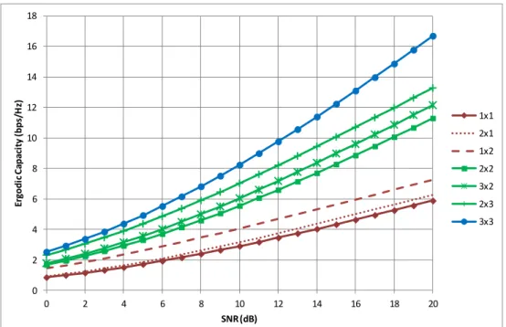
Figure 2-1: Schematic of MIMO system with Nt antennas at the transmitter and Nr antennas at the receiver. ... 6 Figure 2-2: Illustration of the water-filling algorithm. ... 12 Figure 2-3: Ergodic capacity for different antenna configurations: the curves labels
indicate Nt×Nr. ... 14 Figure 2-4: CDF of the information rate for an increasingly frequency selective
MIMO channel. ... 16 Figure 2-5: Equivalent scatterer (□) concept (true scatterers are represent by ○). ... 27 Figure 2-6: Exponential decay of the mean amplitude for clusters and for MPCs
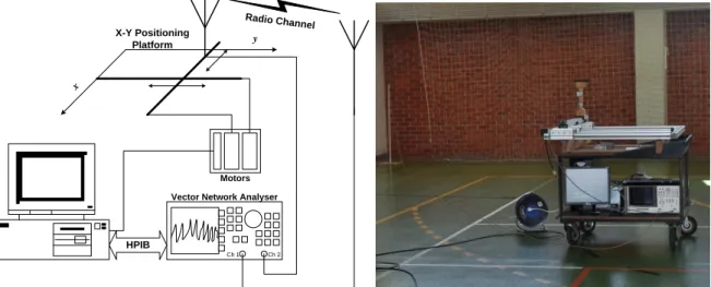
within clusters. ... 31 Figure 3-1: Block diagram and a photograph of the SIMO channel measurement
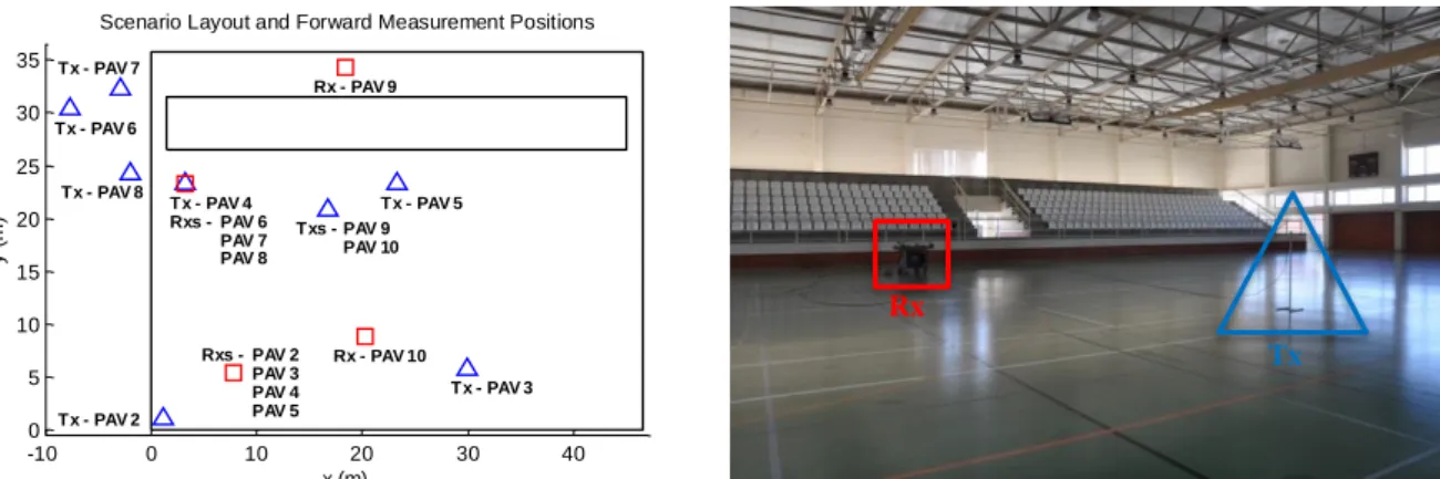
system. ... 42 Figure 3-2: Description of the forward measurement positions in the scenario and a
photograph corresponding to the reverse measurement position “PAV 10 rv”. ... 43 Figure 3-3: Relation between the complete data (unobservable) and the incomplete
data (observable). ... 47 Figure 3-4: Signal flowchart of the EM algorithm. ... 49 Figure 3-5: Signal flowchart of the SAGE algorithm. ... 51 Figure 3-6: SAGE retrieval results (15 estimates requested) for “ch4” (15 rays,
“moderate” power decay). Left: Generated impulse response and SAGE retrieval. Right: Reconstructed impulse responses by using IFFT on frequency responses obtained with equation (3.17). ... 53 Figure 3-7: Directional impulse responses (time and azimuth domains) for “ch4”.
Left: ESV generated impulse response. Right: SAGE retrieved impulse
Figure 3-8: SAGE retrieval results (50 estimates requested) for “ch9” (50 rays,
“moderate” power decay). Left: Generated impulse response and
SAGE retrieval. Right: Reconstructed impulse responses by using IFFT
on frequency responses obtained with equation (3.17). ... 54
Figure 3-9: Directional impulse responses (time and azimuth domains) for “ch9”. Left: ESV generated impulse response. Right: SAGE retrieved impulse response. ... 54
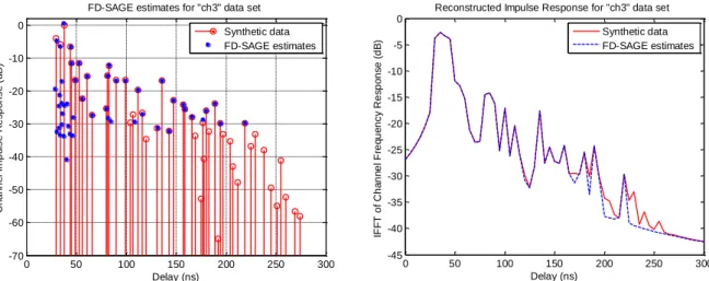
Figure 3-10: SAGE retrieval results (50 estimates requested) for “ch3” (50 rays, “pronounced” power decay). Left: Generated impulse response and SAGE retrieval. Right: Reconstructed impulse responses by using IFFT on frequency responses obtained with equation (3.17). ... 55
Figure 3-11: Directional impulse responses (time and azimuth domains) for “ch3”. Left: ESV generated impulse response. Right: SAGE retrieved impulse response. ... 55
Figure 3-12: Forward measurement results [PAV-10] – Left: Average impulse response obtained from measurements and SAGE output. Right: DCIR estimated by SAGE. ... 57
Figure 3-13: Reverse measurement results [PAV-10rv] – Left: Average IR obtained from measurements and SAGE output. Right: Directional IR estimated by SAGE. ... 57
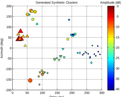
Figure 4-1: Sample of a synthetic channel generated, using the ESV model, with 7 clusters and 8 MPCs per cluster. ... 74
Figure 4-2: Comparison of final KPM partitions for K=7 using different initialization strategies. Left: MCD without power weight. Right: MCD with power weight. ... 74
Figure 4-3: Comparison of initialization strategies. Left: MCD without power weight. Right: MCD with power weight. ... 75
Figure 4-4: Cluster Validation for the data set of Figure 4-1 (Ktrue=7) with Kopt highlighted by a red circle. Left: Individual indices results. Right: Fusion techniques results. ... 76
Figure 4-5: KPM success rate. ... 78
Figure 4-6: CVI success rates. ... 78
Figure 4-7: Underestimation and overestimation rates for XB and D53. ... 78
Figure 4-8: Fusion techniques success rate. ... 79
Figure 4-9: Forward Measurement [PAV-10] – Left: Cluster validity results for each KPM solution. Right: Clustering solution that was selected for this experimental data set. ... 81
Figure 4-10: Reverse Measurement [PAV-10rv] – Left: Cluster validity results for each KPM solution. Right: Clustering solution that was selected for this experimental data set. ... 81 Figure 4-11: Clusters linkage and relation with the scenario objects for a forward
and reverse measurement pair [PAV-10]--[PAV-10rv]. ... 83 Figure 4-12: Clusters type 1 identified for the measurement pair
[PAV-10]--[PAV-10rv]. ... 85 Figure 5-1: Available clusters from all measurement files. Left: Centroids power vs
time of arrival. Right: Centroids azimuth vs time of arrival. ... 90 Figure 5-2: Experimental CDFs (solid lines) and adjusted exponential CDFs (dotted
lines). Left: Excess delay analysis. Right: Inter-arrival delay analysis. ... 93 Figure 5-3: Power decay slope vs. delay. Left: Clusters type 1. Right: Clusters type
2. ... 93 Figure 5-4: Number of MPCs per cluster: each cluster type is differentiated by one
color, whereas LoS clusters are represented by circles and OLoS clusters by asterisks. ... 96 Figure 5-5: Intra-cluster delay analysis. Left: LoS and OLoS delays for clusters of
types 1 and 2. Right: Empirical CDFs and fitting to the Gaussian distribution. ... 98 Figure 5-6: Intra-cluster azimuth analysis. Left: Azimuth deviation from centroid.
Right: Empirical CDFs and fitting to the Laplace distribution. ... 98
Figure 5-7: Flowchart of the channel simulator: rectangular shaped object represent software routines and oval shaped objects represent data input/output. ... 99 Figure 5-8: Sample of a generated channel for LoS plus strong reflection condition.
Left: Channel MPCs (points) and cluster centroids (diamonds). Right:
Directional channel impulse response. ... 105 Figure 5-9: Single-bounce scatterers (magenta) and multiple-bounce scatterers
(black). ... 106 Figure 5-10: Scatterers for the sample channel presented in Figure 5-8. ... 108 Figure 5-11: Geometry and physical interpretation for parameters in Table 5-5
specifying the transmitter and receiver antenna arrays and routes. ... 109 Figure 5-12: Propagation mechanism for single-bounce (right) and multiple-bounce
scatterers (left). Scatterers generated for the sample channel presented in Figure 5-8. ... 111 Figure 5-13: Received amplitude for the generated sample channel. Left: Complete
data set generated. Right: Channel realization series for f =2 GHz. ... 112 Figure 5-14: One realization. Left: Frequency response. Right: Impulse response
Figure 5-15: Channel autocorrelation. Left: Frequency domain. Right: Spatial domain. ... 113 Figure 5-16: Left: Channel cross-correlations. Right: CDF of the channel singular
values for f =2 GHz. ... 114 Figure 5-17: Channel capacity. Left: Global data set. Right: Capacity CDF for f =2
GHz. ... 114 Figure 5-18: Left: Block diagram of the MIMO channel measurement system.
Right: Photograph corresponding to the one measurement position
(“PAV 10”). ... 116 Figure 5-19: Left: Description of the MIMO measurement positions in the scenario.
Right: Mean power level of each measured frequency response for the
arrangement “PAV 10”. ... 116 Figure 5-20: Generated channel for “PAV 10”. Left: Channel MPCs. Right: Channel
scatterers. ... 118 Figure 5-21: Received amplitude (one antenna) for “PAV 10”. Left: Frequency
response of one channel realization. Right: Channel realization series for f = 2 GHz. ... 120 Figure 5-22: Channel autocorrelation. Left: Frequency domain autocorrelation (one
channel realization). Right: Spatial domain autocorrelation for f = 2 GHz. ... 121 Figure 5-23: Spatial autocorrelation for all frequencies available. ... 121 Figure 5-24: Left: Channel impulse response (one snapshot). Right: CDF of delay
spread. ... 121 Figure 5-25: Channel cross-correlations. ... 123 Figure 5-26: CDFs of channel realization series for f = 2 GHz (cf. Figure C-4). Left:
CDF of singular values. Right: CDF of capacity. ... 123 Figure A-1: Transformation method for generating a random variable with CDF
X
F x . ... 130 Figure A-2: CDF a random variable following a Laplace distribution with
parameters µ and b. ... 131 Figure B-1: Generated sample OLoS channel. Left: Channel MPCs. Right: Channel
scatterers. ... 133 Figure B-2: Received amplitude for the generated sample OLoS channel. Left:
Complete data set generated. Right: Channel realization series for f =2 GHz. ... 134 Figure B-3: One realization. Left: Frequency response. Right: Impulse response
Figure B-4: Channel autocorrelation. Left: Frequency domain. Right: Spatial domain. ... 134 Figure B-5: Left: Channel cross-correlations. Right: CDF of the channel singular
values for f =2 GHz. ... 135 Figure B-6: Channel instantaneous capacity. Left: Series for f =2 GHz. Right:
complete data set. ... 135 Figure B-7: CDFs of obtained series for f =2 GHz. Left: Singular values. Right:
Channel capacity. ... 135 Figure C-1: Received amplitude (one antenna) for “PAV 10”. Left: Measurements.
Right: Simulations. ... 137
Figure C-2: CDF of received amplitude for “PAV 10” (cf. Figure 5-21). Left: CDF of the frequency response corresponding to one channel realization.
Right: Amplitude CDF for f = 2 GHz. ... 138
Figure C-3: CDF of channel autocorrelation (cf. Figure 5-22). Left: Coherence bandwidth for 50% correlation level. Right: Correlation level for a spatial displacement of /4. ... 138 Figure C-4: Channel realization series for f = 2 GHz. Left: Singular values. Right:
Capacity. ... 139 Figure C-5: One channel realization. Left: Singular values. Right: Capacity. ... 139 Figure C-6: CDFs of channel realization shown in Figure C-5. Left: Singular
values. Right: Capacity. ... 140 Figure C-7: Channel instantaneous capacity of the global data set. ... 140
List of Tables
Table 3-1: Parameters for the ESV model used to generate the data sets. ... 52 Table 5-1: Number of clusters type 1 and type 2. ... 91 Table 5-2: Typical values for the number of MPCs per cluster and for the total
number of MPCs. ... 96 Table 5-3: Inter-cluster characterization parameters used by the channel simulator. .. 101 Table 5-4: Intra-cluster characterization parameters used by the channel simulator. ... 102 Table 5-5: Configuration parameters for: the radio link and the transmitter and
Notation and List of Symbols
Throughout the thesis, the following notation is used to represent common operators:
* Complex conjugate operator Convolution operator
Euclidean norm
E Mathematical expectation
H Matrix conjugate-transpose operator
TMatrix transposition operator
List of most symbols used through the thesis
,c Array steering vector
1, , ,2 1 2
hR t t Autocorrelation function of the impulse response
D Average delay
Azimuth
CH
Calinski-Harabasz index value
k
c Centroid of the k-th cluster
C Channel capacity c B Coherence bandwidth
X f Complete data Complex Amplitude
;
h Contribution of the -th MPC to the array impulse response
;
S f Contribution of the -th MPC to the channel transfer function
rm Coordinates of the m-th antenna element
Kr Decision rank fusion value
Delay scaling factor
S Delay spread
Delay variable
Dirac delta function
rx
Ω Direction of arraival
tx
Ω Direction of departure
Tx
/Rx Distance between antennas at transmitter/receiver
0
dij Distance from the j-th transmit antenna to the i-th receive antenna
1
d j Distance from the j-th transmit antenna to the -th scatterer
2
di Distance from the -th scatterer to the i-th receive antenna
Elevation
e Ellipse eccentricity
a Ellipse semi-major axis
b Ellipse semi-minor axis
ˆ Estimate of
ˆˆ ;
x f Estimate of the complete data
f Frequency variable
Dij
Generalized Dunn’s index using i/j the M
I Identity matrix of size MxM i
λ i-th eigenvalue of the channel
; y
Log-likelihood function of θ given an observation y
D Matrix of channel singular values
tn Noise vector
L Number of channel multipath components
Nr Number of receiving antennas
M Number of receiving sensors Nt Number of transmitting antennas
PBM PBM index value
Phase of the -th channel scatterer
Power decay constant for clusters (Saleh-Valenzuela model)
Power decay constant for MPCs (Saleh-Valenzuela model)
k
S Power decay slope
ck
P Power of cluster ck
K0 Power ratio for cluster 0
K1 Power ratio for clusters type 1
K2 Power ratio for clusters type 2
h p Power-delay profile
t y Received signal
, S Scattering functionSF-A Score fusion-arithmetic mean value SF-G Score fusion-geometric mean value SF-Med Score fusion-median value
i
/j Set distance / Cluster diameter
ρ Signal to noise ratio
c Speed of light in vacuum
σ Standard deviation
t Time variable
, ijh t Time-variant impulse response from j-th transmit antenna to i-th receive antenna
t,H Time-variant impulse response matrix
,T f t Time-variant transfer function
f H Transfer function T P Transmitted power t s Transmitted signal TxTx
/Rx Transmitter/receiver route direction referred to x-axis Tx
/Tx Transmitter/receiver route sampling step
,
e Unit vector in IR3 pointing toward direction defined by and
Vector containing the parameters of L MPCs
Vector containing the parameters of the -th MPC
λ Wavelength
XB
Acronyms
3GPP 3th Generation Partnership Project ACF Autocorrelation Function
AIC Akaike Information Criterion BWA Broadband Wireless Access CDF Cumulative Density Function CDMA Code Division Multiple Access CH Calinski-Harabasz Validity Index
COST European Cooperation in Science and Technology CSI Channel State Information
CVI Cluster Validity Index
DCIR Directional Channel Impulse Response DoA Direction of Arrival
DoD Direction of Departure
DPE Deterministic Parameter Estimation DSF Delay Scaling Factor
EM Expectation-Maximization
ESPRIT Estimation of Signal Parameter via Rotational Invariance Technique ESV Extended Saleh Valenzuela model
ETSI European Telecommunications Standards Institute
GO Geometrical Optics
GPIB General Purpose Interface Bus
GSCM Geometry-based Stochastic Channel Model
HiperMAN High Performance Radio Metropolitan Area Network IEEE Institute of Electrical and Electronics Engineers IFFT Inverse Fast Fourier Transform
IR Impulse Response
ITU International Telecommunication Union
KPM KPowerMeans
LoS Line-of-Sight
LTE Long Term Evolution
MAC Medium Access Control
MCD Multipath Component Distance MDL Minimum Description Length MIMO Multiple-Input Multiple-Output MISO Multiple-Input Single-Output MLE Maximum Likelihood Estimation
MPC Multipath Component
MUSIC Multiple Signal Classification
OFDM Orthogonal Frequency Division Multiplex OLoS Obstructed Line of Sight
PDP Power-Delay Profile PMP Point-to-Multipoint
PP Point-to-Point
PSBE Parametric Subspace Based Estimation
RF Radio Frequency
SAGE Space-Alternating Generalized Expectation-Maximization SCM Spatial Channel Model
SDMA Space Division Multiple Access
SFIR Spatial Filtering for Interference Reduction SIMO Single-Input Multiple-Output
SISO Single-Input Single-Output SNR Signal to Noise Ratio
STC Space Time Code
SUI Stanford University Interim
SV Saleh and Valenzuela
ToA Time of Arrival
US Uncorrelated Scattering
V-BLAST Vertical – Bell Labs Layered Space Time VNA Vector Network Analyzer
W-CDMA Wideband Code Division Multiple Access WIM I WINNER Phase I channel model
WIM II WINNER Phase II channel model
WiMax Worldwide Interoperability for Microwave Access WINNER Wireless World Initiative New Radio
WLAN Wireless Local Area Network WSS Wide Sense Stationary
WSSUS Wide Sense Stationary Uncorrelated Scattering XB Xie-Beni Validity Index
Chapter 1
Introduction
Personal wireless communications are certainly a story of true success. The most obvious is perhaps the case of mobile communications, where the achievement is due to its attractiveness and users’ acceptance on the one hand and on the other, a great competition between operators of mobile networks which allows providing reasonable prices for the advantages that these networks offer when compared with the fixed network. However, nowadays other types of wireless communications such as WLANs (Wireless Local Area Networks) and fixed broadband wireless accesses also take prominent places in society. These services have been experiencing an increasing need for higher transmission rates, capacity and quality of service owing to the increase of users and also owing to the emergence of more demanding applications.
Power and spectrum constraints enforce a difficult challenge: to enhance the performance, under unfriendly conditions, without increasing the power or spectrum requirements. The radio channel is particularly problematical due to phenomena as multipath, fading, shadowing, time dispersion and Doppler shift. A convenient use of the assigned frequency bands is required so new, appealing and ground-breaking services may be placed at the users’ disposal. Therefore, solutions able to exploit efficiently the available spectrum need to be employed, not only for mobile communications but also for other types of wireless communications.
Early communication systems were based on the use of one antenna at transmitter and one antenna at the receiver being known as SISO (Single-Input Single-Output) systems. This kind of systems allows exploiting time, frequency and codification domains. By employing smart antennas techniques – systems where several antennas are available at one side (usually at the base station) – it is possible to exploit partially the spatial domain [1-3]. Namely, it is possible to benefit from the advantages offered by spatial diversity techniques [4, 5] and/or from the gains given by beamforming [6, 7].
MIMO (Multiple-Input Multiple-Output) systems employ several antennas at both link ends (i.e., at the transmitter and at the receiver) and may be perceived as the logical extension of smart antennas technology and allow to fully exploit the spatial domain. These systems promise more than the simultaneous use, at the transmitter and at the receiver, of spatial diversity or beamforming. Studies presented in [8] and [9] showed that by using MIMO technology in an environment characterized by an high number of independent multipath components the capacity linearly grows with the minimum number of transmit and receive antennas, while the use of several antennas at one link end only provides a logarithmic increase. The concept of spatial multiplexing is the key for this result: the multipath propagation characteristics are conveniently exploited so several parallel non-interfering virtual sub-channels are provided.
Results on the capacity gains offered by MIMO systems, provided by early studies, stimulated the interest on these systems in the area of space-time signal processing. A number of algorithms [10-14] have been proposed in order to achieve the gains foreseen. Nevertheless, the achievable benefits are constrained by the characteristics of the propagation channel which are not always the ideal or the most desirable. Only a comprehensive description of the propagation channel allows the assessment of the actual transmission capacity.
This work aims to be a contribution to the characterization of the radio channel for MIMO systems. The channel is described using experimental measurements of the double-directional channel. The measurement system is based on a vector network analyzer and a two-dimensional positioning platform, both controlled by a computer, allowing the measurement of the channel’s frequency response at the locations of a synthetic array. Data is then processed using the SAGE (Space-Alternating Generalized Expectation-Maximization) algorithm to obtain the parameters (delay, direction of arrival and complex amplitude) of the channel’s most relevant multipath components. Afterwards, using a clustering algorithm, these data are grouped into clusters. Finally, statistical information is extracted allowing the characterization of the channel’s multipath
components which enables the characterization of MIMO channel and thus to evaluate its performance.
This dissertation is organized as follows:
Chapter 2 presents the fundamental results from information theory that triggered the interest on these systems, a discussion of some of their potential benefits and a review of the existing channel models for MIMO systems.
Chapter 3 starts with the theoretical characterization of the wideband directional channel impulse response. After that, the SIMO (Single-Input Multiple-Output) measurement system and the measurement campaign are presented. The measurement campaign has been carried out inside a sports hall: for each transmit-receive arrangement of positions a double-directional measurement is available, consisting of two measurement files, corresponding respectively, to the forward and reverse measurement. Subsequently, a brief review on the available methods to estimate the parameters of the multipath components arriving to a given receiver is given: the SAGE algorithm is explained in detail and its performance is evaluated using synthetic data, generated with the extended Saleh-Valenzuela model. Finally, experimental directional channel impulse responses, obtained by entering measured data into the SAGE algorithm, are given.
Chapter 4 presents an exploratory study of the experimental directional channel impulse responses obtained in Chapter 3. It begins with a brief review of the clustering algorithms, focusing mainly on the selected algorithm. Next, the clustering framework is described covering: the selected clustering algorithm; the measure function for evaluation of distance between multipath components; the algorithm initialization; and the estimation of the number of clusters that better fits the data. By using synthetic data sets, a structured study on the performance of the selected framework and procedure adjustments, motivated by this evaluation, are presented. Once more, synthetic data sets were generated with the extended Saleh-Valenzuela model. Afterwards, the clustering output solutions for the experimental directional channel impulse responses estimated in chapter 3, with the SAGE algorithm, are presented and discussed. To finish, a physical analysis relating each cluster with the scenario objects and obstacles is presented: at this stage clusters are further classified according to the type of interaction which they represent (direct ray, single-interaction, higher order interaction). Additionally, clusters from each pair of measurement files composing a double-directional measurement, are linked at this stage. Chapter 5 explains the MIMO channel model proposed and the MIMO channel simulator implemented during this work. It starts with the envisaged channel model assumptions. In
order to parameterize this model, a statistical analysis of the categorized data is accomplished. Then, the MIMO measurement setup and the measurement campaign are described. The MIMO channel measurements are presented and used for validation purposes and so, the chapter ends with a comparison of the simulator outputs and the measurements results.
Finally, Chapter 6 summarizes the major results and achievements from this dissertation and draws some conclusions. Possible future work is also identified.
Chapter 2
MIMO Wireless Communications
This chapter presents the fundamentals of MIMO systems opening with the required mathematical analysis to obtain the capacity accomplished by the system. The MIMO link is represented using a complex matrix and its capacity is achieved using the extended Shannon’s capacity formula. Subsequently, a discussion on MIMO systems potentials and benefits is presented. The remaining of the chapter is devoted to the review of the most relevant existent channel models for MIMO systems.
2.1. System Model
Taking into account that MIMO systems make use of multiple antennas at both link ends, the MIMO channel must be described between all transmit and receive antenna pairs. Consider a MIMO system equipped with Nt antennas at the transmitter and Nr antennas at the receiver, as Figure 2-1 shows. Furthermore, consider the time-variant impulse response between the j-th transmitting antenna and the i-th receiving antenna represented as
,, t
Figure 2-1: Schematic of a MIMO system with Nt antennas at the transmitter and Nr antennas at the receiver.
From a system level point of view, the linear time-variant MIMO channel may be represented by the NrNt matrix, H
t, , expressed as
, , , , , , , , , , , 2 , 1 , , 2 2 , 2 1 , 2 , 1 2 , 1 1 , 1 t h t h t h t h t h t h t h t h t h t Nt Nr Nr Nr Nt Nt H . (2.1)Assuming sj(t) denoting the transmitted signal by the j-th antenna, the Nt1 vector,
1 2
T Nt
t s t s t s t
s , corresponds to the Nt transmitted signals. The vector containing the Nr received signals,
1
2
T Nr t y t y t y t y , is then defined as
t t d t t H s n y , (2.2)where t and τ represent time and delay, respectively, and n
t is a noise vector.If time-invariant channels are taken into account, the channel matrix depends only on the delay, i.e., H
t, H
. Therefore,
t
t
d
t
t t
y H s n H s n (2.3)
where denote the convolution operator.
In addition, if the transmitted signal bandwidth is narrow enough that the channel response is allowed to be treated as frequency flat, the channel matrix is non-zero only for 0 and may be denoted simply by H . Under this assumption, equation (2.3) may be written as
t Hs
t nty . (2.4)
In the discrete time domain equation (2.4) may alternatively be written as
. . . . . . MIMO Channel H
t s1
t s2
t sNt
t y1
t yNr
t y2
k Hs
k nky (2.5)
where k represents the index of the time sample. As may be easily concluded by observing this relation, the output at a given time instant k does not depend on the past inputs. Thus, aiming the legibility improvement, equation (2.5) can be simply expressed as
y Hs n . (2.6)
2.2. Capacity analysis
2.2.1. From Shannon to MIMO Systems Capacity
The Shannon’s capacity formula provides the maximum possible rate of information transmission that can be achieved with arbitrarily small error probability, through a given channel. The instantaneous capacity, expressed in bps/Hz, of a frequency flat SISO channel (i.e., a white Gaussian channel) with complex gain h, is given by [8, 12]
2
2 2 2 2 1 log 1 log P h h C T SISO (2.7)with PT being the transmitted power, 2 the noise power and
2
PT
(2.8)
the Signal to Noise Ratio (SNR) at the receiver.
If receive diversity is present, it is possible to improve the capacity given the existence, at the receiver, of several replicas of the transmitted signal which potentially contribute to an increase of the SNR. Assuming Nr antennas at the receiver and maximum ratio combining, the SIMO capacity is defined as [14]
Nr i i SIMO h C 1 2 2 1 log (2.9)where hi is the gain of the channel established between the transmit antenna and the i-th
receive antenna. Similarly, in a transmit diversity case with Nt transmitting antennas, if we consider constant total transmit power (PT) and no Channel State Information (CSI) at the
transmitter, the transmit power is equally distributed by the transmitting antennas and MISO (Multiple-Input Single-Output) capacity is given by
Nt j i MISO h Nt C 1 2 2 1 log . (2.10)Examining equations (2.9) and (2.10) it is obvious that SIMO and MISO capacities increase logarithmically with the linear increase in the number of receive antennas, Nr, and transmit antennas, Nt, respectively. Moreover, it is easy to notice that CSIMO > CMISO. This
result can be explained by the impossibility of the transmitter, in the MISO channel, to conveniently exploit the antenna array gain, since it has no CSI. Assuming a MISO channel with CSI and identical channel conditions, it is possible to show [13] that MISO capacity equals SIMO capacity.
Consider now the use of multiple antennas at both link ends. In this case, the channel presents multiple inputs as well as multiple outputs and its capacity may be computed by the extended Shannon’s capacity formula presented in [8] and [9], defined as
H Nr MIMO C I HQH Q Q log det max 2 tr : (2.11)where INr is the NrNr identity matrix, H
H represents the conjugate transpose matrix of
H and Q EssH is the NtNt covariance matrix of the transmitted vector s, with
E being the mathematical expectation. The condition tr Q must be satisfied in
order to constrain the total transmit power to PT, regardless of number of transmitting
antennas (Nt).
2.2.2. Eigenvalue Analysis of the Channel
No CSI at the transmitter
If the transmitter has no CSI, the Nt components of the transmitted signal vector should be statistically independent and equally powered [13]. In this case, we have Q
Nt I
Nt and 2 log det H UP Nr C Nt I HH . (2.12)It can be shown that the MIMO channel capacity given by this equation increases linearly with the minimum number of transmit and receive antennas (Nt and Nr), contrasting with the logarithmically increase offered by the capacity of SIMO and MISO systems presented, respectively, in equations (2.9) and (2.10). To understand this result remember that every
matrix H may be decomposed into singular values according to the following
transformation
H
UDV
H (2.13)
where U and V are unitary matrices1 and D is a diagonal matrix containing the singular values of H, which by definition are always non-negative. Therefore,
H
H H H U U U DD U HH Λ (2.14)is easily recognized as the eigenvalue decomposition of H
HH with Λ the diagonal matrix of its eigenvalues. Denoting Λdiag
λ1, λ2, λNr
and recalling the well-known relation between singular value decomposition and eigenvalue decomposition [evident in equation (2.14)] it is straightforward to conclude that the singular values of H may be expressed as Ddiag
1, 2, Nr
.Replacing equation (2.14) and Q
Nt I
Nt in equation (2.11) we can write H Nr UP Nt C log2 det I U U (2.15)with the subscript UP denoting Uniform Power allocation. Note that CUP is not, actually, the Shannon capacity, because if the transmitter has the CSI it can generate a signal covariance which outperforms Q
Nt I
Nt. Even so, we refer to the expression in equation (2.15) as the capacity.Remembering that U is unitary and using the identity det
ImAB
det
InBA
with A nm and B nm, equation (2.15) reduces to
Nt CUP log2 det INr , (2.16)
which can also be expressed as
Nr i i UP Nt C 1 2 1 log . (2.17)Comparing this result with equation (2.7) presented in section 2.2.1 for SISO channels, we verify that the MIMO channel capacity is given by the sum of capacities of Nr SISO independent channels, with λi (the squared singular values of matrix H) being the
1 A n×n (square) matrix, U, is unitary if it satisfies the condition
n H
HU UU I
U . This condition
corresponding channel gains and PT/Nt being the corresponding transmit power. It is
well-known that the number of non-zero singular values of a NrNt matrix, which is called the matrix rank, is at the most, equal to the minimum of Nr and Nt. Thus, the use of multiple antennas at both link ends, generates a set of virtual parallel sub-channels, between the transmitter and the receiver, resulting in a linear capacity increase with
Nr Nt
rmin , , i.e., the minimum number of transmit and receive antennas.
Nevertheless, the MIMO capacity given by equation (2.17), depends crucially on the number and distribution of non-zero eigenvalues of the matrix H
HH . Obviously, if some eigenvalues are very small or zero, the system does not accomplish the expected capacity gain since the power allocated to these sub-channels cannot reach the receiver. Results presented in [8] and [9] demonstrated that the linear capacity growth is achieved for the independent and identically distributed (iid) flat Rayleigh fading channel, in which case the entries of matrix H follow a complex-Gaussian distribution.
With CSI at the transmitter
Consider now the case where the transmitter has information about the channel. Would this information, somehow, help to enhance the channel capacity? CSI at the transmitter may be achieved through feedback from the receiver. In this case, the individual sub-channels may be accessed using linear signal processing at the transmitter and the receiver, enabling an increase in the capacity.
Let the r1 signal vector which will be transmitted be denoted as ~s , with
r
being the rank of the channel matrix, H . Recall the system model presented in equation (2.6) andalso, the singular value decomposition presented in equation (2.13). Note that, if the channel matrix is known at the transmitter, it may compute the corresponding singular value decomposition. Then, before transmission, the signal vector ~s is multiplied by matrix V such that sV~s (here V has dimension Ntr, corresponding to the first
r
right singular vectors of H ). At the receiver, the received signal vector y is multiplied by the matrix HU according with y~UHy (similarly, here U has dimension Nrr, corresponding to the first
r
left singular vectors of H ) . Hence, equation (2.6) may berewritten as2 n s D y ~ ~ ~ (2.18)
2 Note that the channel matrix may be expressed as HUDVH, with U and V being matrices with
dimension Nrr and Ntr, respectively, corresponding to the first
r
left and right singular vectors of H, respectively; and with D being ar
r
diagonal matrix containing the non-zero singular values ofwhere the transformed received vector, ~y, and the transformed noise vector, n~UHn, are
both r1 vectors and D is a
r
–dimensional diagonal matrix. Equation (2.18) means that if CSI is available at the transmitter H may be explicitly decomposed intor
parallel sub-channels, fulfilling r i i i i i , 1,2, , ~ ~ ~ s n y . (2.19)This explicit decomposition of the channel grants to the transmitter the access to individual sub-channels, allowing the use of some power allocation scheme which aims to maximize the channel capacity. This may be achieved by adjusting, in equation (2.11), the matrix of the signal covariance given by
H
H HV s s V ss QE E~~ . Consider
H
r
, , diag ~ ~ E 1 2 ~ ss Qs , with
si i 2 ~E . Again, to maintain the total power constrained to PT the condition tr
Q~s should be satisfied. Using thesingular value decomposition of the channel presented in equation (2.13), equation (2.11) may now be written as
s
Q Qs s I ΛQ ~ 2 tr:max~ log det ~ r OP C (2.20)
where OP denotes Optimum Power allocation. Alternatively,
r i i i OP C 1 2 1 log (2.21)where the condition
1 r i i
with i 0 (2.22) must be satisfied.The problem that arises is to obtain the weighting coefficients, i, which provide optimum power allocation and thus, maximum transmission bit rate. This problem has already been studied and the solution is the well-know “water-filling” algorithm [9, 13, 15]. It may be easily understood if we make an analogy with a set of vessels, each having a given liquid level, specified by 1i and that it is intended to fill all the vessels to a common level . This can be traduced mathematically by
r r i i 1 1 1 1 2 2 1 1 (2.23)
The water-filling principle is illustrated in Figure 2-2 showing that for each level 1i less than , the optimal power allocation consists in filling the corresponding sub-channel up to the level defined by . Therefore, we conclude that the best performing sub-channels (higher gain) receive more power while the worst performing channels get less power. Eventually, if 1i is greater than , no power will be allocated to the corresponding sub-channel.
The solution can be found iteratively as follows. First, the counter k is set to 0 (this counter indicates the number of unused sub-channels). Then the level is obtained taking the power constraint into account, according to
k r i i k r 1 1 1 . (2.24)Finally, the power allocated to each sub-channel is computed using k n i i i , 1, , 1 . (2.25)
If the power allocated to the weakest channel is negative, i.e., nk 0, this channel should
be discarded by defining nk 0 and the power allocated to the remaining channels
should be updated, by running again the algorithm with the counter k incremented by 1. The procedure is iterated until the power allocated to each channel is non-negative. Evidently, as this method only considers the channels with good-quality and rejects the bad ones, it is expected that the corresponding capacity is greater than, or at least equal to, the capacity achieved without CSI at the transmitter.
Figure 2-2: Illustration of the water-filling algorithm. 1
1
21
31
11
r
r1
1
2 3
2.2.3. Stochastic Channels
MIMO capacity presented until now refers to the case of a deterministic channel or a sample channel realization. However, in general the channel matrix, H, is random and the corresponding capacity is a random variable where each channel realization presents an instantaneous capacity given by equation (2.17) if the channel is unknown at the transmitter, or equation (2.21) otherwise. The evaluation of the capacity offered by fading channels is usually based on two statistic quantities, namely, the ergordic capacity and the outage capacity.
Ergodic Capacity
The ergodic capacity of a MIMO channel is the ensemble average of the transmission rate over the distribution of the elements of the channel matrix, H [13]. It is particularly relevant when the channel is ergodic, i.e., every channel matrix is an independent realization of the same stochastic process and changes faster than the duration of a codeword (fast fading channel). In this case, any codeword experiences a large number of different channel realizations and the ergodic capacity can be viewed as the Shannon capacity of the channel since it is possible to achieve the corresponding information rate, with arbitrarily small error probability, if optimal codebooks are used.
Figure 2-3 presents the ergodic capacity as a function of the SNR for some antenna configurations, assuming an iid Rayleigh fading channel (the elements of the channel matrix follow a zero-mean and unit variance complex-Gaussian distribution) and channel unknown at the transmitter. Naturally, the ergodic capacity improves with increasing SNR. In addition, we observe that ergodic capacity improves also with increasing Nt and Nr. However, increasing Nr (maintaining the same Nt) produces a more evident boost in the capacity than increasing Nt (cf. curves for 1×1, 2×1, 1×2 and 2×2, 3×2, 2×3). This behavior is due to the power constraint at the transmitter and also to the inability of the transmitter to exploit the channel efficiently, since it has no CSI.
Figure 2-3: Ergodic capacity for different antenna configurations: the curves labels indicate Nt×Nr.
Outage Capacity
The outage capacity quantifies the level of capacity that is guaranteed with a given level of reliability. The q% outage capacity, Cout,q, is defined as the transmission rate that is
achieved for (100-q)% of the channel realizations. As for the ergodic capacity, the outage capacity also improves with the increase in the SNR and in the number of the antennas. Outage capacity is a useful figure for the system characterization when the channel is unknown at the transmitter and the channel matrix, although random, remains constant over the duration of a codeword (but changes independently from block to block), corresponding to a slow fading channel. In this case, for any information rate there is a certain probability that the given channel realization does not support the desired rate, resulting in packet error and consequently in the occurrence of an outage situation. Therefore, a tradeoff must be established between the desired information rate and the outage probability.
2.2.4. Frequency Selective Channels
The capacity of a frequency selective MIMO channel (i.e., a wideband channel) may be calculated by dividing the frequency band of interest into M narrower sub-bands, such that each sub-channel can be considered as frequency flat (to achieve this requirement the bandwidth of these sub-channels must be smaller than the coherence bandwidth). Capacity is then obtained by summing the capacities of these sub-channels.
0 2 4 6 8 10 12 14 16 18 0 2 4 6 8 10 12 14 16 18 20 Er god ic C apa ci ty ( bps/ H z) SNR (dB) 1x1 2x1 1x2 2x2 3x2 2x3 3x3
Consider Hi (i=1, 2, …, M) as being the i-th sub-channel matrix. The input-output relation
for this sub-channel is described by equation (2.6). Now, let 1 2
T T T T N s s s , with dimension Nt M1, and 1 2 T T T T N
y y y , with dimension Nr M1, be the
transmitted and received signal vectors, respectively; 1 2
T
T T T
N
n n n , with
dimension Nr M1, be the noise vector; and the channel matrix , with dimension
Nr MNt M, be a block diagonal matrix where Hi are the block diagonal elements. Thus,
the wideband input-output relation is formally analogous to equation (2.6) and given as
. (2.26)
The covariance matrix of , denoted as Q E H, satisfies tr
Q M in order to constraint average transmit power to PT. Form equation (2.11), the capacity of afrequency selective MIMO channels, in bps/Hz, is then given by
2
:tr 1
max log det H
FS NrM M C M Q Q I Q . (2.27)
Considering the case in which the channel is unknown to the transmitter we should select
Nt
NtM
Q I , meaning that the transmit power is equally distributed over space (transmit antennas) and frequency. In this case, the capacity can be written as
2 1 1 log det M H FS Nr i i i C M Nt
I Η Η . (2.28)Obviously, if the entire channel response is frequency flat, i.e., Ηi Η (i=1, 2, …, M), this expression reduce to equation (2.12). In addition, if all Ηi are iid (i.e., the bandwidth of each sub-channel is less than or equal to the coherence bandwidth), by the strong law of large numbers the capacity of a sample realization of the frequency selective channel approaches a fixed quantity as M .
If the channel is random, the ergodic and outage capacity, as seen above, are helpful statistics for the channel characterization and may be defined similarly for frequency selective channels as done previously in section 2.2.3 for frequency flat channels. It is worth to mention that, the outage capacity of a frequency selective channel is higher than the outage capacity of a frequency flat channel (at low outage probabilities). This is a result of the increased tightening of the Cumulative Density Function (CDF) of capacity due to frequency diversity offered by the frequency selective channel. This effect is illustrated in Figure 2-4 showing the CDF of the information rate for a frequency selective MIMO channel (NtNr2) with increasing M using a SNR of 10 dB.
Figure 2-4: CDF of the information rate for an increasingly frequency selective MIMO channel.
As it may be observed in Figure 2-4, as the number of narrowband channels increases (M), the CDF tightens and therefore the outage capacity (at given outage probability) also rises. Furthermore, as the CDF tightens the outage capacity approaches to the ergodic capacity, leading us (again) to the conclusion that asymptotically (in M) the capacity of a sample realization of a frequency selective MIMO channel tends to the ergodic capacity.
Like in the case of the frequency flat channel, capacity of the frequency selective MIMO channel may be improved if the channel is known by the transmitter. This case may be treated using the same rationale that led to the water-filling algorithm, though here, the power has to be distributed across space and frequency in order to maximize the spectral efficiency, yielding to the space-frequency water-filling principle. Note that water-filling is applicable only to orthogonal channels. To accomplish this requirement OFDM (Orthogonal Frequency Division Multiplex) techniques are employed. The space-frequency water-filling algorithm provides the optimal power allocation, from which it can be derived the optimal space-frequency covariance matrix, Q , that is constrained to
tr Q M and maximizes the channel capacity.
2.3. MIMO Potentials
It was already mentioned that the benefits of MIMO systems arise by exploiting the spatial domain which allows the system to support the use of techniques as beamforming, spatial
diversity and spatial multiplexing. The latter can be used only in MIMO systems while the
1 2 3 4 5 6 7 8 9 10 0 0.1 0.2 0.3 0.4 0.5 0.6 0.7 0.8 0.9 1 Information Rate (bps/Hz) CDF M=1 M=2 M=10

![Figure 3-12: Forward measurement results [PAV-10] – Left: Average impulse response obtained from measurements and SAGE output](https://thumb-eu.123doks.com/thumbv2/123dok_br/15911543.1092732/91.892.143.788.799.1056/figure-forward-measurement-results-average-response-obtained-measurements.webp)

![Figure 4-9: Forward Measurement [PAV-10] – Left: Cluster validity results for each KPM solution](https://thumb-eu.123doks.com/thumbv2/123dok_br/15911543.1092732/115.892.137.785.470.724/figure-forward-measurement-left-cluster-validity-results-solution.webp)
![Figure 4-11: Clusters linkage and relation with the scenario objects for a forward and reverse measurement pair [PAV-10]--[PAV-10rv]](https://thumb-eu.123doks.com/thumbv2/123dok_br/15911543.1092732/117.892.146.780.572.1079/figure-clusters-linkage-relation-scenario-objects-forward-measurement.webp)
