Damage identification in civil engineering infrastructure under operational and environmental conditions

(1)

FACULTY OF ENGINEERING

OF THE

UNIVERSITY OF PORTO

Damage Identification in Civil Engineering Infrastructure under Operational and

Environmental Conditions

A dissertation submitted in satisfaction of the requirements of the degree

Doctor of Philosophy in Civil Engineering

by

Elói Figueiredo

Committee in charge:

Vitor Abrantes Almeida, Chair

Joaquim A. Figueiras, Advisor

Charles R. Farrar, Advisor

Carlos da Silva Rebelo

Jorge Mascarenhas Proença

Rui Carneiro Barros

Elsa de Sá Caetano

(2)

Copyright

Elói Figueiredo, 2010

(3)

(4)

(5)

i

!

$.+!&'(&(./01%+,,,,,,,,,,,,,,,,,,,,,,,,,,,,,,,,,,,,,,,,,,,,,,,,,,,,,,,,,,,,,,,,,,,,,,,,,,,,,,,,,,,,,,,,,,,,,,,,,,,,,,,,,,,,,,,,,,,,,,,,,,,,,,,,,,,,,,,,,,,,, 2

!

$.+!&'(&!"#$%+ ,,,,,,,,,,,,,,,,,,,,,,,,,,,,,,,,,,,,,,,,,,,,,,,,,,,,,,,,,,,,,,,,,,,,,,,,,,,,,,,,,,,,,,,,,,,,,,,,,,,,,,,,,,,,,,,,,,,,,,,,,,,,,,,,,,,,,,,,,,,,32

!

*'!"!.'* ,,,,,,,,,,,,,,,,,,,,,,,,,,,,,,,,,,,,,,,,,,,,,,,,,,,,,,,,,,,,,,,,,,,,,,,,,,,,,,,,,,,,,,,,,,,,,,,,,,,,,,,,,,,,,,,,,,,,,,,,,,,,,,,,,,,,,,,,,,,,,,,,,,, 32--

!

"#+!1")! ,,,,,,,,,,,,,,,,,,,,,,,,,,,,,,,,,,,,,,,,,,,,,,,,,,,,,,,,,,,,,,,,,,,,,,,,,,,,,,,,,,,,,,,,,,,,,,,,,,,,,,,,,,,,,,,,,,,,,,,,,,,,,,,,,,,,,,,,,,,,,,,,,,,,,33-

!

1%+04',,,,,,,,,,,,,,,,,,,,,,,,,,,,,,,,,,,,,,,,,,,,,,,,,,,,,,,,,,,,,,,,,,,,,,,,,,,,,,,,,,,,,,,,,,,,,,,,,,,,,,,,,,,,,,,,,,,,,,,,,,,,,,,,,,,,,,,,,,,,,,,,,,,,,,,33---

!

")5*'6$%7/%4%*!+ ,,,,,,,,,,,,,,,,,,,,,,,,,,,,,,,,,,,,,,,,,,,,,,,,,,,,,,,,,,,,,,,,,,,,,,,,,,,,,,,,,,,,,,,,,,,,,,,,,,,,,,,,,,,,,,,,,,,,,,,,,,,,332

!

8,

!

.*!1'70)!.'* ,,,,,,,,,,,,,,,,,,,,,,,,,,,,,,,,,,,,,,,,,,,,,,,,,,,,,,,,,,,,,,,,,,,,,,,,,,,,,,,,,,,,,,,,,,,,,,,,,,,,,,,,,,,,,,,,,,,,,,,,,,,,,,,,,,,,,,8

!

"#"

!

$%&!'()*+,-./0############################################################################################################################################"

!

!"!"!

!

#$%&'($)*+,-.(%/.)&$0."""""""""""""""""""""""""""""""""""""""""""""""""""""""""""""""""""""""""""""""""""""""""""""""""""""""""""""""""""""""""""!

!

!"!"1

!

2&*&$%&$)*+,-*&&.(3,4.)'53$&$'3,-*(*6$57""""""""""""""""""""""""""""""""""""""""""""""""""""""""""""""""""""""""""""""""""8

!

!"!"8

!

#$.(*()9$)*+,2&(:)&:(.,';,<*7*5.,=6.3&$;$)*&$'3"""""""""""""""""""""""""""""""""""""""""""""""""""""""""""""""""""">

!

!"!"?

!

@)'3'7$),*36,2*;.&A,B'3%$6.(*&$'3% """"""""""""""""""""""""""""""""""""""""""""""""""""""""""""""""""""""""""""""""""""""""""""C

!

"#1

!

).,,2/3!$3(3.$!(/0!&-345(34-/##############################################################################################################6

!

"#7

!

-'82)3452!(/0!-,+(/49(34-/!-:!3%4$!04$$2,3(34-/############################################################################6

!

"#;

!

-,4+4/(<!)-/3,4'.34-/$!(/0!2=32/$4-/!-:!*/-><20+2###################################################################?

!

9,

!

).:.$&.*(1"+!10)!01%;&!<%&#1.7/%&)"+%,,,,,,,,,,,,,,,,,,,,,,,,,,,,,,,,,,,,,,,,,,,,,,,,,,,,,,,,,,,,,,,,,,,,,,,,,,,,, 88

!

1#"

!

',40+2!04$($32,$@!)(.$2$!(/0!)%(<<2/+2$######################################################################################### ""

!

1#1

!

$%&!(AA<4)(34-/@!<4&43(34-/$!0.2!3-!-A2,(34-/(<!(/0!2/54,-/&2/3(<!5(,4('4<43B#### "C

!

1#7

!

$.&&(,B########################################################################################################################################################### 1"

!

=,

!

+!"!.+!.)"$&>"!!%1*&1%)'/*.!.'*&>"1"7./4 ,,,,,,,,,,,,,,,,,,,,,,,,,,,,,,,,,,,,,,,,,,,,,,,,,,,,,,,,,,,,,,,, 9=

!

7#"

!

4/3,-0.)34-/################################################################################################################################################## 17

!

7#1

!

:2(3.,2!2=3,()34-/#################################################################################################################################### 17

!

8"1"!

!

D'6*+,-*(*7.&.(% """""""""""""""""""""""""""""""""""""""""""""""""""""""""""""""""""""""""""""""""""""""""""""""""""""""""""""""""""""""""""""" 1?

!

8"1"1

!

E$(%&,E':(,2&*&$%&$)*+,D'7.3&%"""""""""""""""""""""""""""""""""""""""""""""""""""""""""""""""""""""""""""""""""""""""""""""""""""""" 1>

!

(6)

ii 8"1"?

!

F:&'G(.5(.%%$0.,D'6.+,H$&9,@I'5.3':%,=3/:&%"""""""""""""""""""""""""""""""""""""""""""""""""""""""""""""""""""""" 8J

!

8"1">

!

2&*&.G%/*).,4.)'3%&(:)&$'3,*36,K$7.,2.($.%,D'6.+$35 """"""""""""""""""""""""""""""""""""""""""""""""""""" 8!

!

7#1#D#"

!

$EFEGHIJFKG!,GJLGIGMEFENOM#####################################################################################7"

!

7#1#D#1

!

2PQGROSOTU!FMR!&VSENWFLNFEG!(VEOHLGTLGIINWG!&ORGS################################71

!

7#1#D#7

!

&VSENWFLNFEG!2PQGRRNMT!(JJLOFKX######################################################################7D

!

8"1"C

!

-($3)$/*+,B'7/'3.3&,F3*+A%$%""""""""""""""""""""""""""""""""""""""""""""""""""""""""""""""""""""""""""""""""""""""""""""""""""""""" 8>

!

8"1"L

!

K$7.G;(.M:.3)A,F3*+A%$%"""""""""""""""""""""""""""""""""""""""""""""""""""""""""""""""""""""""""""""""""""""""""""""""""""""""""""""""""" 8L

!

8"1"N

!

#'+6.(,@I/'3.3&"""""""""""""""""""""""""""""""""""""""""""""""""""""""""""""""""""""""""""""""""""""""""""""""""""""""""""""""""""""""""""""""""" 8N

!

8"1"O

!

B'((.+*&$'3,-(').6:(.% """""""""""""""""""""""""""""""""""""""""""""""""""""""""""""""""""""""""""""""""""""""""""""""""""""""""""""""""""" 8O

!

8"1"!J

!

-('P*P$+$&A,<.3%$&A,E:3)&$'3 """"""""""""""""""""""""""""""""""""""""""""""""""""""""""""""""""""""""""""""""""""""""""""""""""""""""" ?!

!

7#7

!

&()%4/2!<2(,/4/+!(<+-,43%&$!:-,!0(3(!/-,&(<49(34-/############################################################;1

!

8"8"!

!

F:&'G*%%')$*&$0.,Q.:(*+,Q.&H'(R"""""""""""""""""""""""""""""""""""""""""""""""""""""""""""""""""""""""""""""""""""""""""""""""" ?8

!

8"8"1

!

E*)&'(,F3*+A%$%""""""""""""""""""""""""""""""""""""""""""""""""""""""""""""""""""""""""""""""""""""""""""""""""""""""""""""""""""""""""""""""""""""" ??

!

8"8"8

!

2$35:+*(,S*+:.,<.)'7/'%$&$'3"""""""""""""""""""""""""""""""""""""""""""""""""""""""""""""""""""""""""""""""""""""""""""""""""""""" ?C

!

8"8"?

!

D*9*+*3'P$%,2M:*(.6,<$%&*3). """""""""""""""""""""""""""""""""""""""""""""""""""""""""""""""""""""""""""""""""""""""""""""""""""" ?L

!

7#;

!

$3(34$34)(<!&-02<4/+!:-,!:2(3.,2!)<($$4:4)(34-/#########################################################################;6

!

8"?"!

!

B+:%&.(,F3*+A%$%"""""""""""""""""""""""""""""""""""""""""""""""""""""""""""""""""""""""""""""""""""""""""""""""""""""""""""""""""""""""""""""""""""" ?N

!

8"?"1

!

2&*&$%&$)*+,-(').%%,B'3&('+ """""""""""""""""""""""""""""""""""""""""""""""""""""""""""""""""""""""""""""""""""""""""""""""""""""""""""""" ?O

!

8"?"8

!

T:&+$.(,<.&.)&$'3,P*%.6,'3,B.3&(*+,B9$G%M:*(.,#A/'&9.%$%"""""""""""""""""""""""""""""""""""""""""""""" >!

!

8"?"?

!

T:&+$.(,<.&.)&$'3,;('7,4.%$6:*+,@(('(% """""""""""""""""""""""""""""""""""""""""""""""""""""""""""""""""""""""""""""""""""" >1

!

8"?">

!

4.).$0.(,T/.(*&$35,B9*(*)&.($%&$),B:(0.% """"""""""""""""""""""""""""""""""""""""""""""""""""""""""""""""""""""""""""""" >8

!

7#D

!

$.&&(,B!(/0!)-/3,4'.34-/$####################################################################################################################D;

!

?,

!

:"$.7"!.'*&'*&"&$"#'1"!'1@&!%+!&+!10)!01%,,,,,,,,,,,,,,,,,,,,,,,,,,,,,,,,,,,,,,,,,,,,,,,,,,,,,,,,,,,,,, AB

!

;#"

!

4/3,-0.)34-/!(/0!-52,542>####################################################################################################################DY

!

;#1

!

2=A2,4&2/3(<!A,-)20.,2##########################################################################################################################CZ

!

;#7

!

/.&2,4)(<!$4&.<(34-/################################################################################################################################C;

!

;#;

!

$3(34-/(,B!A,-A2,342$!-:!3%2!0(3(!$23$############################################################################################CY

!

(7)

iii ;#D

!

:2(3.,2!2=3,()34-/#################################################################################################################################### 6"

!

?">"!

!

U*%$),2&*&$%&$)%"""""""""""""""""""""""""""""""""""""""""""""""""""""""""""""""""""""""""""""""""""""""""""""""""""""""""""""""""""""""""""""""""""""" L!

!

;#D#"#"

!

ALOQFQNSNEU!0GMINEU!:VMKENOM ################################################################################# 6"

!

;#D#"#1

!

/OLPFS!ALOQFQNSNEU!ASOE############################################################################################ 61

!

;#D#"#7

!

:NLIE!:OVL!$EFENIENKFS!&OPGMEI ############################################################################## 67

!

;#D#"#;

!

)OMKSVINOMI#################################################################################################################### 6;

!

?">"1

!

D'6*+,-*(*7.&.(% """""""""""""""""""""""""""""""""""""""""""""""""""""""""""""""""""""""""""""""""""""""""""""""""""""""""""""""""""""""""""""" L>

!

?">"8

!

F:&'G(.5(.%%$0.,D'6.+%""""""""""""""""""""""""""""""""""""""""""""""""""""""""""""""""""""""""""""""""""""""""""""""""""""""""""""""""""""" LN

!

;#D#7#"

!

(JJLOJLNFEG!&ORGS!-LRGL ######################################################################################## 6?

!

;#D#7#1

!

(,!,GINRVFS!2LLOLI ##################################################################################################### ?Z

!

;#D#7#7

!

(,!AFLFPGEGLI############################################################################################################## ?C

!

;#D#7#;

!

)OMKSVINOMI#################################################################################################################### ??

!

?">"?

!

K$7.G;(.M:.3)A,F3*+A%$%"""""""""""""""""""""""""""""""""""""""""""""""""""""""""""""""""""""""""""""""""""""""""""""""""""""""""""""""""" NN

!

?">">

!

#'+6.(,@I/'3.3&""""""""""""""""""""""""""""""""""""""""""""""""""""""""""""""""""""""""""""""""""""""""""""""""""""""""""""""""""""""""""""""""!JJ

!

?">"C

!

-($3)$/*+,B'7/'3.3&,F3*+A%$%"""""""""""""""""""""""""""""""""""""""""""""""""""""""""""""""""""""""""""""""""""""""""""""""""""""!J1

!

?">"L

!

B'((.+*&$'3,B'.;;$)$.3&%""""""""""""""""""""""""""""""""""""""""""""""""""""""""""""""""""""""""""""""""""""""""""""""""""""""""""""""""""!J8

!

;#C

!

$3(34$34)(<!&-02<4/+!:-,!:2(3.,2!)<($$4:4)(34-/###################################################################### "ZD

!

?"C"!

!

B+:%&.(,F3*+A%$%""""""""""""""""""""""""""""""""""""""""""""""""""""""""""""""""""""""""""""""""""""""""""""""""""""""""""""""""""""""""""""""""""!JC

!

?"C"1

!

2&*&$%&$)*+,-(').%%,B'3&('+ """"""""""""""""""""""""""""""""""""""""""""""""""""""""""""""""""""""""""""""""""""""""""""""""""""""""""""!JN

!

?"C"8

!

T:&+$.(,<.&.)&$'3,P*%.6,'3,2&*&.G%/*).,4.)'3%&(:)&$'3""""""""""""""""""""""""""""""""""""""""""""""""""!!1

!

?"C"?

!

T:&+$.(,<.&.)&$'3,P*%.6,'3,D*)9$3.,V.*(3$35,F+5'($&97% """"""""""""""""""""""""""""""""""""""""""""!!O

!

?"C">

!

T:&+$.(,<.&.)&$'3,P*%.6,'3,B.3&(*+,B9$G%M:*(.,#A/'&9.%$%""""""""""""""""""""""""""""""""""""""""""""!1>

!

;#6

!

$.&&(,B!(/0!)-/)<.$4-/$##################################################################################################################### "77

!

;#?

!

)-/3,4'.34-/$############################################################################################################################################# "7?

!

A,

!

"$"4'+"&)"*@'*&#1.7/%,,,,,,,,,,,,,,,,,,,,,,,,,,,,,,,,,,,,,,,,,,,,,,,,,,,,,,,,,,,,,,,,,,,,,,,,,,,,,,,,,,,,,,,,,,,,,,,,,,,,,,,,,,,8=B

!

D#"

!

4/3,-0.)34-/!(/0!-52,542>################################################################################################################# "7Y

!

D#1

!

-A2,(34-/(<!25(<.(34-/!(/0!0(3(!()[.4$434-/########################################################################### ";Z

!

D#7

!

:2(3.,2!2=3,()34-/################################################################################################################################# ";6

!

(8)

iv >"8"1

!

F:&'G(.5(.%%$0.,D'6.+% """"""""""""""""""""""""""""""""""""""""""""""""""""""""""""""""""""""""""""""""""""""""""""""""""""""""""""""""""!>1

!

D#7#1#"

!

<NMGFL!(IIVPJENOM ###################################################################################################"D1

!

D#7#1#1

!

(JJLOJLNFEG!&ORGS!-LRGL######################################################################################"D;

!

D#7#1#7

!

(,!AFLFPGEGLI ###########################################################################################################"DD

!

D#7#1#;

!

(,!,GINRVFS!2LLOLI###################################################################################################"D?

!

>"8"8

!

<$7.3%$'3,';,*,<A3*7$)*+,2A%&.7"""""""""""""""""""""""""""""""""""""""""""""""""""""""""""""""""""""""""""""""""""""""""""""!C8

!

D#;

!

$3(34$34)(<!&-02<4/+!:-,!:2(3.,2!)<($$4:4)(34-/######################################################################"C;

!

>"?"!

!

D'6*+,-*(*7.&.(% """"""""""""""""""""""""""""""""""""""""""""""""""""""""""""""""""""""""""""""""""""""""""""""""""""""""""""""""""""""""""""!C>

!

>"?"1

!

F4,-*(*7.&.(% """""""""""""""""""""""""""""""""""""""""""""""""""""""""""""""""""""""""""""""""""""""""""""""""""""""""""""""""""""""""""""""""""!CL

!

D#D

!

$.&&(,B!(/0!)-/)<.$4-/$#####################################################################################################################"6Z

!

D#C

!

)-/3,4'.34-/$#############################################################################################################################################"67

!

C,

!

)'*)$0+.'*+D&)'*!1.#0!.'*+D&"*7&(0!01%&1%+%"1)< ,,,,,,,,,,,,,,,,,,,,,,,,,,,,,,,,,,,,,,,,,,,,,,,8EA

!

C#"

!

)-/)<.$4-/$!(/0!)-/3,4'.34-/$##########################################################################################################"6D

!

C#1

!

:.3.,2!,2$2(,)%########################################################################################################################################"66

!

1%(%1%*)%+ ,,,,,,,,,,,,,,,,,,,,,,,,,,,,,,,,,,,,,,,,,,,,,,,,,,,,,,,,,,,,,,,,,,,,,,,,,,,,,,,,,,,,,,,,,,,,,,,,,,,,,,,,,,,,,,,,,,,,,,,,,,,,,,,,,,,,,,,,,,,,,,,8F8

!

">>%*7.G&"&H&+<4!IIJK&+ILMNOPQ& &

(9)

v

LIST OF FIGURES

Figure 1.1. SPR paradigm for SHM. ...3

!

Figure 1.2. Hierarchical structure of damage identification...5

!

Figure 2.1. Collapse of the Silver Bridge on December 17, 1967, that killed 46 people, USA...12

!

Figure 2.2. Collapsed north section of the Minneapolis I-35W Bridge, Minnesota, USA [28]...13

!

Figure 2.3. Tsing Ma and Ting Kau Bridges in Hong Kong, China [36]...14

!

Figure 2.4. Hintze Ribeiro Bridge collapse in 2001, Portugal [39]...15

!

Figure 2.5. First mode shape of one simply supported span of the Alamosa Canyon Bridge, New Mexico, USA, during two distinct times of the day: (a) in the morning (7.75 Hz); and (b) in the afternoon (7.42 Hz). ...18

!

Figure 2.6. Vertical cut used to simulate a fatigue crack in a mid-span plate girder of the I-40 Bridge, New Mexico, USA...19

!

Figure 2.7. Settlement-related damage scenario at Z-24 Bridge, Switzerland [60]. ...20

!

Figure 3.1. Schematic representation (for m=3) of the MAR model approach. ...34

!

Figure 3.2. Network architecture of the AANN. ...43

!

Figure 3.3. Linear factor model...45

!

Figure 3.4. Singular spectra

!

"

X and ! "M, j...47

!

Figure 3.5. Traditional representation of the Hierarchical Clustering...48

!

Figure 3.6. MSD-based algorithm combining feature extraction, data normalization, and statistical modeling for feature classification. ...52

!

Figure 3.7. Distributions from the undamaged and damaged conditions...53

!

Figure 3.8. Example of a ROC curve; the diagonal line divides the ROC space into two parts and represents a classifier that performs random classifications...54

!

Figure 4.1. Basic dimensions of the three-story test bed structure. (All dimensions are in cm.)...61

!

Figure 4.2. Acceleration time series of various state conditions: (a) Channel 2; (b) Channel 3; (c) Channel 4; and (d) Channel 5. ...63

!

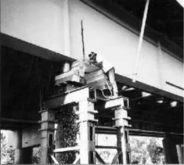
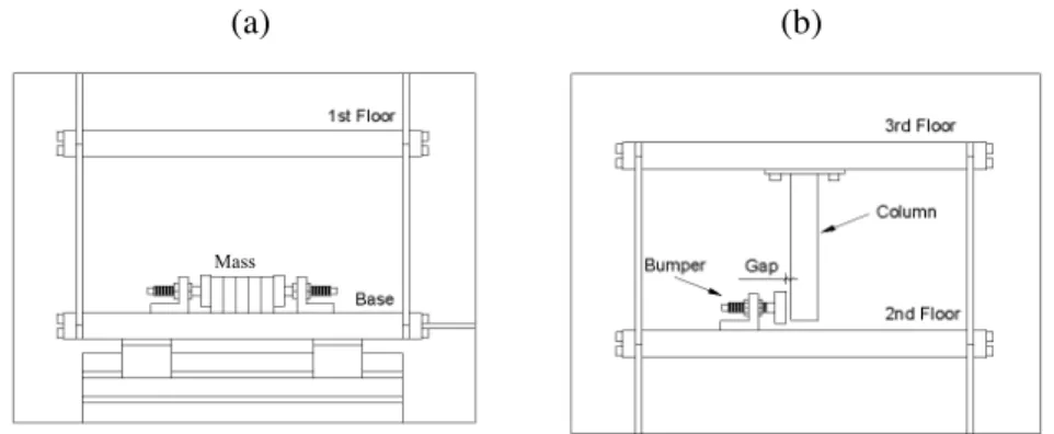
Figure 4.3. Structural details of the sources of simulated operational and environmental changes: (a) mass-loading added at the base; and (b) nonlinearity source. ...64

!

Figure 4.4. Shear-building model of the test structure. ...65

!

Figure 4.5. Numerical (NM) and experimental (Exp) mode shapes of the baseline condition: (a) second; (b) third; and (c) fourth mode shapes. ...66

!

(10)

vi

Figure 4.7. Responses from Channel 5 due to the measured experimental excitation at Channel 1 (State#1): (a) experimental time series; and (b) time series derived from the

numerical model... 67

!

Figure 4.8. ACFs of the experimental and numerical responses. ... 68

!

Figure 4.9. PSDs obtained from experimental and numerical time responses. ... 68

!

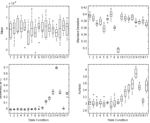
Figure 4.10. Box plots of the first four statistical moments of all 10 time series from Channel 5... 70

!

Figure 4.11. Box plots of the skewness and kurtosis of all 10 time series from Channel 1. ... 70

!

Figure 4.12. Box plots of the ACFs, for the first 15 coefficients, of all time series from Channel 5: (a) State#1; and (b) State#14... 70

!

Figure 4.13. PDFs estimated from acceleration time series from Channel 5 of two undamaged (State#1 and 7) and two damaged (State#14 and 17) states using a kernel density estimator... 72

!

Figure 4.14. Normal probability plots of four state conditions at Channel 5: (a) State#1; (b) State#7; (c) State#14; and (d) State#17... 73

!

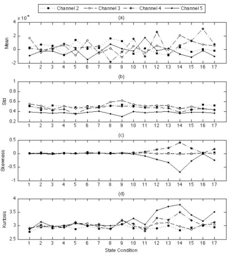
Figure 4.15. First four statistical moments based on one acceleration time series from Channel 2-5 of each state condition: (a) mean; (b) standard deviation; (c) skewness; and (d) kurtosis. ... 74

!

Figure 4.16. CMIF for one FRF from Channel 5 of State#1. ... 75

!

Figure 4.17. Curve fitting example on the FRFs from Channel 2-5 for the selected frequency range between 25-80 Hz (State#1)... 75

!

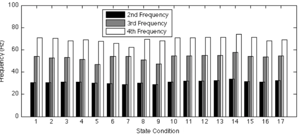
Figure 4.18. Natural frequencies estimated based on one test of each state condition... 77

!

Figure 4.19. Natural frequency deviations of all state conditions from the baseline condition (State#1). ... 77

!

Figure 4.20. AR order estimation based on one time series of Channel 5 from the baseline condition (State#1) using four different techniques: (a) AIC; (b) PAF; (c) RMS; and (d) SVD. ... 79

!

Figure 4.21. AIC functions estimated using time series from Channels 2-5. ... 79

!

Figure 4.22. Comparison of the measured and predicted time series from the baseline condition at Channel 5 using: (a) AR(5); (b) AR(15); and (c) AR(30) models. ... 80

!

Figure 4.23. Residual-error histograms along with the superimposed Gaussian distribution based on one time series from the baseline condition at Channel 5: (a) AR(5); (b) AR(15); and (c) AR(30) models... 81

!

(11)

vii Figure 4.24. Log PSDs of the residual errors based on one time series from the baseline condition

at Channel 5: (a) AR(5); (b) AR(15); and (c) AR(30) models. ...81

!

Figure 4.25. ACFs of one acceleration time series at Channel 5 from: (a) State#1; (b) State#7; (c)

State#14; and (d) State#17. ...82

!

Figure 4.26. ACFs of the residual errors at Channel 5 from State#1, 7, 14, and 17 using: (a)

AR(5); (b) AR(15); and (c) AR(30) models. ...83

!

Figure 4.27. Lag plots of the original time series from Channel 5: (a) State#1; (b) State#7; (c)

State#14; and (d) State#17. ...84

!

Figure 4.28. Lag plots of the AR(5) model residual errors from Channel 5: (a) State#1; (b)

State#7; (c) State#14; and (d) State#17. ...84

!

Figure 4.31. RMS of the residual errors using 8177- (original) and 2044-points (grouped). ...86

!

Figure 4.32. AR parameter amplitudes for all the 17 state conditions at Channel 5 using: (a)

AR(5); (b) AR(15); and (c) AR (30) models. ...87

!

Figure 4.33. Amplitude of the third parameter of all the state conditions at Channel 5 from the

three AR models. ...87

!

Figure 4.34. AR(15) parameters, in concatenated format, from one test (Channel 2-5) of each state

condition. ...88

!

Figure 4.35. STFT analysis of signal from State#1, Channel 4: (a) time-frequency-amplitude

representation; and (b) time-frequency representation. ...91

!

Figure 4.38. STFT analysis; individual spectrograms in concatenated format, Channel 4: (a)

time-frequency-amplitude representation; and (b) time-frequency representation...94

!

Figure 4.39. CWT of time series from State#1, Channel 4: (a) time-frequency-amplitude

!

Figure 4.40. CWT of time series from State#10, Channel 4: (a) time-frequency-amplitude

(12)

viii

Figure 4.42. Details of the WT coefficients based on time series from Channel 4 for: (a) State#1; and (b) State#14. ... 99

!

Figure 4.43. Detection of singularities: (a) original entire time series from Channel 4 of State#10;

and (b) AR(15) residual errors. ... 100

!

Figure 4.44. WT of the time series from State#10, Channel 4. ... 100

!

Figure 4.45. Singularities detection at Channel 4 using on time series from State#10: (a) portion of

the time series; (b) Holder exponent function; (c) AR(5) residual errors; (d) AR(15) residual errors; and (e) AR(30) residual errors. ... 101

!

Figure 4.46. Projection of the AR(5) parameters onto the first: (a) two; and (b) three principal

components. ... 102

!

components. ... 103

!

components. ... 103

!

Figure 4.49. Correlation coefficients between Channel 1 and Channel 1-5 (

!

r_1,1:5) along with correlation coefficients between Channel 5 and Channel 1-5 (

!

r_5,1:5)... 104

!

Figure 4.50. Correlation coefficients of pair of channels for all state conditions (State#1-17): (a)

Channel 5 and 1; (b) Channel 5 and 2; (c) Channel 5 and 3; and (d) Channel 5 and 4. . 104

!

Figure 4.51. Binary classification (undamaged and damaged conditions) using AR(15) parameters

from one time series of each state condition at Channel 5 (DataSet2007). ... 106

!

Figure 4.52. Cluster tree of the state conditions in Figure 4.51 (DataSet2007). ... 107

!

Figure 4.53. Binary classification (undamaged and damaged conditions) using AR(15) parameters

from one time series of each state condition at Channel 5 (DataSet2009). ... 107

!

Figure 4.54. Cluster tree of the state conditions in Figure 4.53 (DataSet2009). ... 108

!

Figure 4.55. The Shewhart X-Bar control charts of the mean of the grouped AR(15) residual

errors; outliers are represented by crosses. ... 110

!

Figure 4.56. Number of outliers falling outside the control limits defined based on data from the

baseline condition (State#1); the horizontal dashed line corresponds to the maximum number of outliers among the undamaged states (State#5). ... 111

!

Figure 4.57. Number of outliers falling outside the control limits defined based on data from all

(13)

ix maximum number of outliers among the undamaged states (State#5); in overlap

format one can see the log-scale version of the figure...111

!

Figure 4.58. Singular values obtained from the state-space reconstructions of the undamaged and

damaged structural state conditions at Channel 5, where the bold line represents the baseline condition (State#1)...113

!

Figure 4.59. AIC function of the MAR model for increasing order p=1,2,…,25 (Channel 5). ...114

!

Figure 4.60. Predicted trajectory of the baseline condition (black dots) along with the predicted

trajectories from test conditions (gray dots) at Channel 5 for m=3: (a) State#1; (b)

State#1 and 7; (c) State#1 and 10; and (d) State#1 and 14. ...115

!

Figure 4.61. Feature extraction at Channel 5 for m=3: (a) plot of

!

d2 from all state vectors from the undamaged (State#1-9) and damaged state conditions (State#10-17), in concatenated format, along with one-sided threshold (horizontal dashed line); and (b) number of outliers, or

!

d2 values beyond the threshold, along with the average sum-of-square MAR errors (

!

")...116

!

Figure 4.62. Relative distances between the undamaged and damaged conditions as a function of

the embedding dimension m; Dm is the distance between the mean of both d2

distributions; Dout is the distance between the minimum number of outliers among the damaged state conditions and the maximum number of outliers among the

undamaged state conditions. ...117

!

Figure 4.63. Outlier detection and feature extraction per structural condition in the four

accelerometers (Channel 2-5) for m=12; number of outliers along with the average sum-of-square MAR errors (

!

") in log scale. ...118

!

Figure 4.64. Number of outliers along with the average sum-of-square MAR(p) errors (

!

") in log scale per structural state condition: (a) based on a global embedding (Channel 2-5, M=12 and p=7); and (b) based on a semi-global embedding (Channel 4-5, M=12,

and p=8)...119

!

Figure 4.65. Average AIC function for four independent AR(p) models of increasing order p using

baseline-based time series (State#1) from the four accelerometers (Channel 2-5). ...120

!

Figure 4.66. ROC curves: (a) linear scale; and (b) log scale to highlight the differences between

curves. ...122

!

Figure 4.67. DIs calculated based on feature vectors from the undamaged (black) and damaged

(gray) state conditions along with thresholds defined by the 95% cut-off value over the training data: (a) AANN-; (b) FA-; (c) MSD-; and (d) SVD-based algorithms. ...124

!

(14)

x

of factors: (a) AANN-; and (b) FA-based algorithms... 125

!

Figure 4.69. Comparison of the behavior of the CIC as a function of model order using: (a)

4096-point; and (b) 1024-point time series. ... 127

!

Figure 4.70. Estimated PDF for each variable, or AR(15) parameter, of the original undamaged

feature vectors from Channel 5. ... 127

!

Figure 4.71. Four theoretical chi-square distributions,

!

"_m2, along with PDFs of the DIs from undamaged condition and assuming AR(p) models of increasing order p=m=5, 15, 30, and 50... 128

!

Figure 4.72. Correlation coefficients between the theoretical chi-square distributions,

!

"_m2, and PDFs of the DIs from the undamaged condition for increasing AR(p) model order

p=m=1,2,…,50. ... 128

!

Figure 4.73. ROC curves for AR(p) models of varying order p=5,10,…,50 at: (a) Channel 2; (b)

Channel 3; (c) Channel 4; and (d) Channel 5... 129

!

Figure 4.74. True-detection rate for fixed false-alarm rate equals to 0.1 at Channels 2-5. ... 130

!

Figure 4.75. Percentage of Type I and Type II errors for varying AR model order p=1,2,…,50

assuming a level of significance equals to 10%; (a) Channel 2; (b) Channel 3; (c)

Channel 4; and (d) Channel 5... 131

!

Figure 4.76. PDFs based on the DIs of all tests from undamaged and damaged conditions along

with a threshold (vertical dashed line) defined by the 90% confidence interval of the

!

"152 distribution when using AR(15) parameters as damage-sensitive features and

50% of the entire undamaged data sets to establish the normal condition... 132

!

Figure 5.1. Alamosa Canyon Bridge near to Truth or Consequences, New Mexico, USA, in 2008. 140

!

Figure 5.2. Schematic representation of the accelerometers and driving point (DP) locations... 141

!

Figure 5.3. Attachment of the accelerometers to the bridge: (a) on the bottom of the steel girders;

and (b) on the deck surface. ... 142

!

Figure 5.4. An impact being applied adjacent to the driving point (in 2008)... 143

!

Figure 5.5. Picture of the area underneath the first span with the data acquisition system (in

2008). ... 143

!

Figure 5.6. Response caused by a hammer impact (time08_3): (a) force; and (b) acceleration time

series at node 15. ... 145

!

Figure 5.7. FRFs in overlaid format (time08_3)... 145

!

Figure 5.8. Transverse cracking on the surface of the deck pavement (in 2008). ... 146

!

(15)

xi Figure 5.9. Variability in the modal parameters along with the differential temperature across the

deck during the 24-hour test in 1996: (a) first natural frequency; and (b) first damping ratio. ...148

!

Figure 5.10. Variability in the modal parameters along with the differential temperature across the

deck during the 24-hour test in 1997: (a) first natural frequency; and (b) first damping ratio. ...148

!

Figure 5.11. Modal parameters of all tests in 1996, 1997, and 2008: (a) natural frequencies; and

(b) damping ratios. ...150

!

Figure 5.12. First mode shape for the maximum and minimum natural frequencies observed in: (a)

!

Figure 5.13. SDOF system. ...152

!

Figure 5.14. Free vibration responses caused by two impulse forces (

!

I₁_and

!

I₂= I1" 2)...153

!

Figure 5.15. AR model analysis: (a) estimated parameters based on responses caused by

!

I₁ and

!

I₂_{; and (b) responses estimated using parameters from the response caused by}

!

I₁...153

!

Figure 5.16. Normalized 13-average AIC, RMS, SVD, and PAF functions during the 24-hour test

in 1996 (node 15). ...154

!

Figure 5.17. Normalized 11-average AIC, RMS, SVD, and PAF functions during the 24-hour test

in 1997 (node 15). ...154

!

Figure 5.18. Normalized 20-average AIC, RMS, SVD, and PAF of the tests performed in 2008

(node 15). ...155

!

Figure 5.19. Error bar (two standard deviations) with AR(25) parameters estimated at node 15

during the 24-hour test in 1996 along with the outlier-free means (dots). ...156

!

during the 24-hour test in 1997 along with the outlier-free means (dots). ...156

!

during the tests in 2008 along with the outlier-free means (dots). ...156

!

Figure 5.22. Outlier-free means of the AR parameters estimated in 1996, 1997, and 2008. ...157

!

Figure 5.23. Force time series for linearity check using tests performed in 2008: (a) low force

level, time08_1; and (b) high force level, time08_2...158

!

Figure 5.24. Average of the AR(25) parameters for linearity check using time08_1 and time08_2

tests performed in 2008 at node 15. ...158

!

Figure 5.25. Measured and predicted acceleration time series at 17:52 (1996) using an AR(25)

model with the 24-hour-average parameters of 1996: (a) full time series; and (b)

(16)

xii

windowed time series... 159

!

Figure 5.27. Measured and predicted acceleration time series at 17:20 (2008) using an AR(25)

model with the 24-hour-average parameters of 1996: (a) full time series; and (b)

windowed time series... 160

!

Figure 5.28. RMS of the AR(25) residual errors from the tests performed in 1996, 1997, and 2008. 160

!

Figure 5.29. RMS of the AR(25)-ARX(15,10) residual errors from the tests performed in 1996,

1997, and 2008. ... 161

!

Figure 5.30. RMS of the AR(25) residual errors from the tests performed in 1996, 1997, and 2008;

horizontal dashed line corresponds to the maximum value of 1997... 162

!

Figure 5.31. RMS of the AR(25)-ARX(15,10) residual errors from the tests performed in 1996,

1997, and 2008; horizontal dashed line corresponds to the maximum value of 1997. ... 162

!

Figure 5.32. Differential temperature across the deck along with the RMS of the AR(25) residuals,

with parameters estimated at 21:10, for each test at node 15 during the 24-hour test in 1996... 163

!

Figure 5.33. Differential temperature across the deck along with the RMS of the AR(25) residual

errors, with parameters estimated at 22:00, for the 24-hour tests in 1997 at node 15. ... 163

!

Figure 5.34. Averaged singular spectra at node 15 in 1996, 1997, and 2008... 164

!

Figure 5.35. Outlier detection of feature vectors composed of natural frequencies using the

MSD-based algorithm; threshold defined MSD-based on 99% confidence interval of a

!

"6

2_{. ... 166}

_!

SVD-based algorithm; threshold equals to 99% cut-off value over the DIs from the training data. ... 166

!

AANN-based algorithm; threshold equals to 99% cut-off value over the DIs from the training data assuming: (a) one factor; and (b) two factors. ... 167

!

FA-based algorithm; threshold equals to 99% cut-off value over the DIs from the training data assuming: (a) one factor; and (b) two factors. ... 167

!

Figure 5.39. Outlier detection of feature vectors composed of AR(25) parameters using the

MSD-based algorithm; threshold defined MSD-based on 99% confidence interval of a

!

"25

(17)

xiii Figure 5.40. Outlier detection of feature vectors composed of AR(25) parameters using the

SVD-based algorithm; threshold equals to 99% cut-off value over the DIs from the training data...169

!

AANN-based algorithm; threshold equals to 99% cut-off value over the DIs from the training data assuming: (a) one factor; and (b) two factors. ...169

!

FA-based algorithm; threshold equals to 99% cut-off value over the DIs from the training data assuming: (a) one factor; and (b) two factors...170

!

Figure 5.43. Estimated PDF of the DIs from the training data along with the theoretical

!

"252, when using the MSD-based algorithm. ...170

!

(18)

(19)

xv

LIST OF TABLES

Table 3.1. Accuracy of binary classification. ...53

!

Table 3.2. Feature extraction techniques along with potential detectable type of damages. ...55

!

Table 4.1. Data labels of the 17 structural state conditions...62

!

Table 4.2. Experimental along with numerical natural frequencies and damping ratios for State#1 (baseline contidion)...66

!

Table 4.3. Experimental natural frequencies and damping ratios of all state conditions. ...76

!

Table 4.4. Number and percentage of Type I and Type II errors for each algorithm. ...124

!

Table 4.5. Number of Type I and Type II errors. ...133

!

Table 5.1. Summary description of the data sets from the 24-hour test in July/August, 1996. ...144

!

Table 5.2. Summary description of the data sets from the 24-hour test in July, 1997. ...144

!

Table 5.3. Summary description of the data sets measured in September, 2008. ...145

!

Table 5.4. Daily average temperature and humidity records at Truth or Consequences, New Mexico. ...146

!

Table 5.5. Maximum and minimum values of the first natural frequency and damping ratio observed in 1996, 1997, and 2008. ...149

!

Table 5.6. Values of the first natural frequency and damping ratio observed in 1996, 1997, and 2008 at 10:00 (morning) and 17:20 (afternoon). ...149

!

(20)

(21)

xvii

NOTATION

All symbols used in this dissertation are defined when they first appear in the text. For the reader’s convenience, this section contains only the principal meanings of the commonly used acronyms and symbols. Some symbols denote more than one meaning, but their meaning should be clear when read in context.

Abbreviations

AANN Auto-associative neural network ACF Auto-correlation function AIC Akaike information criterion AR(p) Auto-regressive model of order p

ARX(a,b) Auto-regressive model with exogenous inputs (a auto-regressive and b exogenous input terms)

BMS Bridge management system CIC Consistent information criterion CMIF Complex mode indicator function COMAC Co-ordinate modal assurance criterion CWT Continuous wavelet transform

DI Damage indicator

FA Factor analysis

FHWA Federal Highway Administration FRF Frequency response function MAC Modal assurance criterion

MAR(p) Multivariate auto-regressive model of order p MSD Mahalanobis squared distance

NBI National Bridge Inventory

NBIS National Bridge Inspection Standards NDT Non-destructive testing

NI National Instruments

NTSB National Transportation Safety Board PAF Partial auto-correlation function PCA Principal components analysis PDF Probability density function PSD Power spectral density RFP Rational-fraction polynomial

(22)

xviii

SHM Structural health monitoring SPC Statistical process control SPR Statistical pattern recognition STFT Short-time Fourier transform SVD Singular value decomposition USA United States of America

WT Wavelet transform

Roman Symbols

!

d2 _{Mahalanobis squared distance}

!

e Residual error value

!

e Vector of residual errors

!

E

_{[ ]}

Expectation operator

!

E Matrix of residual vectors

! D Damping matrix ! i_, ! j_{, and} ! k Indices ! K Stiffness matrix !

m Feature vector dimension or embedding dimension

!

n Number of feature vectors

!

N Time series size or number of observations

!

N_t Total number of observations used in fitting auto-regressive models

!

M State matrix

!

p Number of regressive model parameters (or model order)

!

r_xz Correlation coefficient between

! x_and ! z ! R_xx Auto-correlation function of ! x !

R_xz Cross-correlation function between

! x and ! z !

s Response time series

!

t Time variable

!

v Response time series

! x Variable ! x Sample average of ! x !

x Feature vector (or vector of variables)

!

(23)

xix ! z Variable ! z Sample average of ! z !

z Feature vector (or vector of variables)

!

Z Matrix of feature vectors from the test data

Greek Symbols

!

" Level of significance

!

" Vector of exogenous parameters

!

" Sum-of-square of errors

!

" Matrix of factor loadings

!

µ Population mean

!

" Covariance matrix

!

" Population standard deviation

! "2 Population variance ! " Time lag !

" Vector of auto-regressive parameters (or mode shape vector)

!

" Matrix of mode shapes

!

"m2 Central chi-square distribution with

!

(24)

(25)

xxi

ABSTRACT

Damage Identification in Civil Engineering Infrastructure under Operational and Environmental Conditions

by Elói Figueiredo

Doctor of Philosophy in Civil Engineering Faculty of Engineering of the University of Porto, 2010

Joaquim A. Figueiras1_{and Charles R. Farrar}2

Real-world structures are subjected to operational and environmental condition changes that impose difficulties for detecting and identifying structural damage. In fact, the author believes that separating changes in sensor readings caused by damage from those caused by changing operational and environmental conditions is one of the biggest challenges for transitioning structural health monitoring (SHM) technology from research to practice. The SHM process is posed in the context of the statistical pattern recognition (SPR) paradigm, where vibration-based methods are applied to detect damage in civil infrastructure. Even though this paradigm intends to pave the way for data-based models applicable to systems of arbitrary complexity, the bridge structures are the focus of this dissertation.

The objective of this dissertation is to review, develop, and apply several SHM statistical procedures for feature extraction and statistical modeling for feature classification capable of detect damage on structures under unmeasured operational and environmental variations. In the feature extraction step, the auto-regressive (AR) model is focus of special attention due to its simplicity of application and capability to detect damage. Additionally, a novel algorithm for feature extraction is presented that uses the state-space reconstruction to infer the geometrical structure of a deterministic dynamical system from observed time series of a system response at multiple locations. The unique contribution of this algorithm is that it uses a multivariate auto-regressive model of a baseline condition to predict the state space, where the model encodes the embedding vectors rather than scalar time series. Moreover, four machine learning algorithms are presented to remove the effects of operational and environmental variations on the extracted features. These algorithms are desirable because they develop a functional relationship that models how changing operational and environmental conditions

1_{Full Professor, Faculty of Engineering of the University of Porto, Portugal}

(26)

xxii

The applicability of the SHM-SPR, along with the reviewed and proposed statistical procedures, is first demonstrated in a base-excited three-story frame structure tested in laboratory environment to obtain standard data sets from an array of sensors under several structural state conditions. Tests were performed with varying stiffness and mass conditions with the assumption that these sources of variability are representative of changing operational and environmental conditions (e.g. changing mass might represent varying live loads and changing temperature will influence stiffness properties on a structure). Damage is simulated through nonlinear effects introduced by a bumper mechanism that induces a repetitive, impact-type nonlinearity. This mechanism intends to simulate, for instance, the cracks that open and close under dynamic loads or loose connections that rattle.

Finally, the applicability of the SHM-SPR paradigm is demonstrated in 12-year span data from the real-world undamaged Alamosa Canyon Bridge, near to Truth or Consequences, New Mexico. Herein, the AR models and machine learning algorithms are focus of special attention. The former because their applicability on civil infrastructure is still limited, and the latter because they might be useful for real-world applications, in situations where the operational and environmental variations cannot be measured.

(27)

xxiii

RESUMO

Identificação de Dano em Infra-estruturas de Engenharia Civil sob Condições Operacionais e Ambientais

por Elói Figueiredo

Doutoramento em Engenharia Civil Joaquim A. Figueiras3 e Charles R. Farrar4

As estruturas estão sujeitas a alterações operacionais e ambientais que impõem dificuldades na detecção de danos estruturais. De facto, o autor acredita que, a separação das alterações nas respostas estruturais causadas por danos das alterações causadas por variações de natureza operacional e ambiental é um dos maiores desafios para a transição da monitorização da integridade estrutural (SHM) da investigação para a prática. Assim, o processo de SHM é integrado no contexto do paradigma de reconhecimento de padrões (SPR), onde métodos estatísticos baseados em vibração estrutural são aplicados para detecção de danos em infra-estruturas de engenharia civil. Mesmo embora o paradigma tem como objectivo abrir caminho a métodos estatísticos aplicáveis a sistemas de complexidade arbitrária, as pontes serão alvo de especial atenção nesta dissertação.

O objectivo desta dissertação é o de rever, desenvolver e aplicar vários métodos estatísticos para a extracção de características (ou parâmetros da resposta estrutural) e para classificação das mesmas no contexto do paradigma SHM-SPR, capaz de detectar danos em estruturas sob condições operacionais e ambientais variáveis. Na fase de extracção de características é dado ênfase ao modelo auto-regressivo devido à sua capacidade e simplicidade de aplicação. Além disso, um novo algoritmo baseado no conceito de state-space reconstruction é proposto para inferir a estrutura geométrica de um sistema dinâmico e determinístico observado através de respostas estruturais em forma de séries temporais. A contribuição original deste algoritmo reside na utilização de um modelo auto-regressivo multi-variável do estado inicial, onde o modelo incorpora vectores ao invés de escalares. Uma hipótese é testada em que o modelo multi-variável não consegue prever o estado inicial quando o dano está presente. Além disso, quatro algoritmos de aprendizagem são apresentados para remover os efeitos das variações operacionais e ambientais sobre os dados de respostas estruturais. Esses algoritmos são desejáveis porque eles desenvolvem uma relação funcional entre as variações operacionais e ambientais e a distribuição das características.

3_{Professor Catedrático, Faculdade de Engenharia da Universidade do Porto, Portugal}

(28)

xxiv

respostas estruturais através da simulação de diversas condições operacionais e ambientais e também de dano. Testes foram realizados com diferentes condições de rigidez e de massa, com o pressuposto de que estas fontes de variabilidade são representativas da evolução das condições operacionais e ambientais (por exemplo, alteração da massa simula acções variáveis e a mudança de temperatura pode influenciar propriedades de rigidez de uma estrutura). O dano é simulado através de efeitos não lineares introduzidos por um mecanismo constituído por uma coluna suspensa e por um batente. Este mecanismo tem como objectivo simular, por exemplo, fendas que abrem e fecham devido a acções dinâmicas ou ligações aparafusadas soltas.

Finalmente, a aplicabilidade do paradigma SHM-SPR é testada em respostas estruturais, de três períodos distintos dentro de um intervalo de 12 anos, recolhidas de um vão da ponte Alamosa Canyon Bridge, perto de Truth or Consequences, Novo México, Estados Unidos da América. Os modelos auto-regressivos e os algoritmos de aprendizagem são foco de atenção especial. Os primeiros porque a sua aplicabilidade em pontes é ainda limitada e os últimos porque eles são úteis em aplicações reais, onde as variações operacionais e ambientais não podem ser medidas.

(29)

xxv

ACKNOWLEDGEMENTS

I would like to give special thanks to my advisors, Joaquim Figueiras and Chuck Farrar. Their constant support, advice, and commitment to my research have been invaluable. I would like to thank Gyuhae Park for his one-to-one guidance that gave me while working at Los Alamos National Laboratory (LANL) and Mike Todd as my host while working at the University of California, San Diego (UCSD). Also, a special thanks to Keith Worden from the University of Sheffield for his collaboration and lessons.

Thanks to my friends and collaborators at LANL/UCSD including Stuart Taylor, Eric Flynn, Kevin Farinholt, David Mascarenas, Greg Jarmer, Samory Kpotufe, Eric Moro, and Dustin Harvey. Also, a special thanks to Kathie Womack on behalf of the technical staff members at LANL.

Thanks to my friends and collaborators at Faculty of Engineering of the University of Porto including José Santos, Lino Maia, and Américo Dimande.

A special thanks to my forever professors and friends Luís Juvandes, Arlindo Begonha, Ana Maria Sarmento, and Rui Carneiro Barros.

I would like to acknowledge support through the four-year PhD Fellowship SFRH/BD/29460/2006 given by the Fundação para a Ciencia e a Technologia (FCT). Also, I would like to acknowledge support through the UCSD Jacobs School of Engineering Fellowship for the six-month period of studies at that institution and Fundação Luso-Americana (FLAD) for the institutional research grant number 036/2009 to reinforce the capacity of action of research collaboration on SHM between the Engineering Institute and the Laboratory for the Concrete Technology and Structural Behaviour. Lastly but most importantly, I would like to thank my family and Rute for their constant support throughout the entire PhD program, especially for their comprehension during my period of studies in the USA.

(30)

(31)

1. INTRODUCTION

1.1 SHM Background

The process of implementing a damage detection strategy for aerospace, civil, and mechanical infrastructure is referred to as structural health monitoring (SHM). Here damage is defined as changes to the material and/or geometric properties of these systems, including changes to the boundary conditions and system connectivity, which adversely affect the system’s current or future performance. The goal of SHM is to improve the safety and reliability of aerospace, civil, and mechanical infrastructure by detecting damage before it reaches a critical state. To achieve this goal, technology is being developed to replace qualitative visual inspection and time-based maintenance procedures with more quantifiable and automated damage assessment processes. These processes are implemented using both hardware and software with the intent of achieving more cost-effective condition-based maintenance. A more detailed discussion on SHM can be found in [1, 2]. Nevertheless, throughout this chapter, a general overview of the SHM for civil infrastructure, with special emphasis on bridges, will be presented.

1.1.1 Historical Perspective

The damage detection in the past was mainly performed based on visual inspection methods, with occasional application of conventional non-destructive testing (NDT) techniques such ultrasonic and acoustic emission (e.g. tap tests on train wheels). However, vibration-based damage detection methods have received considerable attention during the last 40 years. A brief review of the SHM historical evolution using vibration-based structural damage identification is given below. However, the author recommends Doebling et al. [3] and Sohn et al. [4] for a review of literature on this subject.

The most successful application of damage detection using vibration-based methods has been reported for rotating machinery. The shorter lifetime, controlled operational and environmental variability along with well-defined damage types permitted one to build up large data sets, from both undamaged and damaged conditions, and to pave the way for application of pattern recognition algorithms. In the broad sense, a pattern recognition algorithm simply assigns estimated spectra to types of damage. A relative recent state of the art review on monitoring rotating machinery was made by Randall [5, 6].

Damage identification in civil engineering infrastructure under operational and environmental conditions

FACULTY OF ENGINEERING

OF THE

UNIVERSITY OF PORTO