Instrumentation and signal processing applied to atmospheric electricity

(1)

UNIVERSIDADE DE ÉVORA

ESCOLA CIÊNCIAS E TECNOLOGIAS

DEPARTAMENTO DE FÍSICA

Instrumentation and signal processing applied to

Atmospheric Electricity

Ricardo Filipe Carrão da Conceição

Orientação:

Orientador:

Professor Doutor Mouhaydine Tlemçani

Coorientador:

Doutor Hugo Manuel Gonçalves da Silva

Mestrado em Engenharia Mecatrónica

Dissertação Évora, 2015

(2)

UNIVERSIDADE DE ÉVORA

ESCOLA CIÊNCIAS E TECNOLOGIAS

DEPARTAMENTO DE FÍSICA

Instrumentation and signal processing applied to

Atmospheric Electricity

Ricardo Filipe Carrão da Conceição

Orientação:

Orientador:

Professor Doutor Mouhaydine Tlemçani

Coorientador:

Doutor Hugo Manuel Gonçalves da Silva

Mestrado em Engenharia Mecatrónica

Dissertação Évora, 2015

(3)

Resumo

Intrumentação e processamento de

sinal aplicado à Electricidade Atmosférica

O conhecimento atual diz-nos que a atmosfera da Terra em si aprensenta-se como um circuito elétrico global, que proporciona uma atmosfera continuamente eletrificada. O estudo deste circuito global, bem como os efeitos, globais e locais, sobre a componente vertical do campo eléctrico atmosférico, geralmente designada como gradiente de potencial, são de grande importância não só devido à resposta dinâmica do gradiente de potencial em relação a estes efeitos, mas também porque é possível recuperar informações a partir das suas medidas para inferir propriedades importantes de fatores externos. Desta forma, o impacto dos efeitos externos sobre o gradiente de potencial foram estudados para Lisboa desde 1955 a 1991. As medições foram feitas usando um electrómetro Benndorf na estação meteorológica de Portela (nos subúrbios de Lisboa e perto do Aeroporto de Lisboa). Como Lisboa é uma cidade histórica, muito povoada e perto do mar, que fornece um conjunto de efeitos externos, como a poluição, que podem e devem ser estudados com recurso a mediadas de gradiente de potencial. O estudo elaborado contempla o efeito da poluição antropogénica como um efeito local no gradiente de potencial e a confirmação de um ciclo semanal persistente, devido à poluição urbana. Este estudo foi complementado com uma análise da dependência da direção do vento. Um segundo estudo foi feito sobre o efeito da humidade relativa sobre o gradiente de potencial. Uma formulação foi desenvolvida para relacionar propriedades microfísicas dos aerossóis, principalmente o parâmetro de higroscospicidade, com a medida macrofísica que é o gradiente de potencial. Resultados razoáveis foram obtidos entre o modelo e os dados experimentais, indicando a presença de uma fracção de aerossóis higroscópicos. Um terceiro estudo foi baseado num evento particular, o incêndio do Chiado, que teve lugar no dia 25 de agosto de 1986 e é considerado o acidente mais trágico que ocorreu em Lisboa desde o terramoto de 1755. O efeito da pluma de fumo sobre o gradiente de potencial, assim como o transporte da pluma desde área do Chiado até à Portela foram estudados. Foi observado pela primeira vez que o fumo do incêndio foi responsável por um

(4)

aumento de gradiente de potencial significativo com uma baixa probabilidade de ocorrer por acaso. Este estudo pode incentivar o uso de medições gradiente de potencial em detectores de rede de incêndios. Finalmente, foram realizadas simulações sobre o Circuito Global Elétrico (circuito primário) e seu acoplamento para medições locais (circuito secundário). O objectivo foi o de separar os efeitos globais dos efeitos locais gerados pela poluição sobre a resistência colunar na superfície da Terra onde as medições são realizadas.

(5)

Abstract

Present knowledge tells us that Earth’s atmosphere itself represents a global electrical circuit, which provides a continuous electrified atmosphere. The study of this global circuit as well as the effects, globally and locally wise, on the vertical component of the atmospheric electrical field, usually referred as Potential Gradient, are of great importance not only because of the dynamical response of the Potential Gradient to those effects, but also because it is possible to retrieve information from its measurements to infer the proprieties of important external factors. In this way, the impact of external effects on the Potential Gradient was studied for Lisbon from 1955 to 1991. The measurements were done using a Benndorf Electrograph at the Portela meteorological station (in the suburbs of Lisbon and near the Lisbon Airport). Since Lisbon is an historical city, very populated and near sea, it provides a set of external effects, like pollution, which can and should be studied through measurements of Potential Gradient. The core study done contemplates the effect of anthropogenic pollution as a local effect on the Potential Gradient and the confirmation of a persistent weekly cycle, due to urban pollution. This study was complemented with a wind direction dependence analysis. A second study was made regarding the effect of relative humidity on the Potential Gradient. A formulation was developed to relate microphysical proprieties of the aerosols, mainly the hygroscopicity parameter, with the macrophysical measure of Potential Gradient. Reasonable fits were obtained between the model and the experimental data indicating the presence of a small fraction of hygroscopic aerosols. A third study was based on a particularly event, the Chiado’s fire that took place on 25th_{of August} 1989 and is considered the most significant hazard which occurred in Lisbon since the 1755 earthquake. The effect of the smoke plume on the Potential Gradient, but also how the plume travelled from the Chiado area to Portela was studied. It was observed (for the first time) that the fire smoke was responsible for a significant Potential Gradient increase with a low probability to occur by chance. This study might encourage the use of Potential Gradient measurements in fire network detectors. Finally, simulations regarding the Global Electrical Circuit (primary circuit) and its coupling to local measurements (secondary circuit) were performed. The objective was to separate the global effects from the local effects generated by pollution on the columnar resistance at Earth surface where measurements are made.

(6)

“I have no special talents. I am only passionately curious”

(7)

I dedicate this dissertation especially to my mother Maria, my sister Vera, my nephew Francisco, my niece Carminho, my grandmothers Angelica and Clotilde, my grandfather

(8)

Acknowledgments

Firstly, I would like to thank to my supervisor, Mouhaydine Tlemçani, for his effort in the development of this dissertation and for his humor and ideas given through the all process. Secondly I would like to mention the help of my co-supervisor, Hugo Gonçalves Silva, since he was the main pillar of this dissertation, not only because of his academic experience, namely from a scientific point of view, but also for his guidance, leading me always in the right path.

I am also grateful to Professor Giles Harrison and Keri Nicoll for their massive knowledge and help through the scientific articles, which compose this dissertation. Besides the fact that they are two of the major figures on atmospheric electrical field in the world for quite some time they were also very helpful. Having the chance to work with these figures was quite an honor for me and I feel privileged.

I want to express my thanks to Professor Heitor Reis for his support on article revision and for his thoughts, which contributed greatly for the evolution of this dissertation and my academic experience.

Marta Melgão and Samuel Bárias for their disposition of helping me understating how to assemble an electrical field measurement system, which we tested in Beja air force base and Évora.

I am grateful to James Matthews and Matthew Wright from University of Bristol and Sergio Pereira for his experience in the aerosols field and for their help in aerosol hygroscopic growth matter.

(9)

Paula Brás Mendes for her help in Lisbon’s climatology, Claudia Serrano for data digitalization and Dr. Mário Figueira, from the former Institute of Meteorology, for installing the Potential Gradient sensor and make such measurements.

Bruno Besser from Graz University for his effort in providing information about Benndorf Electrometer.

My family and my girlfriend offered a support pillar through which I could maintain myself confident and keep up my moral through the adversities found along this dissertation. They kept my motivation always high and helped me to understand how obstacles can be overcome and how to learn from them.

Finally, I would like to acknowledge the support of the Portuguese Foundation for Science and Technology (Fundação para Ciência e Tecnologia, FCT) through the 1 year research grant from a FCT/COMPETE project EAC: FCOMP-01-0124-FEDER-029197 PTDC/GEO-FIQ/4178/2012; which Hugo G. Silva is responsible for and that allowed me to fulfill the objectives outlined for the present work.

(10)

List of Figures

Figure 1.1 Benjamin’s Franklin portrait by Joseph Siffred Duplessis (http://www.nPG.si.edu). ... 2 Figure 1.2 Benjamin’s experiment proposal to check cloud electrification, (Experiments and Observations on Electricity, Made at Philadelphia in America). ... 2 Figure 1.3 Apparatus used by T.F.Dalibard for Benjamin’s experience. (Franklin, Expériences et Observations sur Électricité…, 2nd ed., vol.2, pag. 128, an extended translation from English by T.F.Dalibard). ... 3 Figure 1.4 Pierre-Charles Le Monnier portrait by Nicolas-Bernard Lépicié (http://fr.wikipedia.org). ... 4 Figure 1.5 Giovanni Battista Beccaria portrait by Franz Joseph Anton von Thun-Hohenstein (http://www.gettyimages.pt). ... 5 Figure 1.6 Horace Bénédict de Saussure portrait by Jean Pierre Saint-Ours (http://www.summitpost.org). ... 5 Figure 1.7 Lord Kelvin portrait by Elizabeth King (http://www.docbrown.info). ... 6 Figure 1.8 Photographically recorded PG at Kew Observatory in 1861 (Aplin and Harrison, 2013). ... 7 Figure 1.9 a) J. J. Thompson portrait by George Fiddes Watt (http://www.bbc.co.uk); b) Wilhelm Conrad Roentgen (http://www.nobelprize.org). ... 7 Figure 1.10 C.T.R Wilson portrait by James Gunn (http://www.sid.cam.ac.uk). ... 8 Figure 1.11 Carnegie vessel photograph courtesy of Carnegie Institution of Washington. . 8 Figure 1.12 Carnegie and Maud hourly averaged PG in % of mean (Whipple and Scrase, 1936). ... 9 Figure 1.13 Active Thunder area around the world (Whipple and Scrase, 1936). ... 9 Figure 1.14 Processes of interest in the global electric circuit. Charge separation in thunderstorms, which occur in disturbed weather regions, creates a substantial potential difference between the highly conducting regions of the ionosphere and the Earth’s surface. The positive potential of the ionosphere (positive with respect to the Earth’s surface) is

(14)

distributed to fair-weather and semi-fair-weather regions, where a small current (whose density is JC) flows vertically. When this current flows through clouds it generates charge near the upper and lower cloud edges, which can influence cloud microphysical processes. (In this diagram, Mesospheric Convective Systems, which are large scale thunderstorms late in their evolution and which favor sprite generation above them, are indicated by MCS; sprites are one example of Transient Luminous Events (TLEs); Cloud Condensation Nuclei

are shown as CCN). ... 13

Figure 1.15 Conductivity profile. ... 17

Figure 1.16 Schematic representation of small ion clusters formations. ... 18

Figure 2.1 Schematic of water dropper equaliser (Gendle, 1912). ... 23

Figure 2.2 Lord’s Kelvin Electrometer schematic (www.orau.org). ... 24

Figure 2.3 Benndorf’s Electrometer from http://physik.uibk.ac.at. ... 25

Figure 2.4 Benndorf’s Electrometer schematic (Klemens R., 2003). ... 25

Figure 2.5 Field mill operating principle (http://www.missioninstruments.com). ... 27

Figure 2.6 JCI 131/F internal design. ... 28

Figure 2.7 Photograph ADC-212. ... 29

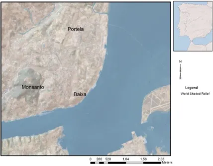
Figure 3.1 Left figure, geomorphology of Lisbon region with three main features marked: Serra de Monsanto, Baixa (city center), and Portela Airport (location of the PG sensor). Right figure, the rectangle marks the geographical location of Lisbon in Portugal ... 37

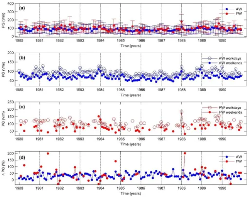
Figure 3.2 Mean monthly values of PG measured from Portela during the period from 1980 until 1990: a) PG for AW and FW (error bars represent standard deviations); b) AW week and weekends PG; c) FW week and weekends PG; d) AW and FW-PG relative difference between workdays and weekends, ΔPG. ... 41

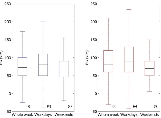
Figure 3.3 Boxplot of hourly PG values for AW (blue): a) whole week, b) workdays, and c) weekend; boxplot for FW (red): d) whole week, f) workdays, and g) weekends. A black line in all boxes marks median and the outliers are not presented. ... 42

Figure 3.4 Annual behavior of: a) PG for AW and FW; (b) ΔPG for AW and FW. Error bars represent standard deviations. ... 44

(15)

Figure 3.5 Annual averages from 1980 until 1990: a) PG for AW and FW; ΔPG for AW and FW. Error bars represent standard deviations. ... 45 Figure 3.6 Lomb-Scargle periodograms calculated using the LSP implementation in MATLAB (Brett, 2001) for 1980-1990: a) AW; b) FW. The following parameters were used hifac=1 (that defines the frequency limit as hifac times the average Nyquist frequency), ofac=4 (oversampling factor). ... 46 Figure 3.7 Color surface plot of Lomb-Scargle periodograms for each year: a) AW; b) FW. ... 47 Figure 3.8 Noise Upper panel: Evolution of the n-exponent from the Lomb-Scargle periodograms shown in Figure 3.6 and Figure 3.7 along the years for period below Tc = 2 days (empty circle) and above 2 days (full circle): a) AW; b) FW. ... 48 Figure 4.1 Location of the Portela meteorological station (yellow pin) and the industrial region of Setubal (red pin) are marked. The Atlantic Ocean and Iberian Peninsula are also indicated. A wind rose measured at Portela is also shown. ... 56 Figure 4.2 Distributions of the hourly PG values, in logarithmic scale, for the four wind sectors: NW, NE, SE, and SW. ... 58 Figure 4.3 Daily behavior of hourly PG values in a boxplot representation. The four wind sectors are considered: NW, NE, SE, and SW. ... 59 Figure 4.4 𝑅𝐻 dependence of daily averaged PG values of all sectors: NW, NE, SE, and SW. Bins with Δ𝑅𝐻 = 5 % in the 𝑅𝐻 range from 30 % to 100 % were used. The label attributed to a bin corresponds to its upper limit. Vertical lines mark the hygroscopic growth region, in which the analysis is focused. ... 60 Figure 4.5 Fits of the model to the wind sectors: a) NW; b) NE, The error bars represent the median absolute deviation (MAD), the solid-line the fitted curve and the dashed-lines the model function but with a variation in  of 40 % above and bellow the fitted valued. ... 62 Figure 4.6 Boxplots of the four wind sectors: a) NW, b) NE, c) SW and d) SE, divided in workdays (WD) and weekends (WK). ... 66 Figure 4.7 Daily behavior of the median PG values for 1980 to 1990 separated in workdays (WD) and weekends (WK) for each wind sector: a) NW, b) NE, c) SW and d) SE. ... 67

(16)

Figure 4.8 Lomb-Scargle Spectra corresponding to the four wind sectors. The following parameters were used hifac=1 (that defines the frequency limit as hifac times the average Nyquist frequency), ofac=4 (oversampling factor). ... 68 Figure 5.1 Image of the Chiado’s fire that took place at Lisbon city center; courtesy of the Municipal Archive of Lisbon. ... 70 Figure 5.2 PG data measured at Portela during 1988 (the green line denotes the PG peak of Chiado’s fire on 26th_{August). ... 72} Figure 5.3 a) distribution of PG values for all the year of 1988; b) distribution of PG values for the summer of 1988. The arrows point to the anomalous PG value in study. ... 73 Figure 5.4 Hourly mean behavior of the PG at Portela calculated from all year of 1988 (black curve), PG during 25th (red curve) and 26th of August 1988 (blue curve). ... 75 Figure 5.5 Meteorological conditions from 25th and 26th of August 1988 for Portela meteorological station (Lisbon airport): a) Potential Gradient; b) Visibility; c) Wind Speed; d) Wind Direction; e) Relative Humidity (𝑅𝐻). The vertical lines denote the start of the fire (first green line) and the PG peak hour (second green line). The horizontal red dash line in c) marks the fair-weather limit for wind speed, 6 m/s, according to Voeikov (1965). The black arrow in d) marks the moment when the smoke plume started travelling to Portela. 78 Figure 5.6 Rose wind representation in Portela during 1988 (a 3D perspective is used). The white arrow marks wind rotation in time from 25th of August at 07:00 up to 26th of August at 18:00 (UTC). These moments are marked in the figure. The wind speed varies according to 4 colors increasing its magnitude from light blue, dark blue, green and yellow. The increasing radius represents an increase in the observations. The Chiado’s fire is marked with red pin and Portela station marked with a yellow one... 79 Figure 5.7 Forward trajectories calculated using Hysplit-4 for air masses at 750 m starting at 05:00 h 25th August (first white trajectory) with a new trajectory created each 5 hours (blue trajectories) until 16:00 h 26th August (last black trajectory). The Chiado’s fire is marked with red pin and Portela station marked with a yellow one. NOAA Air Resources Laboratory. ... 81 Figure 5.8 Model projections of the plume spread from Chiado’s fire: a) 25th August, 17:00 h; b) 26th August, 07:00 h; c) 26th August, 18:30 h; The smoke particle concentration varies

(17)

according to 4 colors increasing its magnitude from light blue, to dark blue, green and yellow. The Chiado’s fire is marked with red pin and Portela station marked with a yellow one. NOAA Air Resources Laboratory. ... 82 Figure 6.1 Diagram of the circuit model. ... 86

Figure 6.2 a) PG values simulated with the first set of parameters; b) Ionosphere Potential derived from the thunderstorms voltage source and resistance for the first set of parameters; c) PG values simulated with the second set of parameters; d) Ionosphere Potential derived from the thunderstorms voltage source and resistance for the second set of parameters. ... 88

(18)

List of Tables

Table 3.1 Mean, median, standard deviation, skewness, kurtosis, and number of hours for the period between 1980 and 1990. The atmospheric electric field measurements are divided in: AW whole week, AW workdays, AW weekends, FW whole week, FW workdays, and FW weekends. ... 43 Table 4.1 Mean, median, Median Absolute Deviation (MAD), skewness, kurtosis, and number of hours for the period between 1980 and 1990. The atmospheric electric field measurements are divided in: NW, NE, SE, and SW. ... 58 Table 4.2 Results from fitting the model to the PG in the northern wind sectors: aerosol number concentration (Za) and aerosol hygroscopic growth parameter (a). The goodness of the fit is also given (r2). It is assumed that particle dry radius is Ra,0 = 0.1 μm. ... 63 Table 5.1 Mean, median, standard deviation, skewness, lower whisker, lower adjacent value, upper whisker and upper adjacent value for all year of 1988 (Annual) and Summer of 1988 (Summer). The last four statistical parameters were calculated trough adjusted boxplot method (Vanderviere and Huber, 2004). ... 74

(19)

Nomenclature

Symbol

Description

Units

aw Water activity -

CIE Ionosphere-Earth capacitor F

CBL Boundary layer capacitor F

Ez Atmospheric Eletric Field Vm-1

e Elementary charge C f Frequency Hz GF Growing factor - ℎ̅ Mean - h Runge-Kutta step s is Electrode current A

JC Conduction current density pAm-2

JD Maxwell current density pAm-2

kB Boltzmann constant JK-1

M Smoke concentration mgm-3 N Larger ion number concentration cm-3 Nf Number of independent frequencies -

n Total ion number concentration cm-3

𝑛̅ Total ion mean cm-3 n+ Positive ion number concentration cm-3

(20)

n- Negative ion number concentration cm-3

n-exponent S(T)∝Tn - PG Potential Gradient Vm-1

Q1 Firt quartile -

Q3 Third quartile -

q Ion production rate cm-3_s-1

qs Electrode charge C

R2 _{Goodness of the fit} _- Ra Particle radius µm

𝑅𝐻 Relative humidity % RBL Boundary layer resistor PΩ

RC Atmospheric columnar resistor PΩm2

RFT Free Troposphere resistor PΩ

RFW Fair-weather resistor PΩ

RS Thunder storm region resistor PΩ

S Power spectral density -

T Period days

Te Ambient temperature K

t time s

VI Ionospheric Potential kV

K Larger ion number cm-3 Za Aerosol number concentration cm-3

(21)

z Heigth m

µ+ Positive ion electric mobility cm2V-1s-1

µ- Negative ion electric mobility cm2V-1s-1

σ2 _Variance _-

σ+ Positive electric conductivity Sm-1

σ- Negative electric condutivity Sm-1

σT Total electric conductivity Sm-1

ϵ Electric permittivity of air C2N-1m-2 υ Number of elementary charges -

βa Effective ion-aerosol attachment coefficient cm3s-1

α Ion-ion attachment coefficient cm3s-1

 Higrocospicity parameter - τ Lomb Scargle parameter -

(22)

Acronyms

ADC Analog-to-Digital Converter AEC Atmospheric Electric Conductivity

AW All Weather

CCN Cloud Condensation Nuclei

FW Fair-Weather

GCRs Galatic Cosmis Rays GEC Global Electric Circuit GPC Gas to Particle Conversion IQR Interquartil Range

IpDFT Interpolated Discrete Fourier Transform LSP Lomb Scargle Periodogram

MAD Median Absolute Deviation MCS Mesospheric Convective System MW Manually observed Weather ODE Ordinary Differential Equation SPEs Solar Proton Events

TLEs Transient Luminous Events

UB Upper Boudary

LB Lower Boundary

WD Workday

(23)

1 Introduction

In the current chapter, an overview of the history of atmospheric electricity will be presented from the beginning until nowadays. The key concepts will be discussed, allowing the full understanding of the contents referred in this dissertation. In addition, the objectives will be explained and the motivation behind this work.

1.1 Historical Overview

Since ancient times, humanity has tried to understand the natural phenomena, which occur in the planet Earth and in the Universe. Therefore, many issues were related to the Gods and mythology, because what could not be understood by human mind was instead attributed to work of mysterious identities with supernatural powers. One of these cases happens to be thunderstorms and lightnings, which were associated with the anger of Gods upon humans. Obviously, this was a way to explain what was unexplainable by science in past times. Over the years, those superstitions were slowly changed and nowadays, at least for most people, they are explained by science with help of scientists.

One of the first documents, which shows the beginning of the understanding about atmospheric electricity, was written by Benjamin Franklin and published in 1751 as “Experiments and Observations on Electricity, Made at Philadelphia in America”. This document is an assemble of a series of letters that Benjamin Franklin sent to Peter Collinson, member of Royal Society, about his experiments on the static electricity using a glass tube commonly used to excite electricity. In his second letter, written in July 11, 1747, he states something very interesting:

“The first is the wonderful effect of pointed bodies, both in drawing off and throwing off the electrical fire”.

This refers to what we know today as electrical discharges. He tried different materials in his experiments and noticed that sharp configurations and metallic objects work better than dry wood and bluntly ones. Along his letters he started to use terms like “sparking”, “positively

(24)

electrified”, “negatively electrified”, which demonstrates an understanding of how the charging and discharging process was occurring and how the electric current circulates.

Figure 1.1 Benjamin’s Franklin portrait by Joseph Siffred Duplessis (http://www.nPG.si.edu).

Concerning the fact that clouds are electrified, Benjamin Franklin proposed the next experience:

“On the top of some high tower or steeple, place a kind of a centry-box (as in FIG. 9.) big enough to contain a man and an electrical stand. From the middle of the stand let an iron rod rise, and pass bending out of the door, and then upright 20 or 30 feet, pointed very sharp at the end. If the electrical stand were kept clean and dry, a

man standing on it when such clouds are passing low, might be electrified, and afford sparks, the rod drawing fire to him from the cloud. If any danger to the man be apprehended (though I think there would be none) let him stand on the floor of his box, and now and then bring near to the rod the loop of a wire, that has one end fastened to the leads, he holding it by a wax-handle; so the sparks, if the rod is electrified, will strike from the rod to the wire and not affect him.”

Figure 1.2 Benjamin’s experiment proposal to check cloud electrification, (Experiments and Observations on

Electricity, Made at Philadelphia in America).

It is thought that he never put this idea into practice. Although, it was Thomas-François Dalibard, a French scientist who translated “Experiments and Observations on Electricity,

(25)

Made at Philadelphia in America” into French, to be the first one, at least documented, that

was able to draw sparks from the rod, in Marly-la-Ville, (France) in 1752 (Fleming, 1939).

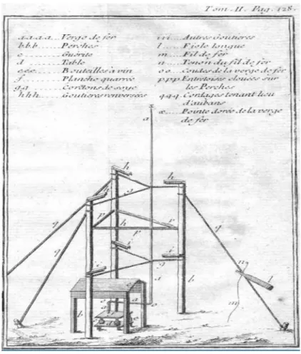
The apparatus used by Dalibard is presented in Figure 1.3; marked with (a) it is the metallic rod, as (g) the silk ropes, as (h) the protection against rain for the silk ropes and as (e) the wine bottles to ensure insulation from the ground. With this setup, it was possible to draw sparks from the rod or charge a Leyden jar.

Figure 1.3 Apparatus used by T.F.Dalibard for Benjamin’s experience. (Franklin, Expériences et Observations

(26)

After Dalibard successful experience, Benjamin Franklin in 1752 worked on the nature of the thunderclouds’ charge using what we know today as “Franklin bells”. Although, this instrument was an invention of Andrew Gordon, around 1740, a University teacher in Germany(Jefimenko, 1973).

Figure 1.4 Pierre-Charles Le Monnier portrait by Nicolas-Bernard Lépicié (http://fr.wikipedia.org).

Pierre-Charles Le Monnier, a French scientist, achieved the next breakthrough in this matter, reproducing Benjamin’s Franklin experience with few modifications, (Chambers, 1967). He used dust as an indicator of the experience objective and observed that the dust particles were attracted to the wire when it was electrified. However, the true discover he made was the fact that even in fair-weather, that phenomenon could happen; meaning that there also was a clear sky electrification. In 1753 John Canton, a member of Royal Society, did several experiments and built a new version of the electrometer at the time, which is documented by him in “Electrical Experiments, with an Attempt for account for their several Phenomena; together

with some Observations on Thunder-Clouds ”, and with this invention he studied the

electrification of thunderclouds. Also on that same year, he wrote a letter to the President of Royal society about his observations where he states two very interesting thing:

“The air without-doors I have sometimes known to be electrical in clear weather.”

Which is the same effect detected by Pierre-Charles Le Monnier, but he made a deeper study during different seasons of the year and accounted several different meteorological phenomena, leading him to say:

“[…] for in the succeeding months of January, February and March, my apparatus was electrified no less than twenty-five times, both positively and negatively, by snow, as well as by hail and rain.”

(27)

This statement shows that clouds were electrified both positively and negatively. At this point, the scientific community already knew that the clouds and the air itself are charged and that different meteorological phenomena can modify the charge state, in a positive or negative way. Later, several other scientist, worldwide,

kept working on this thematic, like Francesco Ludovico Beccaria, who begun in 1775 to measure daily variations in the atmospheric electricity, (Harrison, 2005), where he noticed the effect of fog and the positive electrification in fair-weather. He kept this task for several years and in 1789, John Read, driven by Beccaria’s work, made a two-year series of atmosphere electrification measurements (Harrison, 2005).

Figure 1.5 Giovanni Battista Beccaria portrait by Franz Joseph Anton von Thun-Hohenstein

(http://www.gettyimages.pt).

Working on the line of Beccaria was Horace Bénédict de Saussure (Switzerland), who found diurnal variations in atmospheric electricity, between 1785 and 1788, (Chauveau, 1925), reporting:

“In winter, the season during which I have the best observations of serene1 electricity…the electricity undergoes an ebb and flow like the tides, which increases and decreases twice in the span of twenty-four hours. The times of greatest intensity are a few hours after sunrise and sunset, and the weakest before sunrise and sunset”

Figure 1.6 Horace Bénédict de Saussure portrait by Jean Pierre Saint-Ours (http://www.summitpost.org).

With only primitive instruments, considering the ones existing today, it already could be seen a very distinct cycle in atmospheric electricity, which was going to be well defined only in 1920s through the Carnegie cruises. Nevertheless, it is very important to state that it was Charles Augustin Coulomb, who through experiments, noticed that a charge of an isolated

(28)

object decays to the air with time, (Leblanc, 2008). He did not have enough theoretical basis to explain this phenomenon, the electron was not yet been discovered, but he is credited as the one who discovered the electrical conductivity of the air, reporting:

“L’électricité des deux balles diminue un peu pendant le temps que dure l’experience… si l’air est humide et que l’électricité se perd rapidement [. . .]” (Coulomb, Mémoires sur l'électricité et le magnétisme, 1785).

After almost 80 years, in 1859 Lord Kelvin developed a new electric field sensor, usually called “water dropper potential equaliser” (Aplin and Harrison, 2013). On one hand, with this instrument he was able to measure what is known

today as potential gradient (PG1) related with the vertical component of the atmospheric electrical field. On the other hand, the method of photography recording was also discovered around that time and Lord Kelvin was able to build a system to obtain continuous measures of PG, known as Kelvin Electrograph. This system was used in several places like the Kew Observatory of London from 1861 to 1864 (Everett, 1868) and in the Eifel Tower (Harrison and Aplin, 2003).

Figure 1.7 Lord Kelvin portrait by Elizabeth King (http://www.docbrown.info).

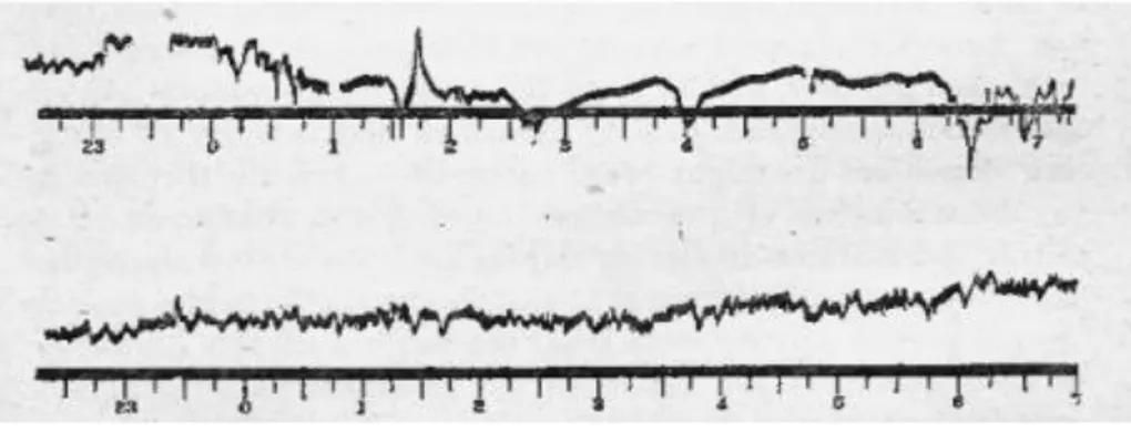
In Figure 1.8 is presented probably one of the first automatic and continuous records ever made of PG, measured in the Kew Observatory and that marked a new advanced in the study of atmospheric electricity and automatic measurements:

1_{The convention is that PG = dV}

I/dz, where VI is the potential difference between the Ionosphere and Earth’s

surface and z the vertical coordinate. It is defined to be positive for fair-weather and is related with the vertical component of the atmospheric electric field by Ez = PG.

(29)

Figure 1.8 Photographically recorded PG at Kew Observatory in 1861 (Aplin and Harrison, 2013).

After Lord Kelvin, there were crucial discoveries, which allowed the progress in atmospheric electricity science, like the one made by Wilhelm Conrad Roentgen who discovered the ionizing radiation in 1895 and the one by Joseph John Thompson in 1897 where he found what was called the electron.

Figure 1.9 a) J. J. Thompson portrait by George Fiddes Watt (http://www.bbc.co.uk); b) Wilhelm Conrad

Roentgen (http://www.nobelprize.org).

With various new instruments and through the development of science in all of its areas, Gerdien (1905a) was able to verify that air was slightly electrical conductive, just like Coulomb noticed. Gerdier also found that there was a current flowing from the upper atmosphere to the Earth’s surface and Charles Thompson Rees Wilson (Wilson 1906, 1908) built an apparatus to measure what was called as “air-Earth” current.

(30)

Figure 1.10 C.T.R Wilson portrait by James Gunn (http://www.sid.cam.ac.uk).

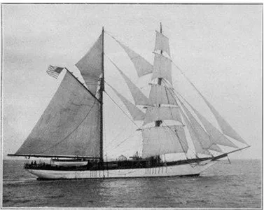
During 1920s, the Carnegie vessel sailed all over the world in order to make magnetic and electric measurements, specifically to measure PG. The ocean is an excellent location to make those measurements since it is less polluted than the continents and they found what is known as the Carnegie Curve, which is a characteristically PG variation curve. It was noticed that it was almost independent from the location where it was measured.

Figure 1.11 Carnegie vessel photograph courtesy of Carnegie Institution of Washington.

At this point, there was a lot of speculation about the source of this air current and the charging mechanism of earth’s surface and ionosphere and it was C.T.R. Wilson (1921, 1929) who proposed that the sources were thunderstorms and rain clouds (bad-weather regions).

(31)

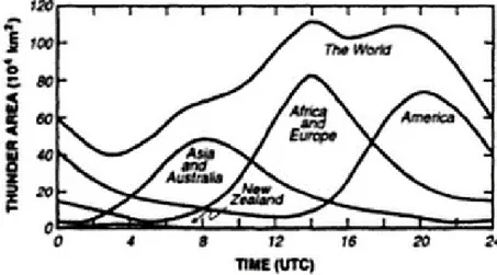
Since the beginning of the radio wave studies, it was known that the upper atmosphere was highly conductive so it was considered that the current was flowing from bad-weather to fair-weather regions, forming a global electric circuit, (Leblanc, 2008). Further proofs of this Global Electric Circuit (GEC) were found using measurements of the daily thunderstorm area, where it was found a strong positive correlation with the Carnegie Curve (Whipple and Scrase, 1936), see Figure 1.12 and Figure 1.13. At this stage, the basis of the present knowledge was built. Such knowledge is still growing today, with the study of new models for the Global Electric Circuit as well as the study of external factors impact on local PG.

Figure 1.12 Carnegie and Maud hourly averaged PG in % of mean (Whipple and Scrase, 1936).

Figure 1.13 Active Thunder area around the world (Whipple and Scrase, 1936).

Linss (1887) concluded that the negative charge of the Earth would leak away in a period of approximately 10 minutes when it was not maintained by any charge generating process in

(32)

the atmosphere. Israel and Kasemir (1949) calculated how fast a charge, which is injected into the atmosphere at a point P, distributes itself over a spherical shell with a given air conductivity around the globe. Israel (1957, 1970) made other calculations and concluded that the atmospheric electric equilibrium, at ground level, is reached in about 30 min. It is also known that the electric charge generated by a thunderstorm takes about 10 to 15 min to spread along the ionosphere around the all globe. This fact is the reason why hourly mean values are most common for investigation of the Global Electric Circuit.

1.2 Motivation

The study of the atmosphere, more concretely the study of its electrical properties as well as their effects, are a point of deep interest since it can be used to analyze natural phenomena related to humankind. Not only weather conditions can be retrieved from PG analysis but also the consequences of PG variations can dictate the start of, for example fires or fog events. The importance of PG is so vast in many different areas of society and it can be very handy in several situations that the curiosity to study it is too tempting.

In this context, Lisbon has vast records of PG measurements, from 1955 to 1991, which is a rare case. This situation provides the ideal opportunity to study a long time series and characterize Lisbon’s atmospheric electrical field. It is also of great importance since not much was done with this time series, which naturally improves its significance. Beside this, Lisbon also went through a long population and industrialization evolution, contributing to changes in the atmospheric electrical field among other things.Thus studding the PG records at Lisbon is a way of recovering its historical evolution, in particular in the 1980’s (after the democratic revolution).

On a deeper level, the study of things which humankind cannot see, at least at naked eye, but can measure, was from a certain point of my life not only a cause of motivation but also a continuous source of learning. The case of PG, among all other things that we cannot see at naked eye, made me think of what knowledge is and realize an important self-true about what

(33)

is called Engineering and Physics. One conclusion that I arrived was that knowledge cannot come only from books or whatever you may read.

Experience is and always will be a principal component for humans to understand nature, not only as a consequence to test theory results but also a cause to build theories. I also concluded another thing, which also came with my experience during my studies in the University of Évora, that there is only one object that, for humankind, provides the mechanism to understand the Universe where we live. That object is called mathematics and it rules almost everything we see and touch, excluding the things that even today we cannot even understand, and made me realize that there is no such thing as Engineering or Physics or anything else. These are divisions made by humankind to make easier for it to store the Knowledge in our own small minds. It does not matter if you called it Mechanics, Chemistry, Electricity or whatever.

In the end equations rules them all, even if slightly simplified. But the most important conclusion that I discovered is that all these subjects have one little thing in common with each other that most people cannot see or do not want to see, which is that they are all based in particles motion and interaction between them. If almost everything is motion and Mathematics, why not study the motion we cannot see but might be very important to society or actually have some usefulness or just because is just a thing that you want to learn more about? These are the questions, which led me to write this dissertation as an attempt to answer it.

1.3 Formulation of the global electric circuit

Thunderstorms, shower clouds and precipitation, cause separation of electric charge between the ground and ionosphere (also known as the equalizing layer), an electrically conductive layer about 60 km above the surface. This charge separation causes the ionosphere to have a potential (VI ) between 200 and 300 kV with respect to the Earth’s surface. Ionization from

(34)

near Earth’s surface), produces cluster ions (small ions) which make the atmosphere weakly electrical conductive. These ions flow vertically because of the vertical potential difference,

VI, causing the air-Earth conduction current density, JC, of order ~2 pAm-2. The total

electrical resistance for a unit area of the atmospheric column from the surface to the ionosphere is called the columnar resistance, RC and has value about ~ 300 PΩm2. A

schematic of the global circuit is given in Figure 1.14. Ohm’s law relates Ionosphere-Earth potential difference (VI), columnar resistance and air-Earth conduction current through the

equation:

The Ionosphere is positively charged with respect to the Earth’s surface under fair-weather conditions. This produces a downward pointing (negative) electric field (Ez), thus by

convention potential gradient (PG) is defined as the negative of Ez.

Near the Earth’s surface, the PG arises because JC is flowing through the weakly electrical

conductive air. It is therefore JC that permits the effect of the Global Electric Circuit (GEC)

circuit to be measured at the surface, either directly through the measurement of JC itself or

by PG.

However, PG is also a function of the local atmospheric air conductivity (σT). Away from

sources of charge separation, the atmospheric electrical conductivity (σT), potential gradient

and conduction current density are related by Ohm’s Law:

In the fair-weather part of the circuit, small ions dominate the charge transport since they have a large electrical mobility. Therefore, an increase in small ion concentration will increase the atmospheric electrical conductivity by providing more charge carriers. Aerosols in the atmosphere removes small ions by ion-aerosol coupling. An increase in aerosol number concentration therefore reduces the ion number concentration and decreases the atmospheric electrical conductivity. A change in aerosol number concentration subsequently modifies PG through Eq. (1.3).

𝑉𝐼 = 𝐽𝐶𝑅𝐶. Eq. (1.1)

𝑃𝐺 = −𝐸_𝑧. Eq. (1.2)

𝑃𝐺 = 𝐽𝐶

(35)

The global schematic of GEC and its important processes can be seen next on Figure 1.14:

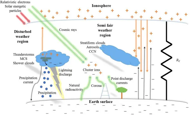
Figure 1.14 Processes of interest in the global electric circuit. Charge separation in thunderstorms, which

occur in disturbed weather regions, creates a substantial potential difference between the highly conducting regions of the ionosphere and the Earth’s surface. The positive potential of the ionosphere (positive with respect to the Earth’s surface) is distributed to fair-weather and semi-fair-weather regions, where a small current (whose density is JC) flows vertically. When this current flows through clouds it generates charge near the

upper and lower cloud edges, which can influence cloud microphysical processes. (In this diagram, Mesospheric Convective Systems, which are large scale thunderstorms late in their evolution and which favor sprite generation above them, are indicated by MCS; sprites are one example of Transient Luminous Events (TLEs); Cloud Condensation Nuclei are shown as CCN).

Thunder clouds, which generate potential differences exceeding 100 MV between the positive charges at their top sand the negative charges near their bottoms (Wormell, 1930), are one important source of upward currents through the atmosphere. They are both a DC ‘‘battery’’ and an AC generator in the circuit. Each one of the approximately 1000 thunderstorms active at any time generates an upward DC (Wilson) current of 1 A to the ionosphere, which is an excellent conductor, at an equipotential of 250 kV with respect to the Earth (e.g. Rycroft et al., 2000; Singh et al., 2011). The conduction current flows down in areas far from thunderstorms, termed regions of fair-weather (i.e. non-cloudy) and

(36)

semi-fair-weather (non-precipitating layer clouds). These currents flow through the partially conducting atmosphere where ionization is produced by galactic cosmic rays (GCRs); the vertical conduction current density is termed JC. Near the land surface, but not the oceans,

escaping radon determines the ion concentration and hence the electrical conductivity of the atmosphere in the planetary boundary layer, at heights up to 2 km (Pulinets, 2007; Kobylinski and Michnowski, 2007).

At sub-auroral latitudes, there is some extra ionization at 70 km altitude produced by relativistic (1 MeV) electron precipitation from the magnetosphere. Within the polar cap, polewards of the auroral oval, occasional energetic solar proton events (SPEs) of 100 MeV produce extra ionization at 60 km altitude. The circuit closes through the highly conducting land and sea, and via point discharge currents from pointed objects on the Earth’s surface up to the bottom of the thunderclouds. The increase by seven orders of magnitude of the electrical conductivity of the neutral atmosphere, from the Earth’s surface up to the lower ionosphere at 80 km altitude, has been modelled by Rycroft et al.(2007) and Rycroft and Odzimek (2010). It is emphasized here that the conductivity profile is the most important parameter in establishing the global circuit (Holzworth, 1987; Rycroft et al., 2008).

There is another important DC current generator in the global circuit; this is due to electrified rain/shower clouds (Figure 1.14) which generally bring negative charge to the Earth’s surface. The shower cloud contribution is believed to be a significant fraction (up to about a half) of that of thunderstorms.

Of the quantities, which can be measured at the surface, the air-Earth conduction current density (JC) presents one of the most fundamental parameters of the Global Electric Circuit

(Chalmers, 1967). In fair-weather regions, a positive current density occurs when positive charge moves downward and negative charges move upwards. The conduction current density is one of several components contributing to the total current density, JS, received by

a horizontal flat plate, conducting electrode, at the Earth’s surface, electrically isolated from the ground, like a PG measurement sensor. JS comprises contributions from turbulence JT,

(37)

conduction JC, displacement JD and precipitation JP. Based on Maxwell’s equations, the

displacement current density is given by:

where ϵ is the electric permittivity of air.

All precipitation particles carry positive or negative electric charges from the atmosphere to the ground. Precipitation current is very important from a global point of view, since it is one of the mechanisms for the maintenance of the negative electric charge on the Earth’s surface. Some measurements were made and amounts of ±0.2 up to 5×10-12 Am-2, (Reiter, 1976), were found. Bear in mind that this current depends strongly on the type, rate and physical state of the precipitation and weather conditions.

Finally fast electrons ionizing gas molecules induce point discharge current, which causes a strong local ion concentration increase. It can happen on the leaves of trees when a highly charged cloud is above them or it can happen by means of corona discharges.

1.4 Atmospheric Ions and interaction with aerosols

Aerosols can be defined as an assembly of liquid and/or solid particles suspended in the atmosphere and when they are substantially big, we can notice them as they scatter and absorb sunlight. The size distribution of these particles ranges from r > 3 nm, that corresponds to large ions (usually referred as charged aerosol particles) up to 100 μm, which is characteristic of large organic matter. Usually the aerosols can be divided into 2 groups accounting to their size: fine particles, d < 2.5 μm, and coarse particles, d > 2.5μm. Aerosols may be originated by several ways, being the most important ones affecting the Earth’s environment, volcanic aerosols, desert dust and anthropogenic aerosols, essentially from industry heating systems and traffic. These ones are referred as primary aerosols, because they are directly injected into the atmosphere. There are also secondary aerosols, which result from chemical interactions between several constituents of the atmosphere, which can be derived mainly by two methods: Gas-to-Particle Conversion, (GPC), which consists in gas 𝐽_𝐷 = 𝜖𝑑𝐸𝑧

(38)

molecules becoming clustered together, creating a macroscopic particle; Ion-Induced nucleation, which is a process based on aerosol formation and growth by vapor condensing onto an ion (CCN).

Atmospheric small ions both positive (n+) and negative (n-) are small clusters, which carry

electric charges through the air. Small ions have electric mobilities between 1 and 3 cm/s for 1 V/cm; large ions, between 3×10-3 and 3×10-4 cm/s for 1 V/cm; intermediate ions have electric mobilities between the values of the other two.

Small ions are the most important type of ions for atmospheric electricity; this is because they have high electric mobility, allowing them to take a more active part in charge transfer through the atmosphere. The electric mobility of ions is of great importance since it determines how much an ion contributes to the electric conductivity of the air. The positive and negative contribution of all particles to the atmospheric electric conductivity can be expressed in a general form by:

where z represents the height, μ represents the small ion electric mobility for both polarizations, n is the number density of positive and negative ions, K is the electric mobility of all larger ions (which goes from intermediate ions to charged aerosol particles), N corresponds to the number of large ions, p and m to the different diameters of particles and

υ, υ=1 for small ions, is the number of elementary charges e per ion size (larger particles can

bear more than 1 elementary charges, instead, small ions have always υ = 1).

Nevertheless, the equation for the total atmospheric electric conductivity is commonly simplified considering only small ions (as they have the greatest effect on it) and charged aerosol particles are assumed to have a negligible contribution (Wright et at., 2014a). Using this simplification and considering the total atmospheric electric conductivity, which means 𝜎₊(𝑧) = 𝑒𝜇₊(𝑧)𝑛₊(𝑧) + ∑ 𝐾₊𝑝(𝑧)𝑁(𝑧)₊𝑝𝜐₊𝑝𝑒, 𝑝 𝜎₋(𝑧) = 𝑒𝜇₋(𝑧)𝑛₋(𝑧) + ∑ 𝐾₋𝑚_(𝑧)𝑁 −𝑚(𝑧)𝜐−𝑚𝑒 𝑚 , Eq. (1.5)

(39)

the sum due to positive and negative ions and that both type of ions have the similar mobilities and number density we arrive at:

Woessner et al. (1958) made several measurements of ion conductivity of both polarization with respect to height, z, up to 26 km and found the following relations:

A plot of Eq. (1.7) is shown here:

Figure 1.15 Conductivity profile.

Primary ions, singly charged positive ions and free electrons, are mainly produced by ionization of molecules in the air and quickly form small ions clusters,through the clustering of water molecules, becauseit is energetically favorable for primary ions to react rapidly with water molecules. The sources attributed to play a role in atmospheric ionization are cosmic radiation and radon decay through gamma, alpha and beta radiation.

𝜎_𝑇(𝑧) = 𝜎+(𝑧) + 𝜎−(𝑧) ≅ 2𝜇(𝑧)𝑛(𝑧). Eq. (1.6)

𝜎+(𝑧) = 3.33 × 10−14exp(0.254𝑧 − 0.00309𝑧2), 𝜎−(𝑧) = 5.34 × 10−14exp(0.222𝑧 − 0.00255𝑧2).

(40)

The process of small ion cluster formations is explained as follows: upon a molecule or atom being hit by those ionization agents, it loses an electron per impact, leaving them positively charged and thereby forming a positive primary ion with one elementary charge. The free electron will be captured within ~10-8 seconds by a neutral molecule or atom forming a negative primary ion. The primary ions keep colliding with other molecules and atoms in the air for about 1010 times/s. The ones that are not removed by mutual recombination tend to form small ion clusters when water vapor is present (Reiter, 1976). The all process is represented schematically in Figure 1.16:

Figure 1.16 Schematic representation of small ion clusters formations.

Without exception, small ion clusters only carry one elementary charge and their life-time depends on aerosol particle concentration. Since both small ions and aerosol move in the air they can both collide with each other. The very important concept of “ion equilibrium” is composed by three basic components: 1) small ion production rate, q; 2) the recombination of the polar small ions, which then dissipate, expressed by the recombination coefficient α; 3) the attachment between small ions and air aerosols, expressed by the coefficient βa.

(41)

Equilibrium equations are shown next:

where n=n++n-, 𝑛̅= (n++n-)/2, N=N(Ra) corresponds to the concentration of all particles with

radius Ra. N0(Ra) corresponds to the concentration of uncharged particles with radius Ra.

Nυ=Nυ(Ra) corresponds to the concentration of positive and negative charged particles where

the index, υ, determines the amount of elementary charges. β0= β0(Ra) is the combination

coefficient between small ions and uncharged particles, βυe=βυe(Ra) is the combination

coefficient between small ions and charged particles with equal sign, e, with υ elementary charges and βυu=βυu(Ra) is the combination coefficient between small ions and charged

particles of unequal sign, u, with υ elementary charges.

Considering that all aerosol particles have an “effective radius”, i.e they form a representative monodisperse population, that no charged aerosol particles are present, the number of positive and negative ions is equal, expressed by n, 𝛽_𝑎is the effective ion-aerosol attachment coefficient, Za is the aerosol number concentration, Za is the aerosol number

concentration, Eq. (1.8) can be simplified to a single formula for ion balance:

From this equation, it is possible to calculate the evolution of the number of ions in an environment containing aerosols varying with time. The formalism developed by (Hoppel, 1985) uses effective parameters to simplify the equation for ion balance in the presence of a more realistic case that should consider the aerosol size distribution. This formalism gives theoretical support to the assumption made in Eq. (1.9) of a monodisperse aerosol 𝑑𝑛 𝑑𝑡 = 𝑞 − 𝛼𝑛̅2− 𝛽0𝑛̅𝑁0− 𝛽1𝑒𝑛̅𝑁1− 𝛽1𝑢𝑛̅𝑁1− 𝛽2𝑒𝑛̅𝑁2− 𝛽2𝑢𝑛̅𝑁2 𝑑𝑁0 𝑑𝑡 = 2𝛽1𝑢𝑛̅𝑁1− 2𝛽0𝑛̅𝑁0 𝑑𝑁1 𝑑𝑡 = 𝛽0𝑛̅𝑁0+ 𝛽2𝑢𝑛̅𝑁2− 𝛽1𝑢𝑛̅𝑁1− 𝛽1𝑒𝑛̅𝑁1 𝑑𝑁2 𝑑𝑡 = 𝛽1𝑒𝑛̅𝑁1+ 𝛽3𝑢𝑛̅𝑁3− 𝛽2𝑢𝑛̅𝑁1− 𝛽2𝑒𝑛̅𝑁1 𝑑𝑁3 𝑑𝑡 = 𝛽2𝑒𝑛̅𝑁2+ 𝛽4𝑢𝑛̅𝑁4− 𝛽3𝑢𝑛̅𝑁3− 𝛽3𝑒𝑛̅𝑁3, Eq. (1.8) 𝑑𝑛 𝑑𝑡 = 𝑞 − 𝛼𝑛2− 𝛽𝑎𝑍𝑎𝑛. Eq. (1.9)

(42)

distribution by using an “effective” ion-aerosol attachment coefficient βa as representative of

a polydisperse aerosol population. Thus, the steady-state equation for ion formation and loss in the presence of aerosols can be written as:

It is worth to mention here that Eq. (1.10) is a simplification because it neglects the positive to negative ion concentration unbalance which is crucial in highly perturbed regions where space charges form (Matthews et al., 2010). Nevertheless, the present formulation assumes a quasi-equilibrium state perturbed by the presence of aerosols. The solution of Eq. (1.10) is straightforward:

Further developments regarding this matter are discussed in the following chapters.

1.5 Dissertation structure

 Chapter 2 provides an insight of mathematical techniques and instruments used through the dissertation and a briefing about other formulations useful for Engineering, such as the Discrete Fourier Transformation and primitive instruments like Lord Kelvin’ Electrometer.

 Chapter 3 approaches a very important thematic, which is the effect of pollution on atmospheric electric field of Lisbon, where a daily and weekly cycle were identified on PG records. (This is a study, which is in vogue nowadays, since pollution is one of the major problems affecting society in several and problematic ways).

 Chapter 4 includes a deeper thematic, which is the relation between relative humidity, which can be an indicator of fogs, for instance, and the atmospheric electric field. A new model, according to some simplifications, is presented and shows a very close relation between PG and relative humidity when aerosols grow hygroscopically. (This information can maybe in the future be used for fog detection).

𝑞 − 𝛼𝑛2_{− 𝛽}

𝑎𝑍𝑎𝑛 = 0. Eq. (1.10)

(43)

 Chapter 5 corresponds to the study of one of the most severe tragedies that occurred in the recent history of Lisbon. This event was the Chiado’s fire and this study demonstrates the later effect of fire plume in the atmospheric electric field. This is the first study able to make a connection between the smoke plume dynamics and the

PG response to it, which is very important not only because it is the first, but also it

may enable, in the future, the study of smoke plume’s motion with PG records as an extra tool for fire fight or any other idea that may arise.

 Chapter 6 presents a simple circuit model of the Global Electric Circuit coupled with a local circuit, measuring PG in fair-weather conditions. This is a first attempt to connect both things in order to separate the global effects from the local ones and to find values that are suitable to compare literature values for the Global Electric Circuit parameters with real data. This chapter is a preliminary work and is referenced for future work and development.

(44)

2 Instrumentation

and

Signal

Processing

Techniques

2.1 Introduction

This chapter englobes the explanation of mathematical techniques and instruments used along the dissertation and a briefing about them.

2.2 Lord Kelvin’s Water Dropper apparatus

A fundamental atmospheric electrical measurement is to acquire the electric potential at a known height, from which the vertical potential gradient (PG) can be obtained. This requires that minimal distortion of the potential occurs from the measurement apparatus, or that a correction can be applied for the distortion, since objects disturb the electrical field.

Lord Kelvin developed two PG sensors but only one of his instruments will be briefed here. Kelvin water dropper equaliser instrument comprised an insulated tank of water from which a continuous stream of water is allowed to flow (for example, out of a window), finally breaking into water drops: The water tank and an electrometer to measure the tank’s potential would typically be installed on an upper floor of a building (Figure 2.1). At the stream to spray transition, droplets will polarize if their potential (which is that of the tank, via the connection provided by the water stream), differs from the local potential of the air. The effect of this polarization at the moment of drop release is to cause charge transfer between the water stream and the air, which continues until the potential of the water stream equals the potential of the air at the stream-spray transition point. Because the tank is connected through the water stream to the spray formation point, the formation point potential can be measured more conveniently at the tank. If the height of the stream-spray transition point is also determined, the vertical potential gradient can be found.

(45)

Figure 2.1 Schematic of water dropper equaliser (Gendle, 1912).

Lord Kelvin got even further and developed an automatic measurement system with the help of photographic paper and reflexion of light. A beam of light was reflected on a mirror, which was connected to the vane, which rotated based on the potential it acquired from air and the electrodes enclosing the vane. That beam of light was then reflected to photographic paper, where there was already a time and PG scale.

(46)

The zero was set as seen in Figure 2.2 and the basic scheme can be visualized on it.

Figure 2.2 Lord’s Kelvin Electrometer schematic (www.orau.org).

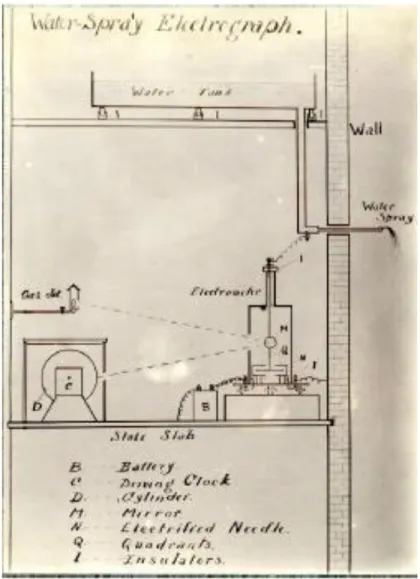
2.3 Benndorf Electrograph

A Benndorf electrograph was coupled to a radioactive probe to secure equality of potential between the sensor and the air and also improving the time response of the electrograph, since the radioactive decay impose an increase in ionization, allowing the sensor to measure small value fluctuations and at the same time a faster response . It was installed at 1 m above ground in a cement base recorded the PG at Portela meteorological station (Lisbon Airport, Portugal). Its sensitivity was checked using an electronic electrometer with standard voltage source between ± 200 V and the same calibration procedure was used in all periods of operation, from 1950’s to 1990’s. The analog records of the electrograph were digitalized afterwards (Serrano, 2010). Further details on the dataset can be found in (Serrano et al., 2006 and Serrano, 2011). Measurements with similar devices were made worldwide, e.g. (Shigeno et al., 2001).

This instrument was portable which is an advantage compared with the one from Lord Kelvin and data writing process was achieved through a telegraph technique.

(47)

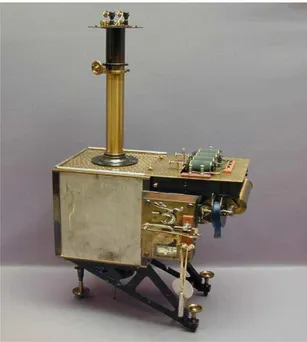
Figure 2.3 Benndorf’s Electrometer (http://physik.uibk.ac.at).

Sensor schematics can be seen next:

Figure 2.4 Benndorf’s Electrometer schematic (Klemens R., 2003).

The 20 cm long pointer Z of aluminum wire is rigidly connected with the needle of the quadrant electrometer. It swings across a 12 cm wide paper strip, which is moved about 4 cm

(48)

per hour through a clockwork. The pointer will be pressed down from time to time and marks its position. For this purpose it lies a knitting needle s below the paper strip, above the paper strip lies a strip of “blue paper”. If the stirrup H pressed the pointer down, a blue dot forms on the paper. Such so-called point recorder has the advantage of an almost non-existing hysteresis, therefore such recorders have been manufactured and distributed until the end of the 20thCentury.

The clockwork drives the roll W1 for the paper transport. The print roll W2 prohibits the slippage of paper; W3 is only a deflector roll. Batteries supplied the electromagnet. The core of the electrometer has been isolated from the pointer Z by a piece of amber b. The supply line to the needle was through the contact N and the platinum sheet p in sulphuric acid, which served for damping the system.

If the quadrant pair Q1, Q2 have been put to the potential V1, V2 and the moveable needle to the potential VN, there was a deflection of the pointer Z, where its intensity was determined by the torsional moment of the needle mounting was equally and opposing the moment evoked by the electrostatic forces. The measurements of the diagrams (paper roll) were carried out by glass scales.

2.2 Electric field mill JC 131/F

Because weather conditions are constantly changing, there exists a need to measure the strength of the electric field constantly, which translates into the need to alternately read the charged state of the sensor plate, discharge it, and read again, repeatedly. This is accomplished by repeatedly exposing the sensor plate to the external electric field to charge it, Figure 2.5(a), then shielding the plate to allow it to discharge, Figure 2.5(b). When the plate area is shielded, the charge on the plate must flow out, causing a current is to flow to

(49)

This current is proportional to the atmospheric field as:

where, As is the effective exposed area of the sensing electrode at the time t and ϵ is the

permittivity of air. If the induced signal is rectified by a phase-sensitive detector (relative to the shutter motion), the DC output signal will indicate both the polarity and magnitude of the electric field.

Figure 2.5 Field mill operating principle (http://www.missioninstruments.com).

One of the problems of this kind of sensor from Figure 2.5 is that the rotor connected to the chopper, needs to be connected to the ground to discharge, so the measurements are not disturbed by any potential created by on the unearthed rotor on the sensing plate. Late models used a system with brushed to ground the rotor, which is expensive at long terms and obviously the sensor needs to be stopped so the brushed can be replaced, leaving some data unrecorded. The JC1 131 uses a new system, called back to back, where the rotor does not need to be earthed. The ‘back to back’ fieldmeter approach, (Chubb, 1990) is based on two 𝑞_𝑠(𝑡) = 𝜖𝐸𝑧𝐴𝑠(𝑡), 𝑖𝑠(𝑡) = 𝜖𝐸𝑧 𝑑𝐴_𝑠 𝑑𝑡 , Eq. (2.1) a b