Contents lists available atScienceDirect
Journal
of
Mathematical
Analysis
and
Applications
www.elsevier.com/locate/jmaa
Computing
the
first
eigenpair
of
the
p-Laplacian
in
annuli
Grey Ercolea,∗,Júlio César do Espírito Santob, Eder Marinho Martinsb
a UniversidadeFederaldeMinasGerais,DepartamentodeMatemática,ICEx,Av.AntônioCarlos6627, CaixaPostal702,31270-901,BeloHorizonte,MG,Brazil
bUniversidadeFederaldeOuroPreto,DepartamentodeMatemática,ICEB,CampusUniversitário MorrodoCruzeiro,35400-000,OuroPreto,MG,Brazil
a r t i cl e i n f o a b s t r a c t
Articlehistory:
Received19March2014
Availableonline16September2014 SubmittedbyB.Kaltenbacher
Keywords:
Annulus Firsteigenpair
Inverseiterationmethod p-Laplacian
WeproposeamethodforcomputingthefirsteigenpairoftheDirichletp-Laplacian,
p>1,intheannulusΩa,b={x∈RN:a<|x|< b},N >1.Foreacht∈(a,b),we
use an inverse iteration method to solve two radial eigenvalue problems: one in the annulus Ωa,t, with thecorresponding eigenvalueλ−(t) and boundary conditions
u(a) = 0 = u′(
t); and the other in the annulus Ωt,b, with the corresponding
eigenvalue λ+(t) and boundary conditions u′(t) = 0 = u(b). Next, we adjust
theparameter tusinga matching procedureto make λ−(t) coincide withλ+(t),
thereby obtaining thefirst eigenvalueλp.Hence, by a simple splicingargument,
we obtain the positive, L∞-normalized, radial first eigenfunction u
p. The matching
parameteristhemaximumpointρofup.Inordertoapplythismethod,wederive
estimates for λ−(t) and λ+(t), andweprove that these functionsare monotone
and (locally Lipschitz) continuous. Moreover, we derive upper and lower estimates for themaximumpoint ρ,which weuseinthematchingprocedure, andwealso
presentadirectproofthatupconvergestotheL∞-normalizeddistancefunctionto
the boundary as p → ∞. We also present some numerical results obtained using thismethod.
© 2014ElsevierInc.All rights reserved.
1. Introduction
In this work, we consider the following eigenvalue problem
−∆pu=λ|u|p−2u, inΩa,b
u= 0 on∂Ωa,b,
(1)
* Correspondingauthor.
E-mailaddresses:[email protected](G. Ercole),[email protected](J.C. do Espírito Santo),[email protected]
(E.M. Martins).
http://dx.doi.org/10.1016/j.jmaa.2014.09.016
where ∆pu := div(|∇u|p−2∇u) is the p-Laplacian operator, p>1, and Ωa,b is the annulus
Ωa,b:=
x∈RN : 0< a <|x|< b, N >1.
It is well known that the first eigenvalue of the Dirichlet p-Laplacian in a bounded domain Ω ⊂ RN
is positive and it is also characterized as the minimum of the Rayleigh quotient ∇vpLp(Ω)
vp
Lp(Ω) taken over
all nontrivial functions v ∈ W01,p(Ω). Furthermore, the corresponding extremal functions, i.e., the first
eigenfunctions, do not change sign in Ω, are scalar multiples of each other (i.e., the first eigenvalue is
simple), and they belong to C1,τ(Ω) for some 0 < τ <1.
Wedenoteλpas thefirsteigenvalueof(1)andupasthepositiveandL∞-normalizedeigenfunctionthat
corresponds to λp. Thus,
λp= min
∇vp Lp(Ωa,b) vpL
p(Ωa,b)
: 0≡v∈W01,p(Ωa,b)
= ∇up
p Lp(Ωa,b) uppLp(Ωa,b)
,
up>0 inΩa,b andupL∞
(Ωa,b):= 1.
When the domain Ωis a ball or an annulus, the first eigenfunctions must be radially symmetric (see[21]). In particular, for the annulus Ωa,b, we have up=up(r), where r=|x|∈[a,b],
λp= min b
arN−1|v′(r)|pdr
b
arN−1|v(r)|pdr
: 0≡v∈W01,p(a, b)
= b
ar N−1|u′
p(r)|pdr
b
arN−1|up(r)|pdr
and up∈C1,τ([a,b]) ∩W01,p((a,b)) satisfies the boundary value problem
−rN−1u′p−2u′ ′ =λprN−1up−1, r∈(a, b)
u(a) = 0 =u(b). (2)
It is easy to check that up has a unique critical point ρ∈(a,b), where it attains its maximum value. Thus,
up(r) is strictly increasing if r∈[a,ρ), and strictly decreasing if r∈(ρ,b] and up(ρ) = 1 =upL∞([a,b]).
The properties of the first eigenpair of the Dirichlet p-Laplacian in an N-dimensional bounded domain Ω
arewell known,butthefirsteigenpair itselfisgenerallydifficultto compute,evenforsimpledomainssuch as a ball, a square, or an annulus, when 1 < p= 2 and N >1. In the last three decades, several studies have
aimed to improve the estimates of the first eigenvalue for general bounded domains, or proposed methods for the numerical computation of the first eigenpair for some domains (see [2–7,11,14,17,19]). In the present work, we propose a new method for computing the first eigenpair (λp,up) of the eigenvalue problem (1).
In[7], an iteration method was developed based on the inverse power method of linear algebra to compute the first eigenpair of the Dirichlet p-Laplacian in a ball. By exploiting the radial form of the first
eigenfunc-tion, this method produces sequences that converge rapidly and monotonically to the first eigenpair. In [6], another iterative method was proposed based on the sub-supersolution approach, which was shown to work for a general bounded domain and it was implemented for some simple cases. For nonradial domains, such as a square, a cube, or a torus, the implementation of this method used a regularization of the form div((ǫ2+|∇u|2)p−p2) for ∆
puin order to avoid the singularity or degeneracy at ∇u = 0.
The first step of both iterative processes uses the p-torsion function, where the solution of the following
problem is known as the “torsional creep problem” (see [16])
−∆pu= 1, inΩ
In the case where Ω is a ball, the p-torsion function is also radially symmetric and the corresponding
radial version of the torsional creep problem is rewritten as a boundary value problem for an ordinary differential equation (ODE) in the radial variable r. A simple examination of this ODE allows us to see that
the p-torsion function is strictly decreasing with respect to r. Hence, after two integrations (of the ODE),
we can easily obtain an explicit expression for the p-torsion function.
A similar procedure can be employed to solve the first eigenvalue problem in the unidimensional case (N = 1) for any p>1. In fact, in this case, Ω is an open interval (a,b) and both the p-torsion function
and the first eigenfunctions are symmetric with respect to their maximum point, which necessarily occur at the same place: the midpoint m := a+b2 . Therefore, as in the case of the ball, an explicit expression can be
derived for the p-torsion function, thereby making the inverse iteration method directly applicable (see [8]) to solving the eigenvalue problem in (a,m) or in (m,b), which allows us to obtain one of the halves of the
first eigenfunction. The other “half” is obtained by reflecting that found previously around m.
However, the p-torsion function is generally not expressed by a simple formula. Moreover, its numerical
computation is not simple if 1 < p= 2 and N >1. In some nonradial domains (see [6]), its computation demands significantly more interactions than the subsequent terms of the sequences that converge to the first eigenpair. It should be noted that the number of interactions that are necessary to produce good approximations of the p-torsion function seems to decrease with p, for large values of p, as mentioned in [6].
Even in the case of the annulus where N > 1 and 1 < p = 2, an explicit expression for the p-torsion
function is not available. Indeed, its radial form alone is not sufficient to produce such an expression after integrating the corresponding ODE boundary value problem. This is because the position of its maximum point is not known a priori. Moreover, the maximum points in the subsequent iterations change during each step, thereby making the computations longer and more difficult. Consequently, inverse iteration starting from the p-torsion function does not appear to be suitable for computing the first eigenpair of the annulus Ωa,b if we want to explore its radial symmetry.
We computethefirsteigenpairofΩa,bbyexploitingitsradialsymmetrytosplitthecorrespondingradial
eigenvalue problem into two simpler ones. However, this strategy makes the maximum point ρan additional
unknown (beyond λp and up) in our problem.
In particular, our method for computing the first eigenpair of (1) involves splitting the first eigenvalue problem for Ωa,b into two radial problems that are determined by the splitting parameter t∈(a,b), which
should converge to ρ. The “left” radial eigenvalue problem is posed in Ωa,twhere the first eigenpair is denoted
by (λ−(t),u−(t,·)) and the“right” radialeigenvalue problem is posed in Ωt,b where thefirst eigenpair is
denoted by (λ+(t),u+(t,·)).
Each of these radial eigenvalue problems has the same structure as the radial eigenvalue problem for a ball. Next, we apply the inverse iteration method to compute the first eigenpairs (λ−(t),u−(t,·)) and
(λ+(t),u+(t,·)) and we use a matching procedure to adjust the parameter t to the maximum point ρ, i.e.,
to that which makes λ−(t) =λ+(t) =λp. This allows us to splice u−(t,·) with u+(t,·), thereby forming
the first eigenpair up of the annulus. The numerical implementation of this script does not require any
regularization of the p-Laplacian.
In order to provide theoretical support for the procedure described above, we explore the variational characterization of the first eigenvalues to prove the continuity of the functions λ−(t) and λ+(t), their
behavior at the endpoints a and b, and the following explicit bounds for the unknown maximum point ρ,
which is a relevant issue for starting the matching procedure:
b+a[(b
a)N−1+ ( b a)N+ 1]
1 p
1 + [(b
a)N−1+ ( b a)N+ 1]
1 p
< ρ < a+b
2 . (3)
As a byproduct, these bounds show that ρtends to the midpoint m = a+b2 as p→ ∞, which then allows us
lim
p→∞up=
δ δ∞
, uniformly inΩa,b, (4)
where
δ(x) :=
|x| −a; ifa≤ |x| ≤m b− |x|; ifm≤ |x| ≤b
is the distance function of xto the boundary of Ωa,b.
The convergence (4) can also be verified by combining some results on the Dirichlet eigenvalue problem for the ∞-Laplacian operator in a bounded domain Ω ⊂ RN. In fact, it was proved in [15] that at least one subsequence of the family { up
upL1 (Ω)}p>1 exists that converges uniformly in Ω to a function u∞ and
that any such a limit function is a positive viscosity first eigenfunction of the Dirichlet ∞-Laplacian. In
addition, for some special domains, such as balls, annuli, and stadiums, it was shown in [23]that the distance function to the boundary is the only viscosity first eigenfunction of the Dirichlet ∞-Laplacian in Ω, up to
some constant factor.
To the best of our knowledge, there have been no previous reports of explicit computations of the first eigenvalue for multidimensional annuli when 1 < p = 2. The only previous work to deal with the computation of the radial eigenvalues in multidimensional annuli is [9], where the authors considered a more general radial p-Laplacian eigenvalue problem in the framework of the Sturm–Liouville problem. They
developed a numerical method to compute the radial eigenpairs by transforming the second-order ODE into a first-order system (using a generalized Prüfer transformation), where they applied shooting algorithms and Newton’s method. Their method also depends greatly on the calculus of the generalized sine function introduced in [13] (see also [20]). The advantage of our method is that it is straightforward when applied to the Dirichlet eigenvalue problem for a genuine annulus (0 < a< b), where our approach only depends
on the integral formulae obtained by direct integration of the radial boundary value problems posed in Ωa,t
and Ωt,b. Unfortunately, we could not compare our outputs with those reported in [9]because the Dirichlet
eigenvalue problem for a genuine annulus was not among the numerical results that the authors used to illustrate their method. However, it is interesting to note that the numerical results presented in [7,Table 1] for the first eigenvalue of the unit ball are highly comparable with the corresponding results presented in [9,Table 4], where they agree up to the third decimal digit.
We should also note that our method can be treated as a routine for computing the first eigenpairs for a finite number of annuli that correspond to a partition of the interval [a,b], and thus it can be used to compute
any radial eigenpair of the annulus Ωa,b. For example, in order to compute the second radial eigenpair, we
can apply our method to each t ∈ (a,b) to calculate the Dirichlet first eigenpairs (γ−(t),u−(t,·)) and (γ+(t),u+(t,·)) of the annuli Ωa,tand Ωt,b, respectively. Hence, we adjust csuch that γ−(c) =γ+(c) and we
take this value as the second radial Dirichlet eigenvalue of Ωa,b(we know from [12]that the jth-eigenfunction
has exactly j−1 zeroes in (a,b)). The second radial eigenfunction is then obtained by splicing u−(c,·) with
ku+(c,·), where k:= u ′
−(c,c) u′
+(c,c) guarantees a C
1 contact at the root r=c. The constant k can be computed
easily from the integral expressions of the derivatives u′
±(c,c). This script can also be used to compute any radial eigenpair of a ball by combining our method with that employed in [7]. At this point, we should emphasize that an eigenfunction associated with the second eigenvalue of a radially symmetric domain can be nonradial. In fact, the second eigenfunctions of the p-Laplacian in a planar disc are not radial, according
to [22]for p = 2 and [5]for all p>1.
The remainder of this paper is organized as follows. In Section2, we specify the notations used in this study. In Section 3, we combine scaling arguments with variational characterizations of λp to derive the a priori bounds (3)for the maximum point ρof up. In this section, we also use similar arguments to prove
that the functions λ−(·) and λ+(·) are strictly monotone and (locally Lipschitz) continuous, as well as to
method developed in [7]to compute the eigenpairs (λ−(t),u−(t,·)) and (λ+(t),u+(t,·)) for each t∈(a,b).
In Section 5, we use a L’Hôspital rule for monotonicity (see Lemma 13) to obtain the lower and upper bounds for the first eigenfunction upin terms of explicit functions that depend on p, and hence we prove the
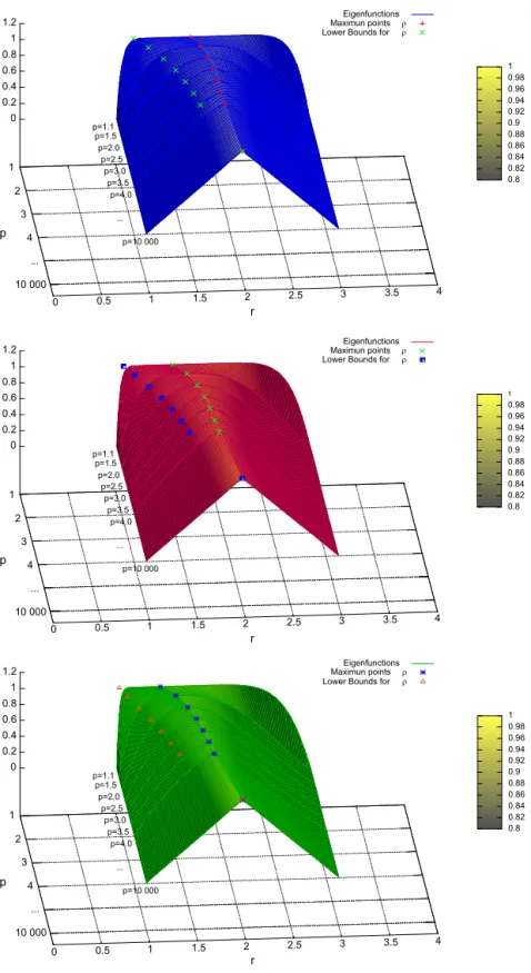
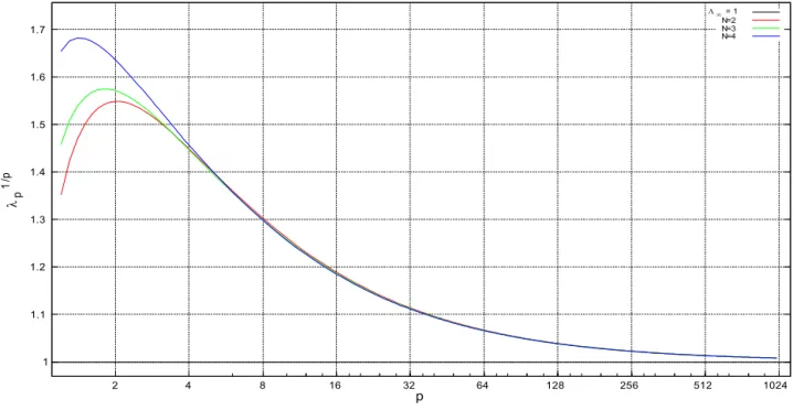
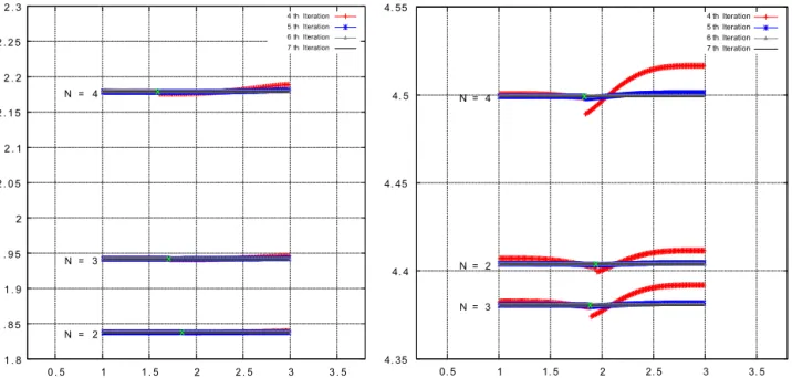
convergence (4). Finally, in Section6, for several values of pand N, we present numerical approximations
of λp and the corresponding graphs of up. These numerical results endorse the well-known asymptotic
behaviors of the first eigenpair (when pgoes to 1 and when pgoes to ∞).
2. Preliminariesandnotations
We recall that ρdenotes the maximum point of the first eigenfunction up. It is simple to check that λp
is also the first eigenvalue of both eigenvalue problems
−rN−1w′p−2w′ ′ =λrN−1wp−1, a < r < ρ
w(a) = 0 =w′(ρ) (5)
and
−rN−1w′p−2w′ ′ =λrN−1wp−1, ρ < r < b
w′(ρ) = 0 =w(b). (6)
In addition, the restriction of up to the interval [a,ρ] is an eigenfunction of (5)corresponding to λp as well
as up restricted to [ρ,b] is an eigenfunction of (5)corresponding to λp.
In fact, both of these eigenvalues problems have the following property: the only eigenfunction that does not change its sign is the first.
Therefore,λp canalsobe writtenas
λp= min ρ ar
N−1|w′(r)|pdr
ρ
arN−1|w(r)|pdr
: 0≡w∈C1[a, ρ] such thatw(a) = 0 =w′(ρ)
(7)
as well as
λp= min b
ρsN−1|w′(s)|pds
b
ρsN−1|w(s)|pds
: 0≡w∈C1[ρ, b] such thatw′(ρ) = 0 =w(b)
. (8)
After integrating (5)with λ =λp and w=up, we also obtain
0< u′p(r) =
λpr1−N ρ
r
σN−1u
p(σ)p−1dσ
1
p−1
, a≤r < ρ (9)
and
up(r) = r
a
λpθ1−N ρ
θ
σN−1up(σ)p−1dσ
1
p−1
dθ, a≤r≤ρ. (10)
Analogously, after integrating (6)with λ =λpand w=up, we obtain
0<−u′p(r) =
λpr1−N r
ρ
σN−1up(σ)p−1dσ
1
p−1
and
up(r) = b
r
λpθ1−N θ
ρ
σN−1up(σ)p−1dσ
1
p−1
dθ, ρ≤r≤b. (12)
In order to clarify our method for computing the first eigenpair (λp,up), we need to provide some
definitions.
For each a< t< b, we denote λ−(t) as the first eigenvalue associated with the eigenvalue problem
−rN−1w′p−2w′ ′=λrN−1wp−1, a < r < t
w(a) = 0 =w′(t) (13)
and u−(t,r) is the corresponding positive first eigenfunction such that
u−(t,·)
∞:= maxa≤r≤tu−(t, r) = 1.
Analogously,we denoteλ+(t) asthefirsteigenvalueassociatedwiththeeigenvalueproblem
−rN−1w′p−2w′ ′=λrN−1wp−1, t < r < b
w′(t) = 0 =w(b) (14)
and u+(t,r) is the corresponding positive first eigenfunction such that
u+(t,·)
∞:= maxt≤r≤bu+(t, r) = 1.
The eigenfunctions u−(t,·) and u+(t,·) belong to the class C2 in the closed intervals [a,t] and [t,b] if
1 < p ≤ 2 and they belong to C1,p−11 in these intervals if p> 2. It is also easy to check that u−(t,·) is
strictly increasing whereas u+(t,·) is strictly decreasing.
The eigenvalues λ−(t) and λ+(t) are positive and they satisfy, respectively,
λ−(t) = min 0≡w∈C1([a,t]) w(a)=0=w′
(t)
t ar
N−1|w′(r)|pdr
t
arN−1|w(r)|pdr
= t
ar N−1|u′
−(t, r)|pdr
t
arN−1|u−(t, r)|pdr
(15)
and
λ+(t) = min
0≡w∈C1([t,b])
w′
(t)=0=w(b)
b t r
N−1|w′(r)|pdr
b
t rN−1|w(r)|pdr
= b
t r N−1|u′
+(t, r)|pdr
b
t rN−1|u+(t, r)|pdr
. (16)
Of course,
λ−(ρ) =λp=λ+(ρ) and up(r) =
u−(ρ, r) ifa≤r≤ρ
u+(ρ, r) ifρ≤r≤b.
(17)
Remark1. As shown in Section3, the function Λ(t) :=λ−(t) −λ+(t) is (locally Lipschitz) continuous and
strictly decreasing in the interval (a,b), and it satisfies
lim
t→a+Λ(t) = +∞ and t→limb−Λ(t) =−∞.
3. Estimates andproperties oftheeigenpairs(λ±(t),u±(t,·))
In this section we derive lower and upper bounds for ρ and we study the behavior of the pairs
(λ±(t),u±(t,·)) with respect to t∈(a,b).
Lemma2.Suppose 0 ≤R1< R2 andthatu∈C2((R1,R2))satisfies
−τN−1u′(τ)p−2u′(τ) ′=τN−1fu(τ) ; R1< τ < R2,
wherethefunctionf iscontinuous.Consider thefollowingfunction
v(r) :=us(r) ; R1< r < R2,
where
s(r) =αr+β, R1< r < R2
fortheconstantsαandβ suchthat min{αR1+β,αR2+β}≥0. Then,
−rN−1v′(r)p−2v′(r) ′ =−(N−1)βr
N−2
s(r)
v′(r)p−2v′(r) +|α|prN−1fv(r) ; R1< r < R2.
Proof. We have
−rN−1v′(r)p−2v′(r) ′ =−|α|p−2αrN−1u′s(r) p−2
u′s(r) ′
=−|α|p−2α
r s(r)
N−1
s(r)N−1u′s(r) p−2
u′s(r) ′
=−|α|p−2α
r s(r)
N−1′
s(r)N−1u′s(r) p−2u′s(r)
− |α|p−2α
r s(r)
N−1
αd ds
sN−1u′(s)p−2u′(s)
s=s(r)
=−|α|
p−2α(N−1)βrN−2
s(r)
u′s(r) p−2u′s(r)
+|α|p−2α2
r s(r)
N−1
s(r)N−1fus(r)
=−(N−1)βr
N−2
s(r)
v′(r)p−2v′(r) +|α|prN−1fv(r) ,
where we have used
r s(r)
N−1′
s(r)N−1= (N−1)
r s(r)
N−2
s(r)−αr s(r)2 s(r)
N−1=(N−1)βrN−2
s(r) . ✷
Proposition 3.The followingupperboundforρholds:
ρ <a+b
2 . (18)
Proof. We use Lemma 2 with R1 = a, R2 = ρ, u = up, f(ξ) = λpξp−1, and the constants α and β are
defined by
α= ρ−b
ρ−a <0 and β =ρ
b−a ρ−a >0.
Note that the graph of the function
s(r) =αr+β∈[ρ, b], a≤r≤ρ
is the straight line connecting the points (a,b) and (ρ,ρ) on the rs-plane. Thus, the function
v(r) :=ups(r) , a≤r≤ρ
satisfies v(a) = 0, v′(ρ) = 0, v′(r) =u′p(s(r))α >0 whenever a≤r < ρ. Moreover, v∈C1([a,ρ]) ∩C2([a,ρ)).
Therefore, byLemma 2, wehave
−rN−1v′(r)p−2v′(r) ′=−(N−1)βr
N−2
s(r)
v′(r)p−1+|α|prN−1λ
pv(r)p−1, a < r < t. (19)
Hence, after multiplying this equality by v and integrating, we obtain
ρ
a
rN−1v′(r)pdr=−(N−1)β
ρ
a
rN−2
s(r)
v′(r)p−1v(r)dr+λp|α|p ρ
a
rN−1v(r)pdr
< λp|α|p ρ
a
rN−1v(r)pdr.
Now, by considering (15)and (17), we obtain
λp ≤
ρ a r
N−1|v′(r)|pdr
ρ
a rN−1v(r)pdr
< λp|α|p=λp
b−ρ ρ−a
p
and hence we arrive at
1< b−ρ
ρ−a. (20)
This leads directly to (18). ✷
Remark4. In the unidimensional case (N= 1), we can see from (19)that vis a positive eigenfunction that
corresponds to the eigenvalue λp|α|p. This fact implies that |α| = 1 and ρ = a+b2 .
Proposition5.The followinglowerbound forρholds:
b+a[(b
a)N−1+ ( b a)N+ 1]
1 p
1 + [(b
a)N−1+ ( b a)N+ 1]
1 p
< ρ. (21)
Proof. Following from the idea of the previous proof, we define
v(r) :=up
s(r) , ρ≤r≤b,
where
s(r) =αr+β ∈[a, ρ], ρ≤r≤b,
α=−ρ−a
b−ρ <0 and β=ρ b−a b−ρ =ρ
1 +|α| >0.
The graph of s is the straight line connecting points (b,a) and (ρ,ρ) on the rs-plane. Thus, v(b) = 0, v′(ρ) = 0 and v′(r) =u′(s(r))α <0 whenever ρ< r≤b.
Then, it follows from Lemma 2that
−rN−1v′(r)p−2v′(r) ′= (N−1)βr
N−2
s(r)
v′(r)p−1+|α|prN−1λ
pv(r)p−1, ρ < r < b. (22)
Hence, after multiplying this equality by v and integrating, we obtain
b
ρ
rN−1v′(r)pdr= (N−1)β
b
ρ
rN−2
s(r)
v′(r)p−1v(r)dr+λp|α|p b
ρ
rN−1v(r)pdr.
Now, according to (8), we obtain
λp≤
b ρr
N−1|v′(r)|pdr
b
ρ rN−1v(r)pdr
= (N−1)β b
ρ rN−2
s(r) |v′(r)|p−1v(r)dr
b
ρrN−1v(r)pdr
+λp|α|p. (23)
In addition, by combining (9)with the monotonicity of up(s) for s∈[a,ρ], we obtain
v′(r)p−1v(r) =|α|p−1u′ p
s(r) p−1up
s(r)
=|α|p−1up
s(r)
λps(r)1−N ρ
s(r)
σN−1up(σ)p−1dσ
=|α|p−1
λp ρ
s(r)
σ s(r)
N−1
ups(r) up(σ)p−1dσ
≤λp|α|p−1 ρ
s(r)
ρ a
N−1
up(σ)pdσ
=λp|α|p−1
ρ a
N−1 ρ
s(r)
After changing the variables σ=s(τ) in the latter integral, we obtain
v′(r)p−1v(r)≤λp|α|p−1
ρ a
N−1ρ
r
v(τ)pαdτ
=λp|α|p
ρ a
N−1r
ρ
v(τ)pdτ
≤λp|α|p
ρ a
N−1b
ρ
v(τ)pdτ
≤λp|α|p
ρ a
N−1b
ρ
τ ρ
N−1
v(τ)pdτ
=λp|α|pa1−N b
ρ
τN−1v(τ)pdτ
and hence we obtain
(N−1)βρb rs(r)N−2|v′(r)|p−1v(r)dr
b
ρrN−1v(r)pdr
≤(N−1)βλp|α|pa1−N b
ρ
rN−2 s(r)dr
≤βλp|α|pa1−N(N−1) b
ρ
rN−2
a dr
=ρ1 +|α| λp|α|pa−N
bN−1−ρN−1
< λp|α|p
1 +|α| b
N−1
aN
a+b
2
,
where we used ρ< a+b2 in the latter inequality.
By substituting this estimate into (23), we arrive at
kp≤
1 +1
k
bN−1 aN
a+b
2
+ 1,
where k:=|α|−1= b−ρ ρ−a.
According to (20), k >1. Hence,
b−ρ ρ−a
p
=kp
≤
1 + 1
k
bN−1
aN
a+b
2
+ 1
<2b
N−1
aN
a+b
2
+ 1 =
b a
N−1
+
b a
N
+ 1.
b−ρ ρ−a <
b a
N−1
+
b a
N
+ 1 1
p ,
from which (21)follows. ✷
It is interesting to note that our estimates (21)and (18)yield the following bounds for the quotient ρa in termsofthequotient b
a:
(ba) + [(ab)N−1+ (b
a)N+ 1]
1 p
1 + [(b
a)N−1+ ( b
a)N+ 1]
1 p
≤ ρ a ≤
1 + (ba)
2 .
Remark6. It follows immediately from estimates (18)and (21)that
lim
p→∞ρ=
a+b
2 . (24)
As mentioned in the Introduction, this asymptotic behavior is to be expected from the convergence (4), which can be obtained by combining a result on the existence in [15]with a result on the uniqueness in [23]. We use (24)in Section5to obtain a direct proof of (4).
In the sequel, we prove some properties for the functions λ−and λ+defined in (15)and (16), respectively.
First, we prove a monotonicity result, which implies that the function Λ(t) = λ−(t) −λ+(t) is strictly
decreasing in the interval (a,b).
Lemma7.Thefunctionλ−isstrictlydecreasingintheinterval (a,b]andthefunctionλ+isstrictlyincreasing intheinterval [a,b).
Proof. Suppose a< t1< t2≤b and define
u(r) =
u−(t1, r) ifa≤r≤t1
1 ift1≤r≤t2.
Obviously, u∈C1([a,t2]), u(a) = 0 =u′(t2). Thus,
λ−(t2)≤
t2
a r
N−1|u′(r)|pdr
t2
a rN−1|u(r)|pdr
=
t1
a r N−1|u′
−(t1, r)|pdr
t1
a rN−1|u−(t1, r)|pdr+
t2 t1 r
N−1dr <
t1
a r N−1|u′
−(t1, r)|pdr
t1
a rN−1|u−(t1, r)|pdr
=λ−(t1),
thereby showing that λ− is strictly decreasing in the open interval (a,b]. The proof of the monotonicity of λ+ is analogous. ✷
In the remainder of this section, we use the following formulae, which can be derived easily by integrating (13)and (14):
u′−(t, r)p−1=λ−(t)r1−N t
r
σN−1u−(t, σ) p−1
u−(t, r) = r
a
λ−(t)θ1−N t
θ
σN−1u−(t, σ) p−1dσ
1
p−1
dθ, a≤r≤t (26)
u′+(t, r)p−1=λ+(t)r1−N r
t
σN−1u+(t, σ) p−1
dσ, t≤r≤b
and
u+(t, r) = b
r
λ+(t)θ1−N θ
t
σN−1u+(t, σ) p−1
dσ
1
p−1
dθ, t≤r≤b. (27)
The next result shows the behavior of the function Λ(t) =λ−(t) −λ+(t) when t tends to the endpoints
of the interval (a,b).
Lemma 8.The followinglowerestimateshold
N aN−1
(tN−aN)(t−a)p−1 ≤λ−(t), a < t≤b (28)
and
N tN−1
(bN−tN)(b−t)p−1 ≤λ+(t), a≤t < b. (29)
Proof. Since u−(t,·)∞=u−(t,t) = 1, it follows from (26)that
1 =
t
a
λ−(t)θ1−N t
θ
σN−1u−(t, σ) p−1
dσ
1
p−1 dθ
≤
t
a
λ−(t)a1−N t
a
σN−1dσ
1
p−1
dθ=
λ−(t)
N
tN−aN aN−1
1
p−1
(t−a),
from which (28)follows.
Analogously, we obtain (29)by using (27). ✷
Proposition 9.Leta< x≤y < b.Then,
0≤λ−(x)−λ−(y) λ−(x)
≤ λ−(x)−λ−(y) λ−(y)
≤ C(y−x)
(x−a)p+N−1 +
1 + y−x
x−a
p
−1, (30)
where
C:= (N−1)b
N−2
aN−1(b−a)
p+N−1. (31)
Proof. The first and second inequalities derive from the monotonicity of λ−(t). In order to prove the third inequality, let us define the function
where s(r) =αr+β ∈[a,y], with
α= y−a
x−a >0 and β=a
x−y x−a <0.
We note that
s(a) =a and s(x) =y,
that is, the graph of s(r) is the straight line connecting the points (a,a) and (x,y) on the rs-plane. We have v(a) = 0,v′(x) = 0 and
v′(r) =u′−y, s(r) α >0, a≤r < x.
From Lemma 2, we also have
−rN−1v′(r)p−1 ′=−(N−1)βr
N−2
s(r) v
′(r)p−1+αprN−1λ
−(y)v(r)p−1.
By multiplying this equation by v(r) and integrating we obtain
x
a
rN−1v′(r)pdr=−(N−1)β
x
a
rN−2
s(r)v
′(r)p−1v(r)dr+αpλ −(y)
x
a
rN−1v(r)pdr.
It follows that
λ−(y)≤λ−(x)≤
x a r
N−1v′(r)pdr
x
a rN−1v(r)pdr
=(N−1)|β| x
a rN−2
s(r)v′(r)p−1v(r)dr
x
a rN−1v(r)pdr
+αpλ−(y), (32)
where the first inequality is due to the monotonicity of the function λ−(·) and the second inequality derives from the minimizing property of λ−(x).
Weremarkfrom (25),with t=y,that
u′−y, s(r) p−1=λ−(y)s(r)1−N y
s(r)
σN−1u −(y, σ)
p−1
dσ.
Hence,
v′(r)p−1v(r) =αp−1u′ −
y, s(r) p−1u−y, s(r)
≤αp−1λ−(y)
a1−N
y
s(r)
σN−1u−y, s(r) u−(y, σ)p−1dσ
≤ α
p−1λ −(y)
aN−1 y
a
σN−1u−(y, σ)pdσ,
Now, after changing σ=s(τ) in the latter integral and noting that β <0, we obtain
v′(r)p−1v(r)≤αp−1λ−(y)
aN−1 y
a
σN−1u−(y, σ)pdσ
=α
pλ −(y)
aN−1 x
a
s(τ)N−1v(τ)pdτ
=α
pλ −(y)
aN−1 x
a
(ατ+β)N−1v(τ)pdτ
≤α
p+N−1λ −(y)
aN−1 x
a
τN−1v(τ)pdτ.
Therefore,
(N−1)|β|
x
a
rN−2
s(r)v
′(r)p−1v(r)dr≤ (N−1)|β|xN−2
a
x
a
v′(r)p−1v(r)dr
≤ (N−1)|β|x
N−2
a (x−a)
αp+N−1λ−(y)
aN−1 x
a
τN−1v(τ)pdτ,
thereby implying that
(N−1)|β|axrN−2
s(r) v′(r)p−1v(r)dr
x
a rN−1v(r)pdr
≤ (N−1)|β|x
N−2
a (x−a)
αp+N−1λ−(y)
aN−1
≤ (N−1)|β|b
N−2
aN (x−a)α
p+N−1λ −(y)
= (N−1)a|x−y| x−a
bN−2 aN (x−a)
y−a x−a
p+N−1
λ−(y)
≤(N−1)b
N−2
aN−1(b−a)
p+N−1λ−(y)(y−x) (x−a)p+N−1
= Cλ−(y)(y−x) (x−a)p+N−1 ,
where C is given by (31).
Finally, we combine this estimate with (32)to obtain
λ−(y)≤λ−(x)≤
x a r
N−1v′(r)pdr
x
a rN−1v(r)pdr
≤
C(y−x) (x−a)p+N−1 +
y−a x−a
p
λ−(y)
and hence (30)follows. ✷
Proposition 10.Leta< x≤y < b.Then,
0≤ λ+(y)−λ+(x) λ+(y) ≤
λ+(y)−λ+(x)
λ+(x) ≤
1 + y−x
b−y
p
Proof. The monotonicity of the function λ+(·) yields both the first and second inequalities. The third
inequality follows in a similar manner as in the previous proof, although it is slightly simpler. In fact, we define the function
v(r) =u+x, s(r) , y≤r≤b
with s(r) =αr+β ∈[x,b] and
α= b−x
b−y >0 and β=b x−y b−y <0.
Here, the graph of s(r) is the straight line connecting the points (y,x) and (b,b) on the rs-plane. By applying Lemma 2, we obtain
−rN−1v′(r)p−2v′(r) ′=−(N−1)|β|r
N−2
s(r)
v′(r)p−1+αprN−1λ+(x)v(r)p−1.
(Note that v′ ≤0.) After multiplying the latter equation by v(r) and integrating, we obtain
b
y
rN−1v′(r)pdr=−(N−1)|β|
b
y
rN−2
s(r)
v′(r)p−1v(r)dr+αpλ+(x) b
y
rN−1v(r)pdr
≤αpλ+(x) b
y
rN−1v(r)pdr.
Therefore,
λ+(x)≤λ+(y)≤
b y r
N−1v′(r)pdr
b
yrN−1v(r)pdr
≤αpλ+(x) =
b−x b−y
p
λ+(x)
and(33)follows. ✷
The following corollary is an immediate consequence of Propositions 9 and 10.
Corollary11. Thefunctions λ−,λ+: (a,b) →(0,∞) are(locallyLipschitz) continuous.
Theorem12. Thefollowingclaims holdtrue:
1. λ−(ρ) =λ+(ρ) =λp.
2. λ−(t) > λ+(t)ifa< t< ρ.
3. λ−(t) < λ+(t)ifρ< t< b.
4. up(r) =
u−(ρ,r) if a≤r≤ρ u+(ρ,r) if ρ≤r≤b.
Proof. The function Λ(t) =λ−(t) −λ+(t) is continuous at any t∈(a,b) according to Corollary 11. Moreover, it follows from Lemma 7that this function is strictly decreasing and from Lemma 8that
lim
Therefore, a unique value of texists such that λ−(t) =λ+(t). Since we already know that λ−(ρ) =λ+(ρ),
we can conclude that such a value must be ρ, thereby proving the first claim. The second and third claims
follow directly from the first given the monotonicity of Λ(t). Since the positive function
v(r) =
u−(ρ, r) ifa≤r≤ρ
u+(ρ, r) ifρ≤r≤b
belongs to C1([a,b]), and it satisfies max
a≤r≤bv(r) = 1 and
b ar
N−1|v′(r)|pdr
b
arN−1|v(r)|pdr
= ρ
ar N−1|u′
−(ρ, r)|pdr+
b ρr
N−1|u′
+(ρ, r)|pdr
b
arN−1|v(r)|pdr
= λ−(ρ) ρ
ar N−1|u
−(ρ, r)|pdr+λ+(ρ)ρbrN−1|u+(ρ, r)|pdr
b
arN−1|v(r)|pdr
=λp
ρ ar
N−1|u
−(ρ, r)|pdr+ρbrN−1|u+(ρ, r)|pdr
b
arN−1|v(r)|pdr
=λp,
we must have v=up, which proves the fourth claim. ✷
4. Computingtheeigenpairs(λ±(t),u±(t,·))
In this section, we show how to apply the inverse iteration method to solve, for each t ∈ (a,b), the
eigenvalue problems
⎧ ⎪ ⎪ ⎨ ⎪ ⎪ ⎩
rN−1u′p−2u′ ′=−λrN−1|u|p−2u, a < r < t
0< u(r)<1 =u(t), a < r < t
u(a) = 0 =u′(t)
(34)
and
⎧ ⎪ ⎪ ⎨ ⎪ ⎪ ⎩
rN−1u′p−2u′ ′ =−λrN−1|u|p−2u, t < r < b
0< u(r)<1 =u(t), t < r < b
u′(t) = 0 =u(b).
(35)
We present some results for problem (34)in greater detail whereas we simply summarize the corresponding results for the problem (35)because they are fairly analogous.
The method relies on the following lemma, which has been used frequently as a technical tool in differential geometry (see [1]). It is a simple consequence of the Cauchy mean value theorem and it functions as a type of L’Hôspital rule for monotonicity.
Lemma 13. Let g,h: [a,b]→R be continuously differentiable with g′(r)= 0 for allr ∈(a,b). If f′ g′ is
in-creasing (resp.decreasing),thenthefunctions f(r)g(r)−−f(a)g(a) and f(r)g(r)−−f(b)g(b) arealsoincreasing(resp.decreasing).
We note that this lemma is also in Section5to derive estimates for the first eigenfunction up, which are
4.1. Solvingthefirst eigenvalueproblemin theinterval[a,t]
Consider the sequence of functions {φn}defined by φ0:= 1 and
−rN−1φ′n+1p−2φ′n+1 ′ =rN−1φpn−1, a < r < t
φn+1(a) = 0 =φ′n+1(t).
It is easy to check that each φn is positive and strictly increasing, and that the following formulae hold:
φ′n+1(r) =
r1−N
t
r
sN−1φn(s)p−1ds
1
p−1
(36)
and
φn+1(r) = r
a
θ1−N
t
θ
sN−1φn(s)p−1ds
1
p−1
dθ. (37)
Lemma14. Foralln≥1,wehave
φn+1≤ φ1∞φn, in [a, t].
Proof. For n = 1, we have
φ2(r) = r
a
θ1−N
t
θ
sN−1φ1(s)p−1ds
1
p−1 dθ
≤ φ1∞ r
a
θ1−N
t
θ
sN−1ds
1
p−1
dθ
=φ1∞φ1(r).
If we assume that the result is true for n =k >1, we obtain
φk+2(r) = r
a
θ1−N
t
θ
sN−1φk+1(s)p−1ds
1
p−1
dθ
≤
r
a
θ1−N
t
θ
sN−1φ1∞φk(s) p−1
ds
1
p−1
dθ
=φ1∞φk+1(r).
Thus,wehaveprovedthelemma byinduction. ✷
Lemma15. Foreach n≥1,wehave
lim
r→a
φn(r)
φn+1(r)
=
t
asN−1φn(s)p−1ds
t
asN−1φn+1(s)p−1ds
1
p−1
>0.
According to this lemma, the function φn
φn+1 becomes continuous at r=aif we define
φn(a)
φn+1(a)
:=
t as
N−1φ
n(s)p−1ds
t
asN−1φn+1(s)p−1ds
1
p−1
.
Theorem 16.Foreach n≥0,thefunction φn
φn+1 isdecreasingwith respecttor.
Proof. Again we apply induction on n. The case where n = 0 is obvious since
φ0
φ1
= 1
φ1
and φ1is an increasing function of r.
Now, let us suppose that φk
φk+1 is decreasing for each k∈ {1,. . . ,n}. Then, the quotient of derivatives
(rtsN−1φ
n(s)p−1ds)′
(rtsN−1φ
n+1(s)p−1ds)′
=
φn(r)
φn+1(r)
p−1
is a decreasing function. It follows from Lemma 13that the quotient of derivatives
φ′n+1(r)
φ′n+2(r)=
t rs
N−1φ
n(s)p−1ds
t
rsN−1φn+1(s)p−1ds
1
p−1
is also a decreasing function.
Therefore, Lemma 13 again implies that the quotient φn+1(r)
φn+2(r) is a decreasing function and the proof is
complete. ✷
For each n≥1, let us define the following real numbers:
γn:=
φn∞
φn+1∞
= φn(t)
φn+1(t)
and Γn:=
φn(a)
φn+1(a)
.
Corollary 17.Weclaim thefollowing.
1. {γn}isan increasing sequence.
2. {Γn}isadecreasing sequence.
3. φ1
1∞ ≤γn≤Γn≤Γ1:= φ1(a)
φ2(a) <∞.
4. The limits γ= limλn andΓ := limΓn exist,and
1
φ1∞
≤γ≤Γ ≤
t as
N−1φ
1(s)p−1ds
t
asN−1φ2(s)p−1ds
1
p−1 .
Proof. The final claim follows directly from the other three, which themselves follow directly from the fact that the function φn
φn+1 is decreasing. In fact, this monotonicity implies that
γn=
φn(t)
φn+1(t)
≤ lim
r→a
φn(r)
φn+1(r)
≤ φn(a) φn+1(a)
=Γn,
Moreover,
φn+1(t) = t
a
θ1−N
t
θ
sN−1φn(s)p−1ds
1
p−1 dθ = t a
θ1−N t
θ
sN−1
φn(s)
φn+1(s)
p−1
φn+1(s)p−1ds
1
p−1
dθ
≥ φn(t) φn+1(t)
t
a
θ1−N
t
θ
sN−1φn+1(s)p−1ds
1
p−1
dθ= φn(t)
φn+1(t)
φn+2(t),
and thus the first claim follows. Analogously,
φn+1(r) =
r
a
θ1−N
t
θ
sN−1φn(s)p−1ds
1
p−1
dθ = r a
θ1−N
t
θ
sN−1
φn(s)
φn+1(s)
p−1
φn+1(s)p−1ds
1
p−1 dθ
≤ φn(a) φn+1(a)
r
a
θ1−N
t
θ
sN−1φn+1(s)p−1ds
1
p−1
dθ= φn(a)
φn+1(a)
φn+2(r)
implies that
Γn+1=
φn+1(a)
φn+2(a)
= lim
r→a+
φn+1(r)
φn+2(r)
≤ φn(a) φn+1(a)
=Γn. ✷
Now, for each n≥1, we define the function
un :=
φn
φn∞
.
It is easy to check that
un(r) =γn−1 r
a
θ1−N
t
θ
sN−1un−1(s)p−1ds
1
p−1
dθ. (38)
Theorem 18. The sequence {un} is decreasing with respect to n for each fixed r ∈ [a,t] and it converges uniformlytothefirst eigenfunctionu−(t,·).Moreover, λ−(t) =γp−1.
Proof. Again, the monotonicity of φn
φn+1 is important because it gives the monotonicity of the sequence of
functions {un}. Indeed, since φi∞=φi(t), we have
un(r) =
φn(r)
φn∞
= φn(r)
φn+1(r)
φn+1(r)
φn∞
≥ φn(t) φn+1(t)
φn+1(r)
φn∞
= φn+1(r)
φn+1∞
=un+1(r).
Therefore, the function u(r) := limn→∞un(r) is well defined. Now, by using the Lebesgue Dominated
u(r) =γ
r
a
θ1−N
t
θ
sN−1u(s)p−1ds
1
p−1
dθ, a≤r≤t. (39)
Furthermore, {u′n}is also uniformly bounded since
0≤u′n(r) =γn−1 r
a
(θ1−N
t
θ
sN−1un−1(s)p−1ds)
1 p−1dθ
≤Γ1(r1−N t
r
sN−1ds) 1 p−1 ≤Γ
1(
tN−aN
a ) 1 p−1.
Hence, the Arzelà–Ascoli theorem shows that the convergence un →uis uniform in [a,t] and that uis
continuous in this interval. Hence, the expression (39)implies that u∈C1([a,t]) and
u′(r) =γ
r1−N
t
r
sN−1u(s)p−1ds
1
p−1
dθ, a≤r≤t.
Then, after a straightforward calculation, we can verify that usatisfies
−rN−1u′p−2u′ ′=γp−1rN−1up−1, a < r < t,
u(a) = 0 =u′(t),
thereby implying that uis an eigenfunction that corresponds to the eigenvalue γp−1. Since u≥0 in [a,t] and u(t) = 1, we must have u =u−(t,·) and γp−1=λ−(t). ✷
The next result is somewhat surprising.
Proposition 19. The sequenceof functions {( φn
φn+1)
p−1}convergesto theconstant functionλ
−(t) pointwise in [a,t] anduniformlyin eachclosed intervalcontainedin (a,t].Therefore,Γp−1=λ
−(t).
Proof. First, we remark that
un+1(r) = 1
φn+1∞ r
a
θ1−N
t
θ
sN−1φn(s)p−1ds
1
p−1 dθ
=
r
a
θ1−N
t
θ
sN−1
φn(s)
φn+1(s)
p−1
un+1(s)p−1
1
p−1
dθ.
As we know, the sequence { φn
φn+1}is bounded since
γ1≤γn≤
φn(r)
φn+1(r)
≤Γn≤Γ1, a≤r≤t.
Now, we claim that the sequence of derivatives {( φn
φn+1)
′}is also bounded in each interval of the form [a+ǫ,t].