Numerical Solution of PDE’s Using Deep Learning

(1)

Funda¸c˜ao Get´ulio Vargas

Escola de Matem´atica Aplicada - EMAp

Numerical Solution of PDE’s Using Deep

Learning

Lucas Farias Lima

Advisor: Yuri Fahham Saporito

Submitted in part fulfilment of the requirements for the degree of Master’s in Applied Mathematics

(2)

Dados Internacionais de Catalogação na Publicação (CIP) Ficha catalográfica elaborada pelo Sistema de Bibliotecas/FGV

Lima, Lucas Farias

Numerical solution of PDE’s using deep learning / Lucas Farias Lima. – 2019. 45 f.

Dissertação (mestrado) -Fundação Getulio Vargas, Escola de Matemática Aplicada.

Orientador: Yuri Fahham Saporito. Inclui bibliografia.

1. Equações diferenciais parciais. 2. Redes neurais (Computação). 3. Aprendizado do computador. I. Saporito, Yuri Fahham. II. Fundação Getulio Vargas. Escola de Matemática Aplicada. III. Título.

CDD – 515.353

(3)

(4)

(5)

Acknowledgements

I dedicate this work to everyone who helped me along the way. My deepest appreci-ation to my advisor, Yuri Saporito, an outstanding professor, but also a true friend; to my loving wife Andrea and our precious Liah, for bringing so much joy to my life; to my family, who despite some hundred kilometers away are always present in my mind and heart; and to my great friend David Evangelista, for all his support.

I also leave my gratitude to Professor Leopoldo Grajeda, who encouraged my interest in mathematics and greatly influenced my personal and academic life.

Finally, I leave my thanks to my classmates Renato Aranha, Lucas Meireles, Antonio Sombra, and Jo˜ao Marcos, with whom I had the pleasure of sharing these two years and shall enjoy many others to come.

(6)

Abstract

This work presents a method for the solution of partial diferential equations (PDE’s) using neural networks, more specifically deep learning. The main idea behind the method is using a function of the PDE itself as the loss function, together with the boundary conditions, based mainly on [Sirignano and Spiliopoulos, 2017]. The method uses a architecture similar to one of LSTM (Long short-term memory) recurrent neural networks, and a loss function computed on a random sample of the domain. The examples considered in this thesis come from financial mathematics, mean-field games and some other classical PDE’s.

(7)

List of Figures

2.1 Basic scheme of an unrolled RNN cell, Olah [2015] . . . 9

2.2 Standard scheme of a LSTM cell, Olah [2015] . . . 10

2.3 Scheme for the DGM structure, Al-Aradi et al. [2018] . . . 12

3.1 1D and 3D representations of solution . . . 19

3.2 Heat Equation Training Loss . . . 20

3.4 Inviscid Burgers Loss . . . 22

3.6 Viscid Burgers Training Loss . . . 24

3.7 1D and 3D representation of solutions . . . 26

3.8 Buckley-Leverett solution using the DGM architecture . . . 27

3.9 Buckley-Leverett Training Loss . . . 27

3.10 Solutions for v and m . . . 31

3.11 Opt. Execution w/ Trading Crowd Training Loss . . . 32

(8)

List of Tables

3.1 Training Hyperparameters for the Heat Equation . . . 20

3.2 Training Hyperparameters for the Inviscid Burgers Equation . . . 21

3.3 Training Hyperparameters for the Viscid Burgers Equation . . . 23

3.4 Training Hyperparameters for the Buckley-Leverett Equation . . . 25

3.5 Training Hyperparameters for the MGF Trade-Crowding problem . . 32

(9)

Chapter 1 Introduction

In recent years the use of neural networks, especially the so called deep neural net-works, saw an exponential growth. Most of its success is attributed to its high capacity of learning to solve even the most complicated data representation prob-lems, achieving better results than traditional methods.

Though the use of neural networks in this case is not new, the availability of open-source libraries for the implementation of neural networks, together with faster com-putation frameworks, such as in the use of Graphical Processing Units (GPU’s) made it possible to solve high-dimensional problems, a topic of interest in many fields of science.

In [Sirignano and Spiliopoulos, 2017] it is presented what the authors call the Deep Galerkin Method (DGM), aimed at minimizing a L2 _{norm of the di↵erence of the}

known partial di↵erential equation and the corresponding derivatives of the ap-proximated solution by the neural network, computed at random samples of the domain, including possible boundaries. We apply the method to examples rising in geophysics, mean-field games and financial mathematics.

Overall, the results are comparable to those of recent works. Small di↵erences may

(12)

2 Chapter 1. Introduction

be due to the di↵erence in computation power, since most of the papers reference use computational cluster with many nodes and sometimes high-end graphical pro-cessing units (GPU’s), which makes training faster, making it possible to achieve much better results in the same training time compared to personal use computers, which is the case for this work.

When possible, we also compare the DGM architecture with a standard feed-forward neural network, which sometimes fails to achieve a reasonable approximation of a PDE’s solution. Despite being a simpler architecture, it sometimes presents small di↵erences compared to the DGM method, but overall, apart from when the problem involves a system of PDE’s, the feed-forward networks perform just as well.

(13)

Chapter 2 Neural Networks

2.1 Neural Networks and PDE’s

One of the first definitions of an artificial neural networks is found in Caudill [1987], stating that an artificial neural network (NN) is “...a computing system made up of a number of simple, highly interconnected processing elements, which process information by their dynamic state response to external inputs.”

The most standard form of NN are the so called feed-forward neural networks, which according to Goodfellow et al. [2016], are the quintessential deep learning model. They are called so because there is no feedback response feeding outputs back to the system.

A formal definition of a feed-forward neural usually starts by stating it as defining a map y = f (x; ✓), where x2 Rd_{, y} _{2 R, and ✓ is the parameter to be learned. If}

a linear form is chosen to describe this model, making ✓ = (w, b) we are left with the following definition of a feed-forward neural network

f (x; ✓) = x>w + b.

(14)

4 Chapter 2. Neural Networks

The deep learning concept requires an additional step in the definition of a NN, which is the addition of a hidden layer, which is any layer between the input and output layers. A less popular definition states that any neural network with more than one hidden layer constitutes a deep learning model.

The units in the hidden layer are composed by activation functions, which we will call : R ! R, with a particular shape that will be discussed later, that takes as input the f function defined above

(f (x; w, b)) = (x>w + b).

Without an activation function, a neural network would only be a linear transfor-mation. But while there is no specific requirement for the functional form of an activation function, they are usually chosen to be non-linear transformations, as, for example, as in hyperbolic and sigmoidal functions.

One of the earliest uses of neural networks (NN) for the solution of partial di↵erential equations (PDE’s) can be seen on [Lee and Kang, 1990], where a shallow NN is applied as a optimization method for the fitting of parameters for a finite di↵erence method.

Nonetheless, seen as function approximators, NN are extremely powerful objects. This fact has rigorous proof within the Theorem of Universal Approximation, from which the proof by [Cybenko, 1989] is the most famous. In layman terms, the theorem states that a feed-forward neural network with one hidden layer and a finite number of neurons can approximate any continuous function on any compact set.

To state this theorem we first need some definitions regarding the basic structure of a neural network and the properties of the functions and space we will consider,

(15)

2.1. Neural Networks and PDE’s 5

which we present as found in Hornik [1991].

First, a k-tuple ↵ = (↵1, . . . , ↵d) of nonnegative integers is called a multi-index. We

then write|↵| = ↵1+· · · + ↵d for the order of the multiindex ↵ and

D↵_{f (x) =} @|↵|f @x↵1 1 . . . @x ↵d d (x).

For simplicity of notation, we consider functions defined on the compact set [0, 1]d

C([0, 1]d_{) is the space of all continuous functions on [0, 1]}d_{. A subset S of C([0, 1]}d₎

is dense in C([0, 1]d_{) if for arbitrary f} _{2 C([0, 1]}d_{) and " > 0 there is a function}

g 2 S such that supx2[0,1]d|f(x) g(x)| < ". Also, Cm([0, 1]d) is the space of all

functions f which, together with all their partial derivatives D↵_{f of order} _{|↵|  m,}

are continuous on [0, 1]d_.

Moreover, S _{✓ C}m_{([0, 1]}d_{) is m-dense if for all " > 0 and for all f} _{2 C}m _{[0, 1]}d _,

there is a function g _{2 S such that kf} g_km < ", where

kfkm := max

|↵|mx2[0,1]supd|D

↵_{f (x)}_{| .}

Finally, regarding the neural network we use the following definition

Definition 2.1. For only one hidden layer, n neurons and one output unit neural network, the set of all functions it can approximate is defined as

Cn( ) = ( ⇣ :Rd 7! R : ⇣(x) = n X i=1 i d X j=1 wj,ixj + bj !) ,

where ✓ = ( 1, . . . , n, w1,1,· · · , wd,n, b1, b2,· · · , bn) 2 R2n+n(1+d) compose the

ele-ments of the parameter space. Also, C( ) =S_{n 1}Cn_{( ).}

(16)

Theorem 1. If is nonconstant and bounded, then C( ) is dense on C([0, 1]d_).

Moreover, if 2 Cm₍_{R), C( ) is m-dense in C}m_{([0, 1]}d_).

The first use of NN as an approximator in the context of PDE’s can be found in [Lagaris et al., 1998]. The author makes a transformation on the PDE so that the boundary and initial conditions are satisfied by construction. In practice, this makes it possible to rewrite the PDE into a part that depends of the trial solution, and one that does not.

To do so, the authors start by defining a general di↵erential equation:

G(u(x),_{ru(x), r}2u(x)) = 0

subject to boundary constraints (BC’s), where x = (x1, x2,· · · , xn)2 D ⇢ Rn, and

D is the domain of the PDE.

Then, assuming a discretization of the domain and denoting by f (x; ✓) a trial solu-tion for u(x) with adjustable parameters ✓, the problem is discretized to:

min✓ X xi2D G(xi, f (xi; ✓),rf(xi; ✓),r2f (xi; ✓)) 2 (2.1)

where D is the set of points in a iteration.

The proposed approach uses a feed-forward NN as trial solution, where the param-eter ✓ are the weights and biases.

To satisfy the BC’s the trial solution is written in the form:

f (x; ✓) = A(x) + F (x, N (x; ✓))

where the second term depends on a single output NN (written as N (x; ✓)) and it vanishes on the boundary, while the first contains no adjustable parameters and

(17)

2.1. Neural Networks and PDE’s 7

satisfies the BC’s.

Finally, the loss function (which is how the error function is often called in the context of deep learning) to be used in the backpropagation is implemented as in Equation (2.1).

As an example, consider a first order ODE:

du

dx = g(x, u(x))

with x 2 [0, 1] and initial condition g(0) = A. A trial solution in this case is f (x; ✓) = A + xN (x; ✓). The loss function L is then

L(✓) =X i ✓ df dx(xi; ✓) g(xi, f (xi; ✓)) ◆2

The problem with this approach is the need to be able to rewrite the di↵erential equation so that the boundary conditions get satisfied by construction. Though providing a robust solution, this approach cannot generalize so easily. [Parisi et al., 2003] solve this problem with a simple workaround: the approximation of the BC’s are considered in the cost function for the training of the neural network.

Nonetheless, even when considering deep neural networks, none of the papers above tackled high-dimensional PDE’s. Indeed, it was only in mid-2017 that most of the literature (e.g. [Han et al., 2017], [Raissi et al., 2017], and Sirignano and Spiliopoulos [2017]) in this topic was published.

One in particular, Sirignano and Spiliopoulos [2017], not only consider BC’s in the loss function, but also removes the need of a mesh, evaluating the trial solution on random points of the defined domain. This makes the method, as the authors say, ’similar in spirit to the Galerkin method ’, which seeks for a solution of a PDE as a linear combination of basis functions.

(18)

In a similar fashion as the previous model, the authors start by considering the following class of PDE’s:

@tu(t, x) +Lu(t, x) = 0, (t, x) 2 [0, T ] ⇥ ⌦,

u(0, x) = h(x), x2 ⌦,

u(t, x) = g(t, x), x_{2 [0, T ] ⇥ @⌦,}

where ⌦ 2 Rd_{, and for which an approximate solution f (t, x) can be found by}

minimizing the L2 _norm

J(f ) =_k@tf +Lfk2m1,[0,T ]⇥⌦+kf gk

2

m2,[0,T ]⇥@⌦+kf(0, ·) hk

2 m3,⌦,

where L might be non-linear and, for a function h and an abitrary measure m, khk2

m,⌦ =

R

⌦h

2_dm.

2.2 Neural Networks Architectures

Although feed-forward NN performs really well in a variety of scenarios, it is reason-able to expect they will not perform well in others. One of these scenarios arise when there are dynamic dependencies more complicated than an immediate, sequential one.

Basically, in Sirignano and Spiliopoulos [2017] the authors point out that the choice of architecture is made upon testing which one o↵ers the best solution for the prob-lem. This observation is followed by the suggestion LSTM neural networks.

The LSTM architecture is a special type of Recurrent Neural Networks (RNN), which are commonly used when there is the need to take into account sequen-tial patterns in the data. RNN’s are capable of doing this given their connections

(19)

2.2. Neural Networks Architectures 9

represent a directed graph, allowing for the management of temporal information internally.

The recurrent nature of RNN comes from the fact that information is allowed to persist through the use of loops in di↵erent parts of the neural networks. In Figure (2.1) the basic scheme of a chunk A of a RNN cell is shown, where xt is some input,

and ht the output. The equal sign shows what an unrolled loop would look like,

explicating the aforementioned recurrent nature.

Figure 2.1: Basic scheme of an unrolled RNN cell, Olah [2015]

Although RNN’s can handle sequential dependencies, they tend to have problems handling relationships involving values not immediately related, when, for example, the relationships exist over extended or irregular periods of time, Olah [2015]. This mostly happen due to the decaying relevance of backpropagated errors as iterations of training continue to grow. Considering this, Hochreiter and Schmidhuber [1997] proposed an architecture that could e↵ectively manage the information flow inside RNN through the use of a concept called gates, which are, in practice, sigmoidal transformations arranged in a way so that the RNN can decide what information to keep and what information to forget during the learning process.

In Figure (2.2) a standard scheme of a LSTM cell is presented, also represented in the set of equations (2.2), the labels in the diagram help associating each equation with its corresponding operation in the graph. There are two main terms in these equations, which are Ct, the cell state, and ht, the cell output. Both cells are created

(20)

Figure 2.2: Standard scheme of a LSTM cell, Olah [2015]

The cell state Ct is created using two states. The first is the previous state Ct 1

weighted by the forget gate ft (the first upwards arrow inside the middle cell),

which is a sigmoidal operation intended to shrink down values that are deemed less relevant, and preserve those which are not.

The second state ˜Ct is created merging the previous output ht 1 with new input

values xt, which are combined by a multiplication of these values scaled by a

sig-moidal and hyperbolic tangent function (tanh). The first, working as a forget gate (the first arrow turning right) as before and the second as an updating mechanism (the second upwards arrow).

ft = (Wf · [ht 1, xt] + bf) , it = (Wi· [ht 1, xt] + bi) , ˜ Ct = tanh (WC· [ht 1, xt] + bC) , Ct = ft⇤ Ct 1+ it⇤ ˜Ct, ot = (Wo[ht 1, xt] + bo) . ht = ot⇤ tanh (Ct) (2.2)

where ⇤ denotes element-wise multiplication (i.e., z ⇤ v = (z0v0, . . . , zNvN)).

These two states are combined to form the current state of the cell Ct. As the

(21)

2.3. The DGM Algorithm 11

responsible for the flow of information in the LSTM neural network. Apart from this there is the actual cell output ht, which is used for the creation of the next cell’s

state and as an output, in time t, of the neural network itself.

2.3 The DGM Algorithm

As mentioned in the previous sections, the approach in Sirignano and Spiliopoulos [2017] evaluated that a LSTM-like structure performed better given the particular-ities of trial solutions considering the final conditions and non- linearparticular-ities.

The system of equations (2.3) represent the structure of a DGM cell. As the authors point out, the architecture is relatively complicated. Still, since its based on a standard LSTM, it is possible to point the main di↵erences. ` = 1, . . . , L.

S1 = W1~x + b1 Z` = Uz,`~x + Wz,`S`+ bz,` , G` = Ug, `~x + Wg,`S1+ bg,` , R` = Ur,`~x + Wr,`S`+ br,` , H` ₌ _Uh,`_{~x + W}h,` _S` ` _{+ b}h,` _, S`+1 = 1 G` H`+ Z` S`, f (t, x; ✓) = W SL+1+ b. (2.3)

The cell state S corresponds to the element C in the explanation of a standard LSTM cell in the previous section, controlling the flow of information throughout the learning process. The layers Z, G and R all correspond to the same operation, but are used in di↵erent ways. Z and G are combined directly used to create the current cell state, replicating the behavior explained for the first forget gates in the standard LSTM cell.

(22)

The R layer is first combined with the previous state, this time replicating the behavior of the second forget gate in the standard cell. Finally, all three layers are combined forming the next cells state. Figure (2.3) shows a graphical interpretation of the architecture.

Figure 2.3: Scheme for the DGM structure, Al-Aradi et al. [2018]

2.3.1 Neural Network Approximations

In this section we prove an approximation theorem of neural networks for PDE. We use the results on universal approximation of functions and their derivatives and make appropriate assumptions on the coefficients of the PDE to guarantee that a classical solution exists.

Overall, the proof requires a joint analysis of the approximation power of neural networks as well as the continuity properties of partial di↵erential equations. First, we show that the neural network can satisfy the di↵erential operator, boundary condition, and initial condition arbitrarily well for sufficiently deep neural network.

Consider a bounded interval ⌦_{⇢ R, its boundary @⌦, and denote ⌦}T = (0, T ]⇥ ⌦

(23)

2.3. The DGM Algorithm 13

parabolic PDE’s of the form

@tu(t, x) + b(t, x)@xu(t, x) +

1

2a (t, x) @

2 xu(t, x)

+ (t, x, u(t, x), @xu(t, x)) = 0, for (t, x) 2 ⌦T,

u(0, x) = h(x), for x2 ⌦,

u(t, x) = g(t, x), for (t, x)2 @⌦T.

(2.4)

In this proof we assume that (2.4) has a unique solution, such that u(t, x)_{2 C}1,2_(⌦

T)

and that its derivatives are uniformly bounded. Moreover, we assume that the term (t, x, u, p) is Lipschitz in u and p, uniformly on (t, x), i.e.

| (t, x, u, p) (t, x, v, s)_{|  c(|u} v_{| + |p} s_|). (2.5)

Theorem 2. Assume that ⌦T is compact and consider the measures m1, m2, m3

whose support is contained in ⌦T, ⌦ and @⌦T respectively. In addition, assume

that the PDE (2.4) has a unique classical solution such that (2.5) holds and that its derivatives are continuous. Also, assume that a and b are bounded, and that the non-linear term (t, x, u, p) is Lipschitz in (u, p), uniformly in (t, x). Then, for every ✏ > 0 there exists a positive constant K > 0 that may depend on sup⌦T|u|, sup⌦T|@xu(t, x)|

and sup⌦T|@

2

xu(t, x)| such that there exists a function f 2 C( ), as in Definition

(2.1), that satisfies J(f )_{ K✏}2_.

(24)

✏ there exists a function f in C( ) such that

Define the operator in (2.4) as G, meaning G[f](t, x) = @tf (t, x) + 1 2a(t, x)@ 2 xf (t, x) + b(t, x)@xf (t, x) (2.7) + (t, x, f (t, x), @xf (t, x)) , (2.8)

and a L2 _{error function J(f ) measuring how well a neural network f approximates}

a di↵erential operator, J(✓) =_{kG[f(·; ✓)]k}2 ⌦T,m1 +kf(·; ✓) gk 2 @⌦T,m2 +kf(0, ·; ✓) hk 2 ⌦,m3.

Since_{G[u] = 0, by its definition and the triangular inequality,} kG[f]k2 ⌦T,m1 =kG[f] G[u]k 2 ⌦T,m1  k(@tf (t, xi; ✓) @tu(t, x))k2_⌦_T_,m₁ +_{kb(t, x) (@}xf (t, x; ✓) @xu(t, x))k2⌦T,m1 + a(t, x) 2 @ 2 xf (t, x; ✓) @x2u(t, x) 2 ⌦T,m1 +_{k( (t, x, t, @}xf ) (t, x, u, @xu))k2_⌦_T_,m₁. (2.9) By (2.6), we have that: • R_⌦_T (@tf (t, xi; ✓) @tu(t, x))2dm1  ✏2m1(⌦T),

(25)

2.3. The DGM Algorithm 15 • R⌦T b(t, x) (@xf (t, xi; ✓) @xu(t, x)) 2 dm1  B2✏2m1(⌦T), • R_⌦_T ⇣a(t,x)2 ⌘2 (@xf (t, xi; ✓) @xu(t, x))2dm1  A 2 2 ✏2m1(⌦T),

where A and B bound the functions a and b, respectively.

For the last term of (2.9), the Lipschitz property of gives us the following

Z ⌦T ( (t, x, f, @xf ) (t, x, u, @xu))2dm1  Z ⌦T (K (_|f u_{| + |@}xf @xu|))2dm1  2K2⇣kf u_k2_⌦_T_,m₁ +_k@xf @xuk2⌦T,m1 ⌘  4K2 ✏2m1(⌦T) .

Using these four inequalities, we find

J(f )_{ m}1(⌦T) ✏2 1 + B2 + ✓ A2 2 ◆2 + 4K2 ! + ✏2m2(@⌦T) + ✏2m3(⌦) = K✏2. ⌅ In Sirignano and Spiliopoulos [2017] the authors also prove the convergence of neural networks to the solution of the PDE (2.4) restricted to the homogenous boundary data, namely g(t, x) = 0, that we will only state.

The theorem assumes that the neural networks from Theorem 2, that we will call fn_{, solve the PDE}

G [fn_{] (t, x) = v}n_{(t, x), for (t, x)}_{2 ⌦} T (2.10) fn(0, x) = hn₀(x), for x_{2 ⌦} (2.11) fn_{(t, x) = g}n_{(t, x), for (t, x)}_{2 @⌦} T (2.12) for some vn_{, u}n

0, and gnsuch thatkhnk 2 2,⌦T+kg n_k2 2,@⌦T+kh n _h 0k2_2,⌦ ! 0 as n ! 1.

(26)

Spiliopoulos [2017]). The theorem then follows,

Theorem 3. fn _{converges to u strongly in L}⇢_(⌦

T) for every ⇢ < 2, where u is the

unique solution to (2.4), with g(t, x) = 0.

Summarizing, Theorem 2 guarantees that the loss function for the approximation of the homogenous problem of 2.4, by the neural networks fn _{converges to zero.}

Nonetheless, this alone does not mean that the approximation found does in fact converge to the solution of the problem, which is what Theorem 3 states.

(27)

Chapter 3 Numerical Examples

3.1 Introduction

In this chapter we show neural network solution approximations of some classical PDE problems, using both a feed-forward neural network and the DGM architecture.

For both architectures we do not create an explicit grid, we instead sample the points, based on each PDE domain, from an uniform distribution. For each stage of training in which data is fed to the algorithm, which is usually called an epoch, we sample a di↵erent set of points.

For the loss functions, each iteration over the training data, an epoch, a neural network solution approximation fi = f (·, ✓i) is computed. Since in each epoch a

collection of K points is evaluated, for a PDE of the form (2.4) the loss function will be

(28)

18 Chapter 3. Numerical Examples J(fi) = K X j (@tfi(tj, xj) +Lfi(tj, xj))2+ K X jT (fi(tjT, xjT) g(tjT, xjT)) + K X j0 (fi(tj0, xj0) h(tj0, xj0)),

where j0 and jT index the points of the initial and boundary conditions.

Regarding the optimization under the DGM and the feed-forward architectures, there is one small distinction: while epochs are present in the DGM architecture, for the feed-forward neural networks we only feed a sample of the data once, since the samples are the same for every iteration of the optimization, given the nature of the chosen optimizer1_.

3.2 Heat equation

The heat equation is a type of di↵usion PDE describing the evolution over time of the distribution of heat in a solid medium. In its standard one-dimensional representation, it has the form:

@tu + ↵@xxu = 0, (3.1)

where ↵ is a negative constant, usually called the di↵usion constant, that governs the speed of the di↵usion. The problem involves the initial condition

u(x, 0) = h(x), 8x 2 [0, L], (3.2)

1_{For the DGM architecture, we use the more usual Adam optimizer, see Baradel et al. [2016],}

(29)

3.2. Heat equation 19

and the boundary condition

u(0, t) = 0 = u(L, t), 8t > 0. (3.3)

The equation implies a dynamic in which points with high temperature will gradually loose heat, while colder points will gradually gain heat. This means that a point will only preserve its temperature if its average temperature remains equals to that of surrounding points.

The loss function J for this problem at epoch i is defined as

J(fi) = K X j (@tfi(tj, xj) + ↵@xxfi(tj, xj))2+ (fi(xj, 0) h(xj))2 + (fi(L, tj))2+ (fi(0, tj))2.

The exact solution is obtained first ignoring the initial conditions and applying

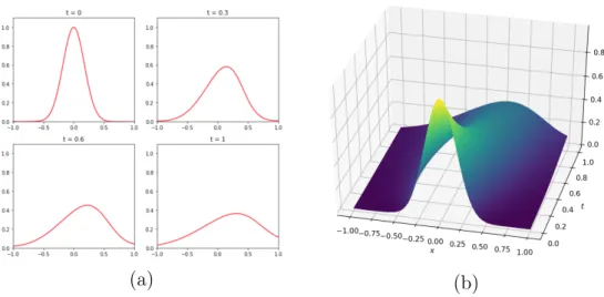
(a) NN(red) and exact(blue) solutions _{(b) NN solution} Figure 3.1: 1D and 3D representations of solution

separation of variables on the boundary condition problem, from which we get two ordinary di↵erential equations (ODE’s) on t and x. From the product of the solution of these two ODE’s we get a family of solutions:

un(x, t) = Bnsin ⇣n⇡x L ⌘ e k(n⇡L) 2 t _{n = 1, 2, 3, . . .}

(30)

20 Chapter 3. Numerical Examples

Finally, when an initial condition is considered, the exact solution is found by setting the free parameters from the boundary condition properly. For example, for ↵ = 1, L = 1 and f (x) = sin(⇡x), we obtain

u(x, t) = sin (⇡x) e k⇡2t,

by choosing n = 1 and B1 = 1. Figures (3.1(a)) and (3.1(b)) shows the solution, for

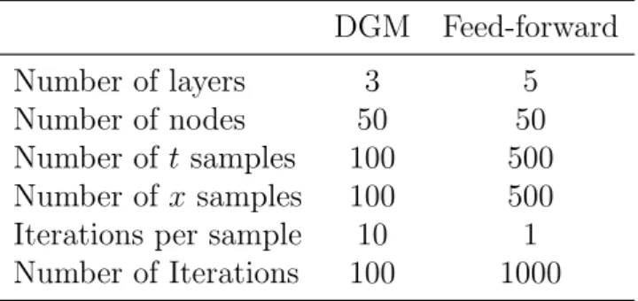
four points in time, of the neural network (in red) against this exact solution. The table below summarizes the training parameters for each architecture

Table 3.1: Training Hyperparameters for the Heat Equation

DGM Feed-forward Number of layers 3 5 Number of nodes 50 50 Number of t samples 100 500 Number of x samples 100 500 Iterations per sample 10 1 Number of Iterations 100 1000

At time t = 0 the temperature is as its peak (i.e. equals 1) at the central point of the x axis. As time passes it gradually spreads and decreases to zero over the whole x axis at around time t = 0.5.

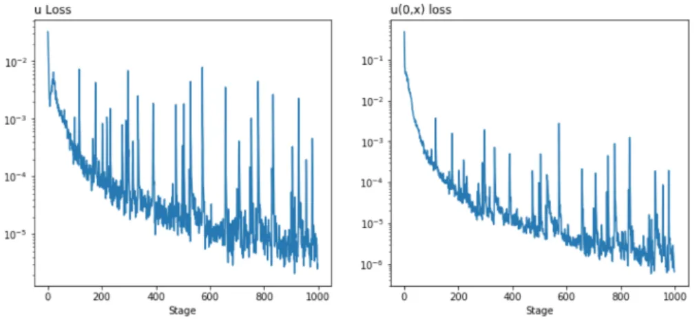
Figure 3.2: Heat Equation Training Loss

(31)

ar-3.3. Burgers Equation 21

chitecture. As it will be seen in other models, although the losses are still decreasing at the end of the iterations, the resulting solution is already satisfactory.

3.3 Burgers Equation

The Burgers equation is one of the fundamental PDE’s, which was originally thought as a way to describe turbulence, as a simplified form of the Navier-Stokes. In fact, it occurs in various fields studying shock waves, fluid dynamics and traffic flow. In its general form it is written as

@tu + u@xu = ⌫@xxu.

The term ⌫ 0 is called the kinematic viscosity. When this term is non-zero, we have the viscid Burgers equation, whereas when it is zero we have the inviscid form of the equation. ₈ > < > : @tu + u@xu = 0, x2 R, t > 0, u(x, 0) = h(x), x2 R. (3.4)

The inviscid form constitutes a non-linear parabolic PDE, one of the simplest equa-tions presenting propagation and di↵usive e↵ects. Figure (3.3) shows the NN solu-tions using the DGM architecture for initial condition g(x) = e x2

. The table below summarizes the training parameters. The solution follows closely other numerical

Table 3.2: Training Hyperparameters for the Inviscid Burgers Equation

DGM Number of layers 3 Number of nodes 50 Number of t samples 500 Number of x samples 500 Iterations per sample 10 Number of Iterations 1000

(32)

(a) _(b)

Figure 3.3: 1D and 3D representations of solution

Figure 3.4: Inviscid Burgers Loss

solutions, which is the usual form to obtain a solution without explicitly considering the phenomenon called wavebreaking, in which past a certain point the peak of the wave moves faster, creating a multiple valued solution. Figure (3.3) shows the loss function for the training of the problem using the DGM architecture. It falls sharply right at the first iterations, and stops improving after around 200 iterations. For the viscid form we will consider the initial-value problem

8 > < > : @tu + u@xu = ⌫@xxu, x 2 R, t > 0, u(x, 0) = h(x), x_{2 R.} (3.5)

(33)

3.4. Buckley-Leverett Equation 23

(a) _(b)

Figure 3.5: 1D and 3D representations of solution

constant ⌫ = 0.1, Figure (3.3) shows the NN solution of the viscid problem. Table (3.3) sumarizes training parameters. Figure (3.3) shows the loss function for the

Table 3.3: Training Hyperparameters for the Viscid Burgers Equation

DGM Number of layers 3 Number of nodes 50 Number of t samples 500 Number of x samples 500 Iterations per sample 10 Number of Iterations 1000

training of the problem using the DGM architecture, which presents a very di↵erent behavior. It continues decreasing after iteration 200, but starts flattening around iteration 900. This might indicate the viscid problem is a harder problem for the NN to learn the solution.

3.4 Buckley-Leverett Equation

A well known problem in the Oil & Gas industry is the analysis of flow of oil in rocks undersea, a problem formally known as the two-phase flow in porous media. Though the equations describing the flow are known, their solution can be quiet

(34)

Figure 3.6: Viscid Burgers Training Loss

expensive in computational terms due to non-linearity and discontinuities. In fact, they may not even me solvable using traditional methods, such as finite di↵erences.

As mentioned previously, in this section we assume a two-phase flow, where each phase corresponds to a distinguishable fluid (i.e. one being water and the other oil). Moreover, under a permeable medium, it is usual to assume that the rate of flow is directly proportional to the drop in vertical elevation between two places in the medium and indirectly proportional to the distance between them, a result known as Darcy’s law.

We also assume both rock and fluid are in-compressible, no geochemical or mechani-cal e↵ects, uniform and isotropic properties and finally that there’s no mass transfer or any volumetric sources.

The equations for imiscible flow can then be written as:

r · qt = 0,

@S

@t +r · qw = 0,

where qt stands for the combined flow of the phases (qt = qw + q0), S stands for

the saturation of the wetting phase (water), and stands for the porosity of the medium. For the one dimensional case, assuming symmetry, we can write the first

(35)

3.4. Buckley-Leverett Equation 25

of the previous equation as @qt

@t = 0, and the flow equation gives rise to the boundary

problem: ₈ > > > > > < > > > > > : @S @t + @F (S) @x = 0, t > 0, x2 (0, 1), S(0, t) = h(t), t 0 S(x, 0) = g(x) x 0. (3.6)

where F is a non-linear function of saturation, and h(t) and g(x) are real functions, indicating the level of water at the beginning and the end of the porous media, respectively. Both are usually set as constants. Moreover,

F (S) = w(S)

w(S) + 0(S)

. (3.7)

where wand 0are called “petrochemical functions”, defined as w(S) = krwmaxSnw/µw

and o(S) = kromax(1 S) no

/µo. Values for these functions are usually obtained

through laboratory measurement, for which typical values are nw = no = 2, krwmax =

kmax

ro = 1, µw = 1⇥ 10 3 and µo = 1.5⇥ 10 3.

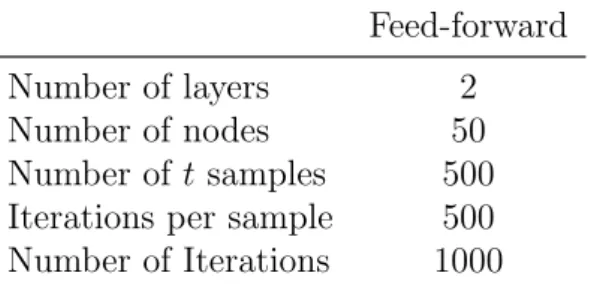
Table 3.4: Training Hyperparameters for the Buckley-Leverett Equation

Feed-forward Number of layers 2 Number of nodes 50 Number of t samples 500 Iterations per sample 500 Number of Iterations 1000

The loss function J for this problem at epoch i is defined as

J(fi) = K X j (@tfi(tj, xj) + @xF (fi(tj, xj)))2 + (fi(t0, xj) h(xj))2+ (fi(tj, x0) g(tj))2

(36)

(a) NN(red) and exact(blue) solutions

(b) NN solution

Figure 3.7: 1D and 3D representation of solutions

Buckley-Leverett equation in one dimension for initial conditions h(t) = 1 and g(x) = 0. The curves represents the water saturation midway through the given medium. The NN solutions falls short when compared to the exact solution, being unable to capture the sharp turn representing the point in which water first touches the medium. The whole dynamic can be seen in the three-dimensional plot in Figure (3.4).

Nonetheless, unlike the other two solutions shown, the DGM results do not approx-imate as well as the feed-forward one. Figure (3.4) shows the cross-sectional plots. The main problem with the solution is that it does not preserve the physical aspect in which there can be no water in points in which it hasn’t arrived yet. For example, in t = 0 there is water-oil saturation across the whole medium, which could only be possible if the liquid spread instantly.

Figure (3.4) shows the loss function for the Buckley-Leverett equation training using the DGM architecture. In line with the poor solutions, the losses seem to stagnate real quick with high variability until the end of the iterations.

(37)

3.5. Mean-Field Games 27

Figure 3.8: Buckley-Leverett solution using the DGM architecture

Figure 3.9: Buckley-Leverett Training Loss

3.5 Mean-Field Games

Mean-field games (MFG’s) are a branch of game theory that studies the strategic interaction of a large number of players, where, usually, the actions of a single player are negligible.The framework as it is presented in this work was first presented in Lachapelle et al. [2016]. A typical mean-field game can be describe as the following

(38)

system (from Cardaliaguet [2010]): 8 > > > > > < > > > > > : (i) @tu ⌫ u + H(x, m, Du) = 0 inRd⇥ (0, T )

(ii) @tm ⌫ m div (DpH(x, m, Du)m) = 0 inRd⇥ (0, T )

(iii) m(0) = m0, u(x, T ) = G(x, m(T ))

where ⌫ is a positive parameter.

The first equation (i) is a Hamilton-Jacobi-Bellman equation, describing the value function of the average small player, while (ii), usually a Fokker-Plank equation, describes the aggregated dynamics of all players.

3.5.1 Optimial Execution with Trade Crowding

In this MFG setup we consider the problem presented in Cardaliaguet and Lehalle [2016] an investor with an initial quantity x to trade, which can be positive or negative depending on whether he wants to sell or boy, respectively. This trade follows a speed ⌫t. The investor is also submitted to risk aversions parameters

and A, which are totally independent of anything else.

Moreover, the trader state following strategy ⌫ is described by its inventory Q⌫

t and

wealth X⌫

t. The evolution of Q⌫ follows

dQ⌫t = ⌫tdt with Q⌫0 = .

He has to finish his trade up to terminal time T .

The tradable instrument has price St, which is described by the equation

(39)

where µt is the net sum of the trading speed of all investors, and Wt is a standard

Wiener process representing an exogenous innovation.

This equation allows us to describe the evolution of a trader wealth

dX_t⌫ = ⌫t(St+ · ⌫t) dt (3.9)

where  is a factor by which wealth is a↵ected by linear trading costs.

Finally we have the cost function. It is made of the wealth at T , plus the value of the inventory penalized by a terminal market impact, and minus a running cost quadratic in the inventory:

Vt := sup ⌫ E ✓ X_T⌫ + Q⌫_T (ST A· Q⌫T) Z T t (Q⌫_s)2ds ◆ . (3.10)

This leads to a Hamilton-Jacobi-Bellman equation, in which since there is an infini-tude of players are considered, their collective dynamics is described by a distribution m.

The full system consisting of a backward PDE on v and a forward transport equation

of m is ₈ > > > > > > > < > > > > > > > : ↵qµt= @tv q2+ (@qv)2 4 , 0 = @tm + @q ✓ m@qv 2 ◆ , µt= Z _@ qv(t, q) 2 m(t, q)dq. (3.11)

with initial conditions m(0, q) = m0(q) and v(T, q; µ) = Aq2.

The DGM approach to solve this system follows the logic employed in the previous problems, with the exception that there is now now more than one PDE of which the loss function will consist, and the integral term for µt.

(40)

a multi-output NN or combine the di↵erent NN’s into one single loss function. The downside of either approach might come in the increase of the number of parameters of time of training. Nonetheless, at least for this specific problem there was no relevant, systematic, change in the training time, even when considering di↵erent number of parameters for the two architectures.

The integral issue is a bit more complex to solve. Since this is a numerical exercise, we need to compute di↵erent points in the domain of the function to be integrated, as in most numerical methods. The problem in this case is that, since the integral considers the time domain, there is the need to compute values of the NN di↵erent from those of a current training, which turns out to be computationally extensive since it implies, for the time indexing, that a di↵erent NN function is considered in each time.

The first approach tried was to compute values for the integral considering only the current epoch NN approximation, although this approach did not fail completely, the loss would stabilize before the values for the m could behave according to the expected behavior.

This led to the implementation of the computation in the fashion of a importance sampling, in which a sample of points in time is set to approximate the integral. Then, each time the integral has to be computed, the current NN approximation is used to sample values to compose the integral.

In practical terms, to guarantee integration to 1 of the resulting equation for m, we first re-write it as m⇤ ₌ e u

c , where c =

R

e u(t,x)_{dx. This change of variable in the}

second equation of (3.11) turns it into

@tu + 1 2k ( @qu@qv + @qqv) + R (@_Rtu) e udx e u_dx = 0 (3.12)

(41)

Then, the resulting integral in (3.12) is approximated by

(tj, xk) = T

X

k=1

@tm (tj, xk) w(xk).

where w (xk) = e u(tj,xk)/PT_k=1e u(tj,xk). While this leads to much better behavior

for m, the number of points in time greatly a↵ects the training time. Finally, the loss function J for this problem at epoch i is defined as

J(fi) = K X j ✓ @tf1,i(tj, xj) + 1

2k( @qf1,i(tj, xj)@qf2,i(tj, xj) + @qqf2,i(tj, xj)) + (tj, xk) ◆2 + K X j ✓ @tf2,i(tj, xj) x2+ @qf2,i(tj, xj)2 4k + ↵xjµ(tj) ◆2 + (f1,i(tj0, xj0) h(xj0)) 2 + (f2,i(tjT, xjT) g(tjT)) 2 . where µ(t) = R

(@qf2,i(t,x))e f1,i(t,x)dq

R

e f1,i(t,x)dq , g(x) = Aq

2 _{and h(x) =} (q c1)2

2c2 , c1 and c2 being

the parameters of a normal distribution.

(a)

NN(red) and exact(blue) solutions (b) NN solution Figure 3.10: Solutions for v and m

Figure (3.10) shows the NN solutions of v and m⇤_{. Table (3.5.1) summarizes the}

training parameters. The behavior of the approximate solution of m⇤ _{follows what}

(42)

increases. The value function v on the other hand is well approximated throughout all time slices, being closest to the real value for small values of q (around 2.5), being overall closest to the analytical solution as the solution reaches time T .

Table 3.5: Training Hyperparameters for the MGF Trade-Crowding problem

DGM

Number of layers 3 Number of nodes 50 Number of t samples 100 Number of x samples 100 Iterations per sample 10 Number of Iterations 500

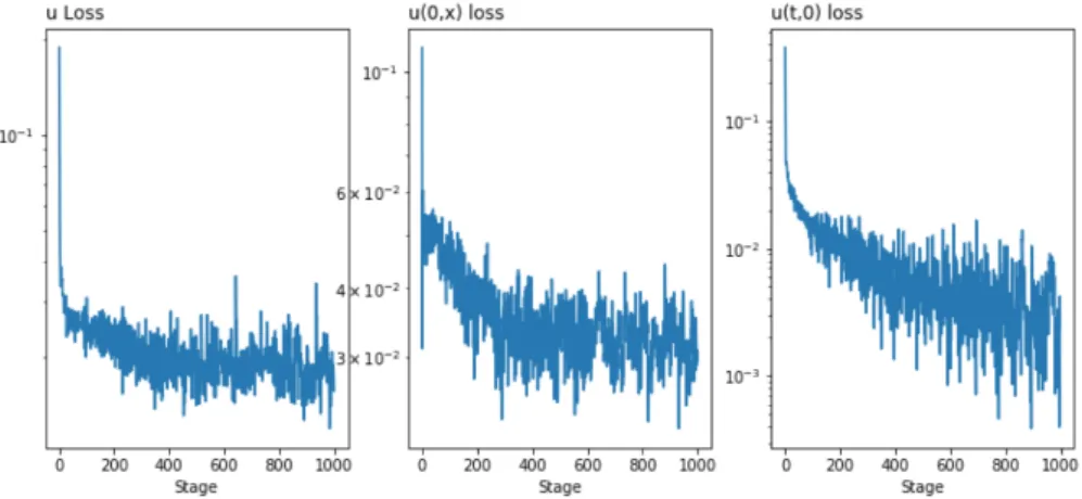
Figure (3.5.1) shows the loss function for the MFG problem of optimal execution with trade crowing. Even tough the losses are still decreasing at the end of 500 iterations, the high computational level of the integral term in the loss function make it a hours-long model to train. Nonetheless, with this number iterations the model already presents really satisfying results, as shown.

(43)

Chapter 4 Conclusion

In this work we investigated the use of neural networks (NN) in approximating the solution of classical PDE’s and more complex controls problems arising in mean-field games.

We used two archtectures, one being a standard feed-forward neural network and the other the DGM method from Sirignano and Spiliopoulos [2017]. Both archi-tectures produced reasonable results, with the DGM yielding the best results in most application, with the exception of the Buckley-Leverett equation, for which the approximation failed to produce physical coherent results.

All the implementations were done using TensorFlow and used only CPU’s. In spite being trained using a personal use computer (MacBook Pro 2015, Core i5 2.7Ghz) most trainings did not require more than minutes to achieve reasonable loses, or even being stopped by a default criteria by TensorFlow’s optimizer, in the case for the feed-forward neural networks.

(44)

Bibliography

Ali Al-Aradi, Adolfo Correia, Danilo Nai↵, Gabriel Jardim, and Yuri Saporito. Solv-ing nonlinear and high-dimensional partial di↵erential equations via deep learnSolv-ing. arXiv preprint arXiv:1811.08782, 2018.

Nicolas Baradel, Bruno Bouchard, and Ngoc Minh Dang. Optimal trading with online parameter revisions. Market Microstructure and Liquidity, page 1750003, 2016.

P. Cardaliaguet. Notes on Mean Field Games: from P.-L. Lions’ lectures at Coll`ege de France. Lecture Notes given at Tor Vergata, 2010.

Pierre Cardaliaguet and Charles-Albert Lehalle. Mean field game of controls and an application to trade crowding. arXiv preprint arXiv:1610.09904, 2016.

Maureen Caudill. Neural networks primer, part i. AI expert, 2(12):46–52, 1987.

G. Cybenko. Approximation by superpositions of a sigmoidal function. Mathematics of Control, Signals, and Systems, 2(4):303–314, December 1989. ISSN 0932-4194, 1435-568X. doi: 10.1007/BF02551274. URL http://link.springer.com/10. 1007/BF02551274.

Ian Goodfellow, Yoshua Bengio, and Aaron Courville. Deep Learning. MIT Press, 2016. http://www.deeplearningbook.org.

(45)

BIBLIOGRAPHY 35

Jiequn Han, Arnulf Jentzen, and E. Weinan. Solving high-dimensional partial dif-ferential equations using deep learning. arXiv:1707.02568 [cs, math], July 2017. URL http://arxiv.org/abs/1707.02568. arXiv: 1707.02568.

Sepp Hochreiter and J¨urgen Schmidhuber. Long short-term memory. Neural Computation, 9(8):1735–1780, 1997. doi: 10.1162/neco.1997.9.8.1735. URL https://doi.org/10.1162/neco.1997.9.8.1735.

Kurt Hornik. Approximation capabilities of multilayer feedforward networks. Neural networks, 4(2):251–257, 1991.

Aim´e Lachapelle, Jean-Michel Lasry, Charles-Albert Lehalle, and Pierre-Louis Lions. Efficiency of the price formation process in presence of high frequency participants: a mean field game analysis. Math. Financ. Econ., 10(3):223–262, 2016. ISSN 1862-9679. doi: 10.1007/s11579-015-0157-1. URL http://dx.doi.org/10.1007/ s11579-015-0157-1.

I. E. Lagaris, A. Likas, and D. I. Fotiadis. Artificial Neural Networks for Solving Ordinary and Partial Di↵erential Equations. IEEE Transactions on Neural Net-works, 9(5):987–1000, September 1998. ISSN 10459227. doi: 10.1109/72.712178. URL http://arxiv.org/abs/physics/9705023. arXiv: physics/9705023.

Hyuk Lee and In Seok Kang. Neural algorithm for solving di↵erential equa-tions. Journal of Computational Physics, 91(1):110–131, November 1990. ISSN 00219991. doi: 10.1016/0021-9991(90)90007-N. URL http://linkinghub. elsevier.com/retrieve/pii/002199919090007N.

Christopher Olah. Understanding lstm networks, 2015. URL http://colah. github.io/posts/2015-08-Understanding-LSTMs/.

Daniel R Parisi, Maria C Mariani, and Miguel A Laborde. Solving di↵erential equations with unsupervised neural networks. Chemical Engineering and Pro-cessing: Process Intensification, 42(8-9):715–721, August 2003. ISSN 02552701.

(46)

36 BIBLIOGRAPHY

doi: 10.1016/S0255-2701(02)00207-6. URL http://linkinghub.elsevier.com/ retrieve/pii/S0255270102002076.

Maziar Raissi, Paris Perdikaris, and George Em Karniadakis. Physics Informed Deep Learning (Part I): Data-driven Solutions of Nonlinear Partial Di↵erential Equations. arXiv:1711.10561 [cs, math, stat], November 2017. URL http:// arxiv.org/abs/1711.10561. arXiv: 1711.10561.

Justin Sirignano and Konstantinos Spiliopoulos. DGM: A deep learning algorithm for solving partial di↵erential equations. arXiv:1708.07469 [math, q-fin, stat], August 2017. URL http://arxiv.org/abs/1708.07469. arXiv: 1708.07469.