ISSN 0104-6632 Printed in Brazil
www.abeq.org.br/bjche
Vol. 33, No. 02, pp. 347 - 360, April - June, 2016 dx.doi.org/10.1590/0104-6632.20160332s20150011
*To whom correspondence should be addressed
Brazilian Journal
of Chemical
Engineering
3D COMPOSITIONAL RESERVOIR
SIMULATION IN CONJUNCTION WITH
UNSTRUCTURED GRIDS
A. L. S. Araújo
1, B. R. B. Fernandes
2, E. P. Drumond Filho
2, R. M. Araujo
2,
I. C. M. Lima
2, A. D. R. Gonçalves
2, F. Marcondes
3*and K. Sepehrnoori
41
Federal Institute of Education, Science and Technology of Ceará, Fortaleza - CE, Brazil. 2
Laboratory of Computational Fluid Dynamics, Federal University of Ceará, Fortaleza - CE, Brazil. 3
Department of Metallurgy and Materials Science and Engineering, Federal University of Ceará, Fortaleza - CE, Brazil.
*
E-mail: [email protected] 4
Center for Petroleum and Geosystems Engineering, The University of Texas at Austin, USA. (Submitted: January 7, 2015 ; Revised: April 6, 2015 ; Accepted: May 24, 2015)
Abstract - In the last decade, unstructured grids have been a very important step in the development of petroleum reservoir simulators. In fact, the so-called third generation simulators are based on Perpendicular Bisection (PEBI) unstructured grids. Nevertheless, the use of PEBI grids is not very general when full anisotropic reservoirs are modeled. Another possibility is the use of the Element based Finite Volume Method (EbFVM). This approach has been tested for several reservoir types and in principle has no limitation in application. In this paper, we implement this approach in an in-house simulator called UTCOMP using four element types: hexahedron, tetrahedron, prism, and pyramid. UTCOMP is a compositional, multiphase/multi-component simulator based on an Implicit Pressure Explicit Composition (IMPEC) approach designed to handle several hydrocarbon recovery processes. All properties, except permeability and porosity, are evaluated in each grid vertex. In this work, four case studies were selected to evaluate the implementation, two of them involving irregular geometries. Results are shown in terms of oil and gas rates and saturated gas field.
Keywords: EbFVM; Compositional reservoir simulation; IMPEC approach; Unstructured grids.
INTRODUCTION
Proper petroleum reservoir modeling requires the correct evaluation of several important geometric pa-rameters, such as sealing faults, fractures, irregular reservoir shapes, and deviated wells. Although sim-ple to use, conventional Cartesian grids, commonly employed in petroleum reservoir simulation, cannot produce accurate modeling of most of the aforemen-tioned geometric features. The first application of unstructured grids in the petroleum reservoir area were carried out by Forsyth (1990), Fung et al. (1991), and Gottardi et al. (1992). The
348 A. L. S. Araújo, B. R. B. Fernandes, E. P. Drumond Filho, R. M. Araujo, I. C. M. Lima, A. D. R. Gonçalves, F. Marcondes and K. Sepehrnoori
Brazilian Journal of Chemical Engineering
approach is the necessity to solve a local linear sys-tem in order to maintain the flux continuity. This issue is raised by the storage of permeability in each vertex of the grid. Using the Element based Finite-Volume Method (EbFVM), as presented in this pa-per, and storing a permeability tensor for each ele-ment overcomes this problem. Furthermore, fully heterogeneous and anisotropic reservoirs can also be handled using this approach.
Several studies have been conducted in order to further develop and enhance the CVFEM method. Cordazzo (2004) and Cordazzo et al. (2004) applied the ideas of Raw (1985) and Baliga and Patankar (1983) to simulate waterflooding problems. Concern-ing the final governConcern-ing equations, this method is very similar to the CVFEM. The resulting approach was called the Element-based Finite Volume Method (EbFVM), which is a more suitable denomination, since it borrows the flexibility of the finite-element method to discretize the domain, but keeps the con-servative idea from the finite-volume method. The main difference between the CVFEM approach com-monly used in petroleum reservoir simulation and the EbFVM technique lies in the assumption of mul-tiphase/multi-component flow of the EbFVM ap-proach in order to obtain the approximate equations, while the CVFEM first obtains the approximate equa-tions for single phase flow and then multiplies the re-sulting equations by the mobilities in order to obtain the approximate equations for multiphase flow. Later, Paluszny et al. (2007) presented a full tridimensional discretization for hexahedron, tetrahedron, prism, and pyramid elements in conjunction with water flooding problems. Marcondes and Sepehrnoori (2010) and Marcondes et al. (2013) applied the EbFVM to 2D and 3D isothermal, compositional problems using a fully implicit approach. Santos et al. (2013) applied the EbFVM to the solution of 3D compositional mis-cible gas flooding with dispersion, once again associ-ated with the fully implicit approach. These works demonstrated that more accurate solutions can be obtained with the EbFVM compared to Cartesian grids. Fernandes et al. (2013) investigated several interpolation functions for the solution of composi-tional problems for 2D reservoirs in conjunction with the EbFVM approach. Marcondes et al. (2015) im-plemented EbFVM to 2D and 3D thermal, composi-tional reservoir simulator in conjunction with a fully implicit approach.
This work presents an investigation of the EbFVM method for the solution of isothermal, multicompo-nent/multiphase flows in 3D reservoirs using four element types: hexahedron, tetrahedron, prism and pyramid in conjunction with an IMPEC (Implicit
Pressure Explicit Composition) approach. The poros-ity and permeabilporos-ity tensors are constant throughout each element. All remaining properties are evaluated at the vertices of each element, defining a cell-vertex approach. The method was implemented in the UTCOMP simulator, developed at the Center of Pe-troleum and Geosystems Engineering at The Univer-sity of Texas at Austin for handling several composi-tional, multiphase/multicomponent recovery pro-cesses. To the best of our knowledge, this is the first time that the EbFVM in conjunction with hexahe-drons, tetrahehexahe-drons, prisms, and pyramids is imple-mented and tested for compositional reservoir simu-lation based on an IMPEC approach.
GOVERNING EQUATIONS
According to Wang et al. (1997), in order to de-scribe an isothermal, multiphase/multicomponent flow in a porous medium, three types of equations are required: the material balance for all components, the phase equilibrium equations, and the equations for constraining phase saturations and component con-centrations.
The material balance equation for each compo-nent is given by
1
1
0
for 1, 2, ,
p
n
i i
j j ij j
b j b
c
N q
x k
V t V
i n
ξ λ =
∂ − ∇⋅ ⎡ ⋅∇Φ −⎤ =
⎣ ⎦
∂ =
∑
G G
" , (1)
where Ni is the number of moles of the i-th
compo-nent, ξj, λj are respectively, the molar density and
molar mobility of the j-th phase, xij is the mole
frac-tion of the i-th component in the j-th phase, qi is the
molar rate of the i-th component, Vb is bulk volume,
k is the absolute permeability tensor, and Φj is the
phase potential of the j-th phase which is given by
j Pj γjD Pcjr
Φ = − + , (2)
where Pj is the pressure of the j-th phase, Pcjr
repre-sents the capillary pressure between phases j and r, γj
is the specific gravity of the j-th phase, and D is the reservoir depth which is positive in the downward direction. In UTCOMP, the oil phase is the reference phase.
3D Compositional Reservoir Simulation in Conjunction with Unstructured Grids 349
Brazilian Journal of Chemical Engineering Vol. 33, No. 02, pp. 347 - 360, April - June, 2016 number and composition of all phases, satisfying
three conditions. First, the molar-balance equation has to be considered. Next, the chemical potentials for each component must be the same for every phase. The last condition is the minimization of the Gibbs free energy. The first partial derivate of the total Gibbs free energy for the independent variables results in the equality of all component fugacities throughout all phases, which can be stated, consider-ing oil as the reference phase (r), as
0 ( 1, 2, , ; 3, , ; 2).
j r
i i c p
f − f = i= " n j= " n r= (3)
Note that the water phase is not included in the phase equilibrium calculations.
The phase composition constraints and the equa-tion for determining the phase amounts for both hy-drocarbon phases are, respectively, given by
1
1 0 ( 1, 2, , ),
c
n
ij p
i
x j n
=
− = =
∑
" (4)(
)
(
)
1
1 0.
1 1
c
n
i i
i i
z K
v K
=
− =
+ −
∑
(5)In Eq. (5), Ki stands for the equilibrium ratio for each component, zi is the overall mole fraction, and v
represents the gas mole fraction in the absence of water.
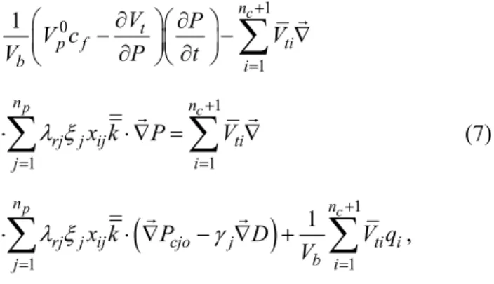
The last equation to be obtained is the pressure equation. The UTCOMP simulator is based on an IMPEC (Implicit Pressure, Explicit Composition) approach. In this formulation, the pressure is solved implicitly, while the conservations, Equation (1), are evaluated explicitly. In each grid block, the pressure is obtained from the assumption that the pore volume is completely filled with the total volume of fluid
( , ) ( ),
t p
V P NG =V P (6)
where the pore volume (Vp) is a function only of the
pressure, while the total fluid volume (Vt) is a
func-tion of pressure and the total number of moles of each component. Differentiating each side of Eq. (6) with respect to their independent variables, the pres-sure equation (Ács et al., 1985; Chang, 1990) is ob-tained as follows:
(
)
1 0
1
1
1 1
1
1 1
1
1
,
c
p c
p c
n t
p f ti
b i
n n
rj j ij ti
j i
n n
rj j ij cjo j ti i
b
j i
V P
V c V
V P t
x k P V
x k P D V q
V
λ ξ
λ ξ γ
+ = +
= =
+
= =
∂ ∂
⎛ − ⎞⎛ ⎞− ∇
⎜ ⎟ ⎜ ∂ ⎟⎝ ∂ ⎠
⎝ ⎠
⋅ ⋅∇ = ∇
⋅ ⋅ ∇ − ∇ +
∑
∑
∑
∑
∑
G
G G
G G
(7)
where Vti represents the derivative of total fluid volume related to Ni.
APROXIMATE EQUATIONS
The EbFVM method is characterized by dividing each element into sub-elements according to the number of vertices. Conservation equations, Eqs. (1) and (7), are integrated over each sub-element. After the division of the elements into sub-elements, we call them sub-control volumes. The material balance is established for every sub-control volume, and then, the control volume balance equation is built by adding the contributions of every sub-control volume that shares the same vertex.
Each element type has a certain sub-control volume division based on the number of vertices. Figure 1 shows the division for each of the four ele-ments investigated in this work, according to the number of vertices. From Figure 1, it is possible to infer that each sub-control volume for hexahedron, prism, and tetrahedron elements is composed of three quadrilateral integration surfaces. The exception is the pyramid element, whose sub-control volumes associated with the base have three triangular in-tegration surfaces and the one associated with the apex has four quadrilateral integration surfaces. In Figure 1, the numbers that reside inside a circle refer to the integration surface and the others refer to the vertices.
Integrating Eq. (1) in time and over each sub-con-trol volume, followed by the application of the Gauss theorem for the advective term, we obtain:
1
, ,
1 ,
1
0 ; 1, 2,.., .
p
n i
j ij j j
b j
V t A t i
c b
V t
N
dVdt x k dAdt
V t
q
dVdt i n
V
ξ λ
= +
∂ − ⋅∇Φ ⋅
∂
− = =
∑
∫
∫
∫
G G
35 in ti h m N N N N N N N N N N
50 A. L. S. A
In order to n Eq. (8), it ions for each exahedron, ments are, res
1 2 3 4 5 6 7 8 (1 ( , , ) ( ( , , ) (1 ( , , ) ( ( , , ) ( ( , , ) ( ( , , ) ( ( , , ) (1 ( , , ) N s t p
N s t p
N s t p
N s t p
N s t p
N s t p
N s t p
N s t p
= = = = = = = = 1 3
( , , ) 1
( , , )
N s t p
N s t p t = =
Araújo, B. R. B. F
Figure
(b) tetra
o evaluate the is necessary h element typ tetrahedron, spectively, de
1 )(1 )(1 8 1 )(1 )(1
8 1 )(1 )(1
8 1 )(1 )(1
8 1 )(1 )(1
8 1 )(1 )(1
8 1 )(1 )(1
8 1 s t s t s t s t s t s t s t s + − + − − − − − + + + + − +
− )(1 )(1 8 t + 4 1 ; ; ( , ,
s t p
t N s t p − − −
Fernandes, E. P. D
(a)
(c)
1: Sub-cont ahedron, (c) p
e volume, ar y to define t pe. The shap prism, and efined as foll
) ; ) ) ; ) ) ; ) ) ; p p p p p p p + − − + + − − ) , p + 2 ; ( , , ) ) ,
N s t p
p =p
Drumond Filho, R
Brazilian Jou
)
)
trol volumes prism, and (d
rea and gradi the shape fu pe functions d pyramid e
lows:
s =
(1
R. M. Araujo, I. C
urnal of Chemica
for the four d) pyramid (M
ient unc-for ele-(9) 10) 1 3 5 N N N 1 3 N N N N N s, fra all of z s ev ins par
C. M. Lima, A. D
al Engineering
(
( r element typ Marcondes e
1
3
5
( , , ) (1
( , , ) (1
( , , ) s t p
s t p t
s t p sp
= − = = 1 2 3 4 5 1 ( , , ) [ 4 1 ( , , ) 4 1 ( , , ) [ 4 1 ( , , ) 4 ( , , ) N s t p
N s t p
N s t p
N s t p
N s t p p
=
=
=
= =
In the shap t, and p are ame, defined lows all elem
how distorte system. Sinc aluate any p side each ele
rametric elem
. R. Gonçalves, F
(b)
(d)
pes: (a) hexa et al., 2015).
4
6
)(1 )
) ; ( ,
; ( , , )
s t p
p N s
N s t p
− − − −
[(1 )(1 )
[(1 )(1 )
[(1 )(1 )
[(1 )(1 )
. s t s t s t s t − − + − + + − +
e function e e the coordin d in each e ments to be t
ed an elemen ce we emplo physical prop ement, these ments (Hugh
F. Marcondes and
ahedron,
2
) ; ( , , )
, ) (1
) ,
N s t p
t p p s
tp
= − =
/ (1
) / (
) / (1
) / (1
p stp p stp p stp p stp − + − − − − − − equations pre nates in a l element. Thi treated equa nt is in the g oy the shape perty or geom e elements a hes, 1987):
d K. Sepehrnoori
(1 ) ) s p s t = − − (11 1 )] 1 )] 1 )] 1 )] p p p p − − − − (12 esented abov ocal referen is local fram ally, regardle global x, y, an
e functions metry positio are called is
so-3D Compositional Reservoir Simulation in Conjunction with Unstructured Grids 351
Brazilian Journal of Chemical Engineering Vol. 33, No. 02, pp. 347 - 360, April - June, 2016
1 1
1 1
( , , ) ; ( , , ) ;
( , , ) ; ( , , ) .
Nv Nv
i i i i
i i
Nv Nv
i i j i ji
i i
x s t p N x y s t p N y
z s t p N z s t p N
= =
= =
= =
= Φ = Φ
∑
∑
∑
∑
(13)
In Eq. (13), Nv and Ni denote the number of
verti-ces and the shape functions of each element, respec-tively. From Eq. (13), the gradient of phase potential can be written as
1 1
1
; ;
.
Nv Nv
j i j i j
ji ji i i Nv i ji i N N
x x y y z
N z
= =
=
∂Φ = ∂ Φ ∂Φ = ∂ Φ ∂Φ
∂ ∂ ∂ ∂ ∂ ∂ = Φ ∂
∑
∑
∑
(14)The shape function derivatives required for com-puting the gradients in Eq. (14) are given by:
1 det( ) 1 det( ) 1 det( ) 1 det( ) 1 det( ) 1 de i i t i t i t i i t i t
N y z y z N
x J t p p t s
N
y z y z
J s p p s t
N
y z y z
J s t t s p
N x z x z N
y J t p p t s
N
x z x z
J s p p s t
⎛ ⎞ ∂ = ∂ ∂ ∂ ∂− ∂ ⎜ ⎟ ∂ ⎝ ∂ ∂ ∂ ∂ ⎠ ∂ ⎛ ∂ ∂ ∂ ∂ ⎞ ∂ − ⎜ − ⎟ ∂ ∂ ∂ ∂ ∂ ⎝ ⎠ ∂ ∂ ∂ ∂ ∂ ⎛ ⎞ + ⎜ − ⎟ ∂ ∂ ∂ ∂ ∂ ⎝ ⎠ ⎛ ⎞ ∂ =− ∂ ∂ ∂ ∂− ∂ ⎜ ⎟ ∂ ⎝ ∂ ∂ ∂ ∂ ⎠ ∂ ⎛ ∂ ∂ ∂ ∂ ⎞ ∂ + ⎜ − ⎟ ∂ ∂ ∂ ∂ ∂ ⎝ ⎠ − t( ) 1 det( ) 1 det( ) 1 , det( ) i t i i t i t i t N
x z x z
J s t t s p
N x y x y N
z J t p p t s
N
x y x y
J s p p s t
N
x z x y
J s t t s p
∂ ∂ ∂ ∂ ∂ ⎛ − ⎞ ⎜ ∂ ∂ ∂ ∂ ⎟ ∂ ⎝ ⎠ ⎛ ⎞ ∂ = ∂ ∂ −∂ ∂ ∂ ⎜ ⎟ ∂ ⎝ ∂ ∂ ∂ ∂ ⎠ ∂ ⎛ ∂ ∂ ∂ ∂ ⎞ ∂ − ⎜ − ⎟ ∂ ∂ ∂ ∂ ∂ ⎝ ⎠ ∂ ∂ ∂ ∂ ∂ ⎛ ⎞ + ⎜ − ⎟ ∂ ∂ ∂ ∂ ∂ ⎝ ⎠ (15)
where det(Jt) is the Jacobian of the transformation
and is given for all sub-control volumes by:
det( )
. t
x y z y z
J
s t p p t
x y z y z
t s p p s
x y z y z
p s t t s
⎛ ⎞ ∂ ∂ ∂ ∂ ∂ = ⎜ − ⎟ ∂ ∂ ∂⎝ ∂ ∂ ⎠ ⎛ ⎞ ∂ ∂ ∂ ∂ ∂ − ⎜ − ⎟ ∂ ∂ ∂⎝ ∂ ∂ ⎠ ∂ ∂ ∂ ∂ ∂⎛ ⎞ + ⎜ − ⎟ ∂ ∂ ∂ ∂ ∂⎝ ⎠ (16)
The sub-control volumes for the hexahedron, tetra-hedron, prism, and pyramid elements are given, re-spectively, by Eqs. (17) through (20), and the area for quadrilateral integration surfaces is given by Eq. (21).
, det( )
scv i t
V = J , (17)
, det( ) / 6
scv i t
V = J , (18)
, det( ) / 12
scv i t
V = J , (19)
,
2det( ) / 9 1,..., 4 ( )
4det( ) / 9 5 ( )
t scv i
t
J for i base
V
J for i apex
= ⎧
=⎨ =
⎩ , (20)
ˆ
ˆ
ˆ ,
y z y z
dA dm dn i
m n n m
x z x z
dm dn j
n m m n
x y x y
dm dn k
m n n m
∂ ∂ ∂ ∂ ⎛ ⎞ =⎜ − ⎟ ∂ ∂ ∂ ∂ ⎝ ⎠ ∂ ∂ ∂ ∂ ⎛ ⎞ −⎜ − ⎟ ∂ ∂ ∂ ∂ ⎝ ⎠ ∂ ∂ ∂ ∂ ⎛ ⎞ +⎜ − ⎟ ∂ ∂ ∂ ∂ ⎝ ⎠ G (21)
where m and n in Eq. (21) represent the local system s, t, or p. The computation of the integrated surface area for the remaining element types is similar. Equa-tions (17) - (20) and Eq. (21) are used to evaluate, respectively, the accumulation term (Acc) and the advective flux (F).
,
1 ,
,
;
1, ; 1,.., 1
m i
n n scv m m m i
b m i i v c
V N N
Acc
V t t
m N i n
+ ⎛⎛ ⎞ ⎛ ⎞ ⎞ ⎜ ⎟ = ⎜⎜ ⎟ −⎜ ⎟ ⎟ Δ Δ ⎝ ⎠ ⎝ ⎠ ⎝ ⎠
= = + , (22)
(
)
, 1 3 1 1 ;1, ; , 1,...,3; 1, 1.
p
p
j ij j
n
m i j ij j j j
A n
j n n n
nl n l ip j ip
v c
F x k dA
x k A
x
m N n l i n
ξ λ
ξ λ
=
= =
= ⋅∇Φ ⋅
⎛ ∂Φ ⎞
352 A. L. S. Araújo, B. R. B. Fernandes, E. P. Drumond Filho, R. M. Araujo, I. C. M. Lima, A. D. R. Gonçalves, F. Marcondes and K. Sepehrnoori
Brazilian Journal of Chemical Engineering
From Eq. (23), it is possible to infer that it is nec-essary to calculate molar densities, mole fractions, and molar mobilities at each one of the interfaces of each sub-control volume. Also, it is important to note that the aforementioned properties are evaluated at the previous time step (superscript n); the superscript ‘n+1’ denotes the current time-step. It is also im-portant to indicate that, for the potential term in Eq. (23), only the pressure is evaluated implicitly, while the other terms (capillary pressure and gravitational terms) are evaluated explicitly. In order to evaluate the mentioned properties, an upwind scheme is used. Considering the integration point 1 of Fig 1, for all the elements, the mobility is calculated as:
1 2
1
1 1
1
0
0.
jip j j ip jip j j
ip
if k dA
if k dA
λ λ
λ λ
= ⋅∇Φ ⋅ ≤
= ⋅∇Φ ⋅ >
G G
G
G (24)
Inserting Eqs. (22) and (23) in Eq. (8), the final equation for each sub-control volume is given by
, , 0 ; 1,..., ; 1,..., 1.
m i m i i v c
Acc +F + =q m= N i= n + (25)
Eq. (25) represents the material balance for each sub-control volume. The equations for each control-volume are assembled from the contribution of all sub-control volumes that share the same vertex. Fur-ther details about this procedure can be found in Marcondes and Sepehrnoori (2010) and Marcondes et al. (2013). A similar procedure realized for the molar balance equation needs to be performed for the pressure equation.
RESULTS AND DISCUSSION
In this section, results for four case studies are presented. The two first case studies are designed to validate the current implementation with the Carte-sian implementation of the UTCOMP simulator, and the other two case studies are designed to demon-strate the ability of the EbFVM approach to handle irregular geometries. It is important to emphasize that the Cartesian implementation of UTCOMP simu-lator has been validated using many analytical solu-tions as well as several commercial simulators (Chang, 1990; Fernandes et al., 2013). The first case is a CO2 injection characterized by three hydrocar-bon components in a quarter-of-five-spot configura-tion. The reservoir data, components and composi-tion data, and binary coefficients are shown in Tables
1 through 3, respectively. For all grid configurations investigated in this work, red arrows denote producer wells, while blue arrows denote injecting wells.
Table 1: Reservoir data for Case 1.
Property Value
Length, width, and thickness
170.69 m, 170.69 m, and 30.48 m
Porosity 0.30 Initial Water Saturation 0.25
Initial Pressure 20.65 MPa Permeability in X, Y,
and Z directions
1.974x10⁻¹³ m2, 1.974x10⁻¹³ m2, and 1.974x10⁻¹⁴ m2
Formation Temperature 299.82 K Gas Injection Rate 5.66x10² m3/d Producer’s Bottom
Hole Pressure
20.65 MPa
Table 2: Fluid composition data for Case 1.
Component Initial Reservoir
Composition
Injection Fluid Composition
CO2 0.0100 0.9500
C1 0.1900 0.0500
n-C16 0.8000 -
Table 3: Binary interaction coefficients for Case 1.
The volumetric rates of oil and gas obtained with all the four elements investigated and the refined Cartesian grid are presented in Figure 2. From this figure, it is possible to infer that all four elements produce results that are in good agreement with the ones obtained with the refined Cartesian grid. Also, the number of volumes for all elements used is much smaller than the ones used by the Cartesian grid, demonstrating that, at least for this case study, the EbFVM approach is much more accurate than the Cartesian grid. Accuracy can be explained based on the larger Jacobian stencil of the unstructured grid compared to the convention seven bandwidth diago-nals of the Cartesian grid.
In order to visualize the pyramid mesh, Figure 3 shows a x-y plane cut through the apex of one pyra-mid element.
Figure 4 presents the saturation gas field at 500 days for all elements tested and for the Cartesian grid. From this figure, once again it is possible to conclude that very good sharp fronts were obtained with all elements and these results are in good agree-ment with the refined Cartesian mesh.
Component CO2 C1 n-C16
CO2 - 0.12 0.12
C1 0.12 - -
3
Brazi
3D Compositiona
ilian Journal of C
(a)
Figure 2
Figure 3: A
(a)
(c)
l Reservoir Simu
Chemical Enginee
2: Volumetric
Aerial view o
ulation in Conjunc
ering Vol. 33, No
c rates - Case
of the cut pla
ction with Unstru
o. 02, pp. 347 - 3
e 1: a) Oil an
ane of the pyr
uctured Grids
60, April - June,
(b) nd b) Gas.
ramid mesh.
(b)
(d)
, 2016
35
je ac en se co
te
54 A. L. S. A
Figure 4
Tetrahed
The secon ection proble cterized with nce is that th et to zero, w ompletely m
Figure 5 s esian grid an
Araújo, B. R. B. F
4: Gas satu dron and (e) P
nd case study em in a quart h same fluid he binary int which in tur miscible with shows the co nd the four el
Fernandes, E. P. D
uration at 50 Pyramid.
y again refer ter-of-five sp of case stud teraction coe rn makes the
the oil in-pla omparison be lement types
(a)
Figure 5
(a)
Drumond Filho, R
Brazilian Jou
00 days for
rs to a CO2 pot and is ch dy 1. The diff efficients are
e injected fl ace.
etween the C s, for Case 2
5: Volumetric
R. M. Araujo, I. C
urnal of Chemica
(e) Case 1. (a)
in- har- ffer-e all
luid
Car-, in
ter pre ele
is it tw sia
c rates - Case
C. M. Lima, A. D
al Engineering
) Cartesian;
rms of oil a esented in Fi ements and th
The CO2 ov shown in F is possible ween the EbF
an grid.
e 2: a) Oil an
. R. Gonçalves, F
(b) Hexahe
and gas prod ig. 5 show a he Cartesian verall mole
igure 6. Fro to observe FVM for all
(b) nd b) Gas.
(b)
F. Marcondes and
edron; (c) P
duction rate a satisfactory n grid.
fraction fiel om the resu e a good a l elements a
d K. Sepehrnoori
rism; (d)
s. The resul y match for a
ld at 500 day ults presente
greement b and the Cart
lts all
te-p se re th
F
h
Figure 6
Prism; (d
The third c roblem in a even hydroc eservoir is sh he reservoir
Figure 7: Gr hybrid grid (1
3
Brazi
6: CO2 overa d) Tetrahedro
case study ag an irregular carbon comp hown in Figu
dimensions,
rid configura 19928 vertice
3D Compositiona
ilian Journal of C
(c)
all mole frac on and (e) Py
gain refers to reservoir ch ponents. Th ure 7. Just to , the sizes i
(a) ations used f
es; 14352 tet
l Reservoir Simu
Chemical Enginee
ction fields fo yramid.
o a gas flood haracterized e 3D irregu have an idea n Figure 7
for Case 3. ( trahedrons; 1
ulation in Conjunc
ering Vol. 33, No
(e) for Case 2 at
ding by ular a of are
sho in hex me mi
(a) Hexahedr 12688 hexah
ction with Unstru
o. 02, pp. 347 - 3
t 500 days. (
own in feet. Figure 7; Fig xahedron ele esh composed ids elements.
ron grid (148 edrons; 7800
uctured Grids
60, April - June,
(d)
a) Cartesian;
Two grid co gure 7a show ements, and
d of hexahed
(b) 896 vertices; 0 pyramids).
, 2016
; (b) Hexahe
onfigurations ws a grid com
Figure 7b sh dron, tetrahed
)
; 12987 elem
3
edron; (c)
s are presente mposed of on
hows a hybr dron, and pyr
ments) and (b
355
ed nly rid
35
in
56 A. L. S. A
The reserv n Tables 4 an
Table Proper Porosity Initial Water Initial Pressur Permeability and Z directio Formation Te Gas Injection Producer’s Bo Hole Pressure
Table 5: F
Component
CO2 C1 C2-C3 C4-C6 C7-C14 C15-C24 C25+ Figure 8 s
Araújo, B. R. B. F
voir and fluid nd 5, respecti
e 4: Reservo
rty
Saturation re
in X, Y, ons emperature n Rate ottom e Fluid compo
t Initial R
Comp 0.0 0.2 0.1 0.1 0.2 4 0.1 0.0 shows the to
Fernandes, E. P. D
d composition ively.
oir data for C
Va
0.163 0.25 19.65 MPa 1.974x10⁻¹³ m2 and 1.974x10 -400 K 14.16x10³ m3/ 19.65 MPa osition data Reservoir position 0077 2025 1180 1484 2863 1490 0881
otal oil and
(a)
Figure 8:
(a)
Drumond Filho, R
Brazilian Jou
n data are giv
Case 3.
alue
2
, 1.974x10⁻¹³ m 14
m2 d
for Case 3.
Injection Fluid Composition 0.96 0.01 0.01 0.01 0.01 - - gas volumet
: Volumetric
R. M. Araujo, I. C
urnal of Chemica
ven
m2,
d tric rat wi he fig the fig sim the Al dif pre go sio ga co sen hy me ter fro ics sia cel ad
rates for Ca
C. M. Lima, A. D
al Engineering
tes from the ith the hexah
dron and pri gure, it is pos e results obta gurations.
Figure 9 pr mulated time e hexahedron lthough, the fferent from esented in F ood resolutio
on were obse The fourth s) injection mponents in nts two grid ybrid grid. Ju
ensions, the rms of the g om Case 3, si s a region of an mesh is u
lls should be ditional calc
se 3. a) Oil a
. R. Gonçalves, F
two produce hedron and h ism elements ssible to see a ained with th
resents the g es (100 days
n and hybrid grid confi each other, Fig. 9 are i n fronts wit erved.
case study is characteriz n a 3D irreg d configurat ust to have a sizes in Fig geometric mo
ince there is f small perm used to mod e used. Using ulation is ne
(b) and b) Gas
(b)
F. Marcondes and
ers obtained hybrid (hexa s) refined gr a good agree the two diffe
gas saturatio s; 280 days) d grids show igurations ar , the gas sat in good agr th small num
s a mixed flu zed by five gular grid. F
tions: a hex an idea of th g. 10 are sho odel, this ca an internal h meability tens
del such an g the EbFVM ecessary.
d K. Sepehrnoori
in conjunctio ahedron, tetr rids. From th ement betwee erent grid co
n field at tw obtained wi wn in Figure re complete turation fiel reement. Als merical dispe
uid (liquid an e hydrocarbo Figure 10 pr xagonal and
e reservoir d own in feet. ase is differe hole that mim sor. If a Cart
ar
ju th b
Figure 9
d) 280 d
Figure 1
and (b) h
The reserv re shown in T
Figure 11 unction with his figure, is etween the tw
Table
Pro
Porosity Initial Wate Initial Pres Permeabilit directions Formation Gas Injecti Producer’s Hole Pressu
3
Brazi
9: Gas satura days.
10: Grid con hybrid grid (4
voir and flui Tables 6 and presents the the hexahed possible to wo grid conf
e 6: Reservo
operty
er Saturation sure ty in all Temperature on Rate
Bottom ure
3D Compositiona
ilian Journal of C
(c) ation fields fo
(a) figurations u 42232 vertic
id compositi d Table 7, res e oil and ga dron and hyb observe a ve figurations in
oir data for C
0.3 0.1 10. 9.8 344 28. 8.9
l Reservoir Simu
Chemical Enginee
or Case 3. H
used for Case ces; 4200 tetr
ion informat spectively. as rates in c brid grids. Fr ery good ma nvestigated.
Case 4.
Value
35 7 .34 MPa 869x10-15m2
4.26 K .32x103 m3/d 96 MPa
ulation in Conjunc
ering Vol. 33, No
Hexahedron: a
e 4. (a) Hexa rahedrons;35
tion
on-rom atch
pre sat tio
pa we po the
ction with Unstru
o. 02, pp. 347 - 3
a) 100 days,
ahedron grid 5715 hexahed
Table 7: Fl
Component
C1 C3 C6 C10 C15 C20 The gas satu esented in Fi turation fron ons.
In order to ssing throug ell is shown ossible to see
e hybrid grid
uctured Grids
60, April - June,
(d) b) 280 days.
(b) (41392 verti drons; 4200 p
luid compos
Initial Re Compo
0.50 0.03 0.07 0.20 0.15 0.05 uration fields igure 12. On t is observed
visualize th gh an injecti in Figure 1 e the gas sat d around the w
, 2016
. Hybrid: c)
ices; 36975 e pyramids).
sition data f
Reservoir osition
In C
000 300 700 000 500 500
ds at 200 and nce again, an d with both g
he hybrid gri ion well and 13. From th turation prof
wells.
3
100 days,
elements)
for Case 4.
njection Fluid Composition
0.7700 0.2000 0.0100 0.0100 0.0050 0.0050 1000 days a n excellent g grid configur
id, a cut plan d a productio is figure, it file, as well
357
are gas
3558 A. L. S. A
Figure 1
days, d)
Araújo, B. R. B. F
12: Gas satu 1000 days.
Fernandes, E. P. D
(a)
Figure 11
(a)
(c) uration fields
Drumond Filho, R
Brazilian Jou
: Volumetric
s for Case 4.
R. M. Araujo, I. C
urnal of Chemica
c rates for Ca
. Hexahedron
C. M. Lima, A. D
al Engineering
ase 4. a) Oil a
n: a) 200 da
. R. Gonçalves, F
(b) and b) Gas.
(b)
(d) ys, b) 1000
F. Marcondes and
days. Hybri
d K. Sepehrnoori
F in E tr co w te st th p g co o re g ap d A A c F f g J K
Figure 13: C n 1000 days.
This work EbFVM form ridimensiona
onjunction w was applied u etrahedron, p
tudies are pr he flexibility roach comp rids. From onclude that gy to handle eservoirs wit ation in term pproach was one in the fu
A Area Acc Accu balan f c Rock F Adve balan f Fract equil g Grav J Mole (mol K Equi 3 Brazi
Cut plane thr
CONCL
k presents t mulation usi al compositio with an IMP using four e prism, and p
resented in o y and the ac
ared to the the results t EbFVM can e the importa th a high lev ms of robustn s not perform uture.
NOMENC
a (m2) umulation ter nce (mol/d) k compressib
ective flux te nce (mol/d)
tionary flow librium cons vity (m/d2)
e flux transp l/m² d) ilibrium ratio
3D Compositiona
ilian Journal of C
rough wells
-LUSIONS the implem ing unstruct onal reservoi PEC approac element type yramid. Fou order to vali ccuracy of th
commonly obtained, it n be an exce ant geometric vel of accurac ness and perf med in this w
CLATURE
rm of the ma
bility (Pa-1) erm of the m
w or fugacity straint
orted by disp
o
l Reservoir Simu
Chemical Enginee
- gas saturat
entation of tured grids
ir simulation ch. The meth es: hexahedr ur different c idate and sh he EbFVM used Cartes is possible ellent method
c parameters cy. The inve formance of t work, but will
aterial
material
for the
persion
ulation in Conjunc
ering Vol. 33, No
tion an for n in hod ron, case how ap-sian e to dol-s of esti-this l be K r k N c n p n P q S t b V p V t V ti V VA x z Gr γ ξ φ λ Φ μ ν Su n n+ Su i j k r t BR thi Co pro wo
ction with Unstru
o. 02, pp. 347 - 3
Absol Relati Numb functi Numb p Numb Pressu Well m Satura Time Bulk v
p Pore v
Total i Total i Phase Phase Overa reek Letters Speci Mole Poros Phase Hydra Visco Mole uperscripts Previo 1
+ New t
ubscripts Contr Phase Comp Refer Total A The authors RAS S/A Co is work. Also ompany for ocessing the ould like to
uctured Grids
60, April - June,
lute permeab
ive permeabi ber of moles ion
ber of compo ber of phases
ure (Pa) mole rate (m ation
(s)
volume (m3) volume (m3)
fluid volume fluid partial
e partial mola
e mole fractio all mole fract
fic gravity (P density (mol ity
e mobility (Pa aulic potentia
sity (Pa d) fraction in th
ous time step time step lev
ol volume e
ponent ence phase
CKNOWLE
s would like ompany for o, the authors
providing K results. Fina acknowledg
, 2016
bility tensor (
ility
(mol) or sha
onents s
mol/d)
)
e (m3) molar volum
ar volume (m
on tion
Pa/m) l/m3) a-1 d-1) al (Pa)
he absence o
p level vel
EDGMENT
e to acknowl the financia s would like Kraken® for
ally, Francis ge the CNPq
3
(m2)
ape
me (m3/mol) m3/mol)
of water
TS
ledge PETRO al support f
360 A. L. S. Araújo, B. R. B. Fernandes, E. P. Drumond Filho, R. M. Araujo, I. C. M. Lima, A. D. R. Gonçalves, F. Marcondes and K. Sepehrnoori
Brazilian Journal of Chemical Engineering
Council for Scientific and Technological Develop-ment of Brazil) for its financial support through grant No. 305415/2012-3.
REFERENCES
Ács, G., Doleschall, S. and Farkas, E., General pur-pose compositional model. SPE Journal, 25, p. 543-553 (1985).
Baliga, B. R. and Patankar, S. V., A control volume finite-element method for two-dimensional fluid flow and heat transfer. Numerical Heat Transfer, 6(3), p. 245-261 (1983).
Chang, Y.-B., Development and application of an equation of state compositional simulator. PhD Thesis, The University of Texas at Austin (1990). Cordazzo, J., Maliska, C. R, Silva, A. F. C., Hurtado,
F. S. V., The negative transmissibility issue when using CVFEM in petroleum reservoir simulation - 1. Theory. The 10th Brazilian Congress of Ther-mal Sciences and Engineering, Rio de Janeiro, Brazil, 29 Nov. 03, Dec (2004).
Cordazzo, J., Maliska, C. R., Silva, A. F. C, Hurtado, F. S. V., The negative transmissibility issue when using CVFEM in petroleum reservoir simulation - 2. Results. The 10th Brazilian Congress of Ther-mal Sciences and Engineering, Rio de Janeiro, Brazil, 29 Nov – 03 Dec (2004).
Cordazzo, J., An element based conservative scheme using unstructured grids for reservoir simulation. The SPE Annual Technical Conference and Exhi-bition, Houston, USA, 26-29 Sept (2004).
Edwards, M. G., Unstructured, control-volume dis-tributed, full-tensor finite-volume schemes with flow based grids. Computational Geosciences, 6(3-4) p. 433-452 (2002).
Fernandes, B. R. B., Marcondes, F., Sepehrnoori, K., Investigation of several interpolation functions for unstructured meshes in conjunction with com-positional reservoir simulation. Numerical Heat Transfer Part A: Applications, 64(12), p. 974-993 (2013).
Forsyth, P. A., A Control-Volume, Finite-Element Method for Local Mesh Refinement in Thermal Reservoir Simulation. SPE Reservoir Engineering 1990, 5(4), p. 561-566 (1990).
Fung, L. S., Hiebert, A. D., Nghiem, L., Reservoir simulation with a control-volume finite-element
method. The 11th SPE Symposium on Reservoir Simulation, Anaheim, USA, 17-20 Feb (1991). Gottardi, G., Dall´Olio, D., A control-volume
finite-element model for simulating oil-water reser-voirs. Journal of Petroleum Science and Engi-neering, 8(1), p. 29-41 (1992).
Hughes, T. J. R., The Finite Element Method, Linear Static and Dynamic Finite Element Analysis. New Jersey, Prentice Hall (1987).
Marcondes, F., Santos, L. O. S., Varavei, A., Sepehr-noori, K., A 3D hybrid element-based finite-vol-ume method for heterogeneous and anisotropic compositional reservoir simulation. Journal of Pe-troleum Science & Engineering, 108, p. 342-351 (2013).
Marcondes, F., Sepehrnoori, K., An element-based finite-volume method approach for heterogeneous and anisotropic compositional reservoir simula-tion. Journal of Petroleum Science & Engineer-ing, 73(1-2), p. 99-106 (2010).
Marcondes, F., Varavei, A., Sepehrnoori, K., An EOS-based numerical simulation of thermal re-covery process using unstructured meshes. Bra-zilian Journal of Chemical Engineering, 32(1), 247-258 (2015).
Paluszny, A., Matthäi, S. K., Hohmeyer, M., Hybrid finite element-finite volume discretization of complex geologic structures and a new simulation workflow demonstrated on fractured rocks. Geofluids, 7(2), p. 186-208 (2007).
Raw, M., A new control volume based finite element procedure for the numerical solution of the fluid flow and scalar transport equations. PhD Thesis, University of Waterloo (1985).
Santos, L. O. S., Marcondes, F., Sepehrnoori, K., A 3D compositional miscible gas flooding simulator with dispersion using element-based finite-vol-ume method. Journal of Petroleum Science & En-gineering, 112, p. 61-68 (2013).
Verma, S., Aziz, K., A control volume scheme for flexible grids in reservoir simulation. The Reser-voir Simulation Symposium, Dallas, USA, 8-11 Jun (1997).