Department of Information Science and Technology
Quality Assessment of 2D Image Rendering for 4D Light Field
Content
Lourenço de Mértola Belford Correia da Silva
A Dissertation presented in partial fulfilment of the Requirements for the Degree of
Master in Telecommunications and Computer Engineering
Supervisor:
PhD. Paulo Jorge Lourenço Nunes, Assistant Professor, ISCTE-IUL
Co-supervisor:
PhD. Tomás Gomes da Silva Serpa Brandão, Assistant Professor, ISCTE-IUL
i
Acknowledgements
I would like to dedicate this accomplishment to my parents, specially to my mother, who I lost in 2016 to cancer. These last two years were tough, but I knew that finishing my master’s thesis was one of my mother’s wishes and my father kept reminding me on a regular basis.
I’m extremely thankful for all they have done for me through out these years, for the education, principles and support they always gave me. They provided me the tools that I need to succeed, and they are the top two of my role models without any doubt.
Making clear that nothing good comes without focus, dedication and commitment was by far the biggest lesson I’ve learned and is the rule that I try to apply in everything that I do.
I would like to thank to my supervisors Professor Paulo Nunes and Professor Tomás Brandão. This work wouldn’t be possible without their knowledge, guidance, patience and criticism.
A big thanks to my family and my close friends for their support and motivation.
iii
Resumo
A tecnologia de campos de luz – Light Field (LF), composta por representações visuais de dados com grande quantidade de informação, pode ser usada para solucionar algumas das limitações atuais da tecnologia 3D, além de permitir novas funcionalidades que não são suportadas diretamente pela imagem 2D tradicional. No entanto, os dispositivos de visualização actuais não estão preparados para processar este tipo de conteúdo, o que significa que são necessários algoritmos de renderização para apresentar este tipo de conteúdo visual em versão 2D ou em versão 3D com múltiplas vistas.
No entanto, a qualidade visual do ponto vista da percepção do utilizador é altamente dependente da abordagem de renderização adotada. Portanto, a tecnologia de renderização LF requer avaliação de qualidade adequada com pessoas reais, já que não há maneira melhor e mais confiável de avaliar a qualidade deste tipo de algoritmos.
Neste contexto, esta dissertação tem como objetivo estudar, implementar e comparar diversos algoritmos e abordagens de renderização LF. A avaliação de desempenho é feita recorrendo a testes subjetivos de avaliação de qualidade para entender qual algoritmo que apresenta melhor desempenho em determinadas situações e a influência, em termos da qualidade subjetiva, de alguns parâmetros de input em certos algoritmos. Além disso, também é avaliada uma comparação de abordagens de renderização com focagem em apenas um plano versus renderização com focagem em todos os planos.
Palavras-Chave: Campo de Luz 4D; Algoritmos de Renderização 2D; Computação do
Tamanho de Patch de Micro Imagens; Estimativa de Disparidade; Testes de Avaliação de Qualidade; Apresentação em Simultâneo de Comparação em Pares.
v
Abstract
Light Field (LF) technology, comprising visual data representations with huge amount of information, can be used to solve some of the current 3D technology limitations while enabling also new image functionalities not straightforwardly supported by traditional 2D imaging. However, current displays are not ready to process this kind of content, which means that rendering algorithms are necessary to present this type of visual content in 2D or 3D multi-view displays.
However, the visual quality experienced by the user is highly dependent on the rendering approach adopted. Therefore, LF rendering technology requires appropriate quality assessment tests with real people, as there is no better and reliable way to assess the quality of these type of algorithms.
In this context, this dissertation aims to study, implement, improve and compare various LF rendering algorithms and rendering approaches. Performance evaluation is done through subjective quality assessment tests aiming to understand which algorithm performs better in certain situations and the subjective quality impact of some of those algorithm parameters. Additionally, a comparison of single plane of focus versus all-in-focus LF rendering approaches is also evaluated.
Keywords: 4D Light Field; 2D Light Field Rendering; Micro Image Patch Size
Computation; Disparity Estimation; Quality Assessment Tests; Pair Comparison Simultaneous Presentation.
vii
Index
Acknowledgements ... i Resumo ... iii Abstract ... v Index ... vii List of Tables ... xiList of Figures ... xiii
List of Abbreviations ... xvii
List of Symbols ... xix
Chapter 1 – Introduction ... 1
1.1. Context and Motivation ... 1
1.2. Objectives ... 1
1.3. Research Questions ... 2
1.4. Research Method ... 2
1.5. Structure of the Dissertation ... 2
Chapter 2 – Review of Basic Concepts and Technologies ... 5
2.1. Basic Concepts ... 5
2.1.1. Light Field ... 5
2.1.2. Radiance ... 6
2.1.3. Focal Length and Angle of View ... 7
2.1.4. Aperture and Depth of Field ... 8
2.1.5. 4D Light Field ... 9
2.1.6. Light Field Image ... 10
2.2. Light Field Camera Models ... 11
2.2.1. Basics on Traditional 2D Cameras ... 11
2.2.2. Basics on 4D Light Field Camera – Plenoptic Camera 1.0 ... 11
2.2.3. Basics on 4D Light Field Camera – Plenoptic Camera 2.0 ... 12
2.2.4. First generation Lytro Light Field Camera ... 13
2.2.5. Second generation Lytro Light Field Camera – Lytro Illum ... 14
2.2.6. Raytrix R42 Light Field Camera ... 14
2.3. Light Field Camera Arrays ... 15
2.4. Light Field Standardization Initiatives ... 15
2.4.1. MPEG-I ... 15
2.4.2. JPEG Pleno ... 15
Chapter 3 – Light Field Rendering ... 17
viii
3.2. Texture Based 2D Image Rendering Solutions ... 18
3.2.1. Angle of View Based 2D Image Rendering (AV) ... 18
3.2.2. Single-Size Patch Based 2D Image Rendering (SSP) ... 19
3.2.3. Single-Size Patch Blending Based 2D Image Rendering (SSPB) ... 21
3.3. Disparity Based 2D Image Rendering Solutions ... 25
3.3.1. Disparity Estimation ... 25
3.3.2. Disparity Estimation – Minimizing Errors with α ... 29
3.3.3. Disparity Map Based 2D Image Rendering (DM)... 32
3.3.4. Disparity Blending Based 2D Image Rendering (DB) ... 34
Chapter 4 – Developed Rendering Application ... 35
4.1. Technologies ... 35
4.2. Graphical User Interface ... 36
4.2.1. Overview ... 37
4.2.2. Rendering Algorithms Input Parameters ... 38
4.3. Block Diagram ... 40
Chapter 5 – Proposed Quality Assessment Tests ... 41
5.1. Questions ... 41
5.2. Methodology ... 42
5.3. Grading Scale ... 42
5.4. Test Participants ... 43
5.5. Developed Test Application ... 44
5.6. Test Material ... 44
5.7. Tests Cases ... 45
5.7.1. Algorithm Comparison: SSP vs SSPB ... 46
5.7.2. SSPB: The Influence of the Patch Size Parameter ... 47
5.7.3. SSPB: The Influence of the Window Size Parameter ... 48
5.7.4. Algorithm Comparison: DM vs DB ... 49
5.7.5. DB: The Influence of the Window Size Percentage Parameter... 50
5.7.6. Algorithm Comparison: SSPB vs DB ... 52
5.7.7. Test Versions ... 53
Chapter 6 – Quality Assessment Results and Analysis ... 55
6.1. Algorithm Comparison: SSP vs SSPB ... 58
6.2. SSPB: The Influence of the Patch Size Parameter... 60
6.3. SSPB: The Influence of the Window Size Parameter ... 67
6.4. Algorithm Comparison: DM vs DB ... 69
6.5. DB: The Influence of the Window Size Percentage Parameter ... 72
ix
Chapter 7 – Conclusions and Future Work ... 77
7.1. Conclusions ... 77
7.2. Future Work ... 79
Appendices ... 81
Appendix A – The relation between Sigma and Window Size ... 81
Appendix B – The impact of the α parameter in the Disparity Estimation ... 82
xi
List of Tables
Table 1: Seven level comparison grading scale [28]. ... 42
Table 2: Parameters of the generated images used for the SSP vs SSPB test. ... 46
Table 3: Parameters of the generated images used for the SSPB: influence of the PS test. ... 47
Table 4: Parameters of the generated images used for the SSPB: Influence of the WS test. ... 49
Table 5: Parameters of the generated images used for the DM vs DB test. ... 50
Table 6: Parameters of the generated images used for the DB: Influence of WSP test. 51 Table 7: Parameters of the generated images used for the SSPB vs DB test. ... 52
Table 8: Table with all the images existing in each one of the four test versions. ... 53
Table 9: Winning individual analysis with avg. algorithm confidence value and avg. overall score. ... 58
Table 10: Winning group analysis for SSP vs SSPB. ... 58
Table 11: Group analysis combinations results for Bike. ... 60
Table 12: Winning individual analysis results for Bike. ... 60
Table 13: Group analysis combinations results for Fredo. ... 61
Table 14: Winning individual analysis results for Fredo. ... 61
Table 15: Group analysis combinations results for Laura. ... 62
Table 16: Winning individual analysis results for Laura. ... 62
Table 17: Group analysis combinations results for Jeff. ... 62
Table 18: Winning individual analysis results for Jeff. ... 62
Table 19: Group analysis combinations results for Seagull. ... 63
Table 20: Winning individual analysis results for Seagull. ... 63
Table 21: Group analysis combinations results for Sergio. ... 64
Table 22: Winning individual analysis results for Sergio. ... 64
Table 23: Group analysis combinations results for Zhengyun1. ... 64
Table 24: Winning individual analysis results for Zhengyun1. ... 65
Table 25: Individual analysis results for Fredo. ... 67
Table 26: Individual analysis results for Jeff... 67
Table 27: Individual analysis results for Laura. ... 67
Table 28: Individual analysis results for Seagull... 68
Table 29: Individual analysis results for Sergio. ... 68
Table 30: Individual analysis results for Zhengyun1. ... 68
Table 31: Average individual analysis results. ... 68
Table 32: Winning individual analysis with avg. algorithm confidence value and avg. overall score. ... 69
Table 33: Winning group analysis for DM vs DB. ... 70
Table 34: Individual analysis results for Fredo. ... 72
Table 35: Individual analysis results for Jeff... 72
Table 36: Individual analysis results for Laura. ... 72
Table 37: Individual analysis results for Seagull... 73
Table 38: Individual analysis results for Sergio. ... 73
Table 39: Individual analysis results for Zhengyun1. ... 73
Table 40: Average individual analysis results. ... 73
Table 41: Winning individual analysis with avg. algorithm confidence value and avg. overall score. ... 74
xii Table 43: Metrics extracted from the disparity estimation processes of the image
Zhengyun1 with different values of α. ... 82 Table 44: Metrics extracted from the disparity estimation processes of the image Jeff with different values of α. ... 82 Table 45: Metrics extracted from the disparity estimation processes of the image Fredo with different values of α. ... 83 Table 46: Metrics extracted from the disparity estimation processes of the image Laura with different values of α. ... 83 Table 47: Metrics extracted from the disparity estimation processes of the image
Seagull with different values of α. ... 84 Table 48: Metrics extracted from the disparity estimation processes of the image Sergio with different values of α. ... 84
xiii
List of Figures
Figure 1: Plenoptic function [2], introduced by Adelson, in 1991. ... 5
Figure 2. Electromagnetic and visible spectrum. ... 6
Figure 3. Lens with a small focal length and a wide angle of view. ... 7
Figure 4. Lens with a big focal length and a small angle of view. ... 7
Figure 5. Examples of photographs taken from the same place with different focal lengths. ... 7
Figure 6. Different apertures and their measures. ... 8
Figure 7. Scheme of the depth of field with different apertures. ... 8
Figure 8. Depth of field of the same light field scene with different apertures. ... 9
Figure 9. Radiance along a ray remains constant if there are no objects blocking. ... 9
Figure 10. Light Field image / array of micro images example. ... 10
Figure 11. Traditional camera simplified optical components representation. ... 11
Figure 12. Light field camera 1.0 simplified optical components representation. ... 12
Figure 13. Light field camera 2.0 simplified optical components representation. ... 13
Figure 14. First generation Lytro Light Field Camera [14]. ... 13
Figure 15. Second generation Lytro Light Field Camera – Lytro Illum [14]. ... 14
Figure 16. Light field camera Raytrix R42 [15]. ... 14
Figure 17. Light field camera array [17]. ... 15
Figure 18. Light field image, with 6 micro images, schematic representation... 17
Figure 19. Micro image, with 9 pixels, schematic representation. ... 17
Figure 20. The 9 different rendered perspectives. ... 18
Figure 21. Rendering with the AV algorithm, with the developed software tool. ... 19
Figure 22. The 4 different rendered perspectives with a patch size of 2. ... 20
Figure 23. Rendering with the SSP algorithm, with the developed software tool. ... 21
Figure 24. Extracted block from a MI. ... 22
Figure 25. Graph with the influence of the sigma parameter in a Gaussian function. ... 22
Figure 26. Light field image with only 2 micro images. ... 23
Figure 27. Resulting image with overlapping pixels from neighbor blocks and invalid pixels. ... 23
Figure 28. Resulting image with overlapping pixels from neighbor blocks. ... 23
Figure 29. Determine final pixel color using (11), with a weight of 0.6 for color pixels and 0.4 for white pixels. ... 24
Figure 30. Algorithm output image with smooth transitions between blocks. ... 24
Figure 31. Rendering with the SSPB algorithm, with the developed software tool. ... 24
Figure 32. Light field image with 9 micro images of size 7 by 7. ... 25
Figure 33. Estimation of the disparity of micro image 1, 1 with their neighbors... 26
Figure 34. Estimation of the disparity of micro image 1, 1 with its right neighbor. ... 26
Figure 35. Disparity Map after the estimation of the disparity for each micro image and the calculations performed to obtain those values. ... 28
Figure 36. Disparity Map of the image Laura, row = 24, col = 24 and block size = 27. 28 Figure 37. Image Sequence used to estimate the disparity maps with different α values. ... 30
Figure 38. Disparity Maps with α = {0.0, 0.015625, 0.0625, 0.25} for the image Laura. ... 30
Figure 39. Disparity Maps with α = {0.0, 0.015625, 0.0625, 0.25} for the image Fredo. ... 30 Figure 40. Disparity Maps with α = {0.0, 0.015625, 0.0625, 0.25} for the image Jeff. 31
xiv Figure 41. Disparity Maps with α = {0.0, 0.015625, 0.0625, 0.25} for the image
Seagull. ... 31
Figure 42. Disparity Maps with α = {0.0, 0.015625, 0.0625, 0.25} for the image Sergio. ... 31
Figure 43. Disparity Maps with α = {0.0, 0.015625, 0.0625, 0.25} for the image Zhengyun1. ... 31
Figure 44. Fredo image using the DM algorithm with α = 0.0. ... 33
Figure 45. Fredo image using the DM algorithm with α = 0.0625. ... 33
Figure 46. Fredo image using the DB algorithm with α = 0.0625 and WSP = 2.0. ... 34
Figure 47. Print screen of the main desktop application. ... 36
Figure 48. Main desktop application divided in the five most important parts. ... 37
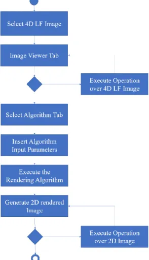
Figure 49. Block diagram of the main steps to execute a certain rendering algorithm. . 40
Figure 50. Snellen chart used before the assessment to test the visual acuity [28]. ... 43
Figure 51. Ishihara plates used before the assessment to test the color blindness [28]. . 43
Figure 52. Developed application used for the quality assessment tests. ... 44
Figure 53. Test material used for the assessment tests. ... 44
Figure 54. Fredo image rendered by SSP and SSPB, PS=11, WS=15. ... 46
Figure 55. Jeff image rendered by SSPB, PS=7, WS=9 and PS=11, WS=15. ... 48
Figure 56. Seagull image rendered by SSPB, PS=9, WS=9 and PS=9, WS=21. ... 49
Figure 57. Zhengyun1 image rendered by DM and DB, α=0.015625, WSP=1.5. ... 50
Figure 58. Laura image rendered by DB, α=0.0625, WSP=1.25 and α=0.0625, WSP=2.00. ... 51
Figure 59. Sergio image rendered by SSPB (PS=11, WS=23) and DB (α=0.0625, WSP=2.00). ... 52
Figure 60. Jeff image rendered by SSP (PS=11) and SSPB (PS=11, WS=15). ... 59
Figure 61. Seagull image rendered by SSP (PS=9) and SSPB (PS=9, WS=13). ... 59
Figure 62. This chart illustrates the winning grouped pairs percentage of this test case. ... 59
Figure 63. Bike image with 3 images with different focal planes: Background (PS=7, WS=9), Middle (PS=9, WS=13), Foreground (PS=11, WS=15). ... 60
Figure 64. Fredo image with 3 images with different focal planes: Background (PS=9, WS=13), Middle (PS=11, WS=15), Foreground (PS=13, WS=19). ... 61
Figure 65. Laura image with 2 images with different focal planes: Background (PS=7, WS=9), Foreground (PS=9, WS=13). ... 61
Figure 66. Jeff image with 3 images with different focal planes: Background (PS=7, WS=9), Middle (PS=9, WS=13), Foreground (PS=11, WS=15). ... 62
Figure 67. Seagull image with 2 images with different focal planes: Background (PS=7, WS=9), Foreground (PS=9, WS=13). ... 63
Figure 68. Sergio image with 3 images with different focal planes: Background (PS=7, WS=9), Middle (PS=9, WS=13), Foreground (PS=11, WS=15). ... 63
Figure 69. Zhengyun1 image with 2 images with different focal planes: Background (PS=7, WS=9), Foreground (PS=9, WS=13). ... 64
Figure 70. Images with 2 focal planes comparison. ... 65
Figure 71. Images with 3 focal planes comparison. ... 65
Figure 72. Images with different blur intensities comparison. ... 69
Figure 73. Sergio image rendered by DM (α=0.0625) and DB (α=0.0625, WSP=1.5). 70 Figure 74. Sergio image rendered by DM (α=0.0) and DB (α=0.0, WSP=1.5). ... 70
Figure 75. Zhengyun1 image rendered by DM (α=0.0625) and DB (α=0.0625, WSP=1.5). ... 71
xv Figure 76. This chart illustrates the winning grouped pairs percentage of this test case. ... 71 Figure 77. Images with different blur intensities comparison. ... 74 Figure 78. This chart illustrates the winning grouped pairs percentage of this test case. ... 75 Figure 79. This chart illustrates half of the Gaussian function to understand the relation between the pixel weight G(x) and half of the window size (x)... 81 Figure 80. This chart illustrates the minimum estimated patch size for different disparity estimation processes, using different values of α. ... 85 Figure 81. This chart illustrates the maximum estimated patch size for different
disparity estimation processes, using different values of α. ... 85 Figure 82. This chart illustrates the average estimated patch size for different disparity estimation processes, using different values of α. ... 85 Figure 83. This chart illustrates the median of the estimated patch size for different disparity estimation processes, using different values of α. ... 86 Figure 84. This chart illustrates the mode of the estimated patch size for different disparity estimation processes, using different values of α. ... 86 Figure 85. This chart illustrates the standard deviation of the estimated patch size for different disparity estimation processes, using different values of α. ... 86
xvii
List of Abbreviations
1D One Dimensional 2D Two Dimensional 3D Three Dimensional 4D Four Dimensional 5D Five Dimensional 7D Seven DimensionalBSI Back Side Illumination CPU Central Processing Unit
DoF Depth of Field
FPS Frames per Second
GPU Graphical Processing Unit GUI Graphical User Interface HDR High Dynamic Range
LF Light Field
MI Micro Image
MLA Micro Lens Array
MP Mega Pixel
PS Patch Size
WS Window Size
WSP Window Size Percentage
BS Block Size
PoV Point of View
AV Angle of view rendering SSP Single-Size Patch rendering
SSPB Single-Size Patch Blending rendering DM Disparity Map rendering
xix
List of Symbols
w Width
h Height
a Disparity Estimation Process Regulation Input Parameter
K Disparity Value
M Number of Individual Pairs N Number of Participants
𝑥𝑖𝑗 Score Given for Image Pair i by Participant j 𝑢̅(𝑖) Average Score of Pair i
𝜎(𝑖) Standard Deviation of Pair i 𝐼𝑆(𝑖) Individual Score of Pair i
𝐼𝑁𝐶(𝑖) Individual Negative Confidence Value of Pair i 𝐼𝑃𝐶(𝑖) Individual Positive Confidence Value of Pair i 𝐼𝐶(𝑖) Individual Confidence Value of Pair i
𝐼𝑊(𝑖) Individual Winner of Pair i 𝐺𝐶
̅̅̅̅(𝑘) Average Group Confidence Value of Group of Pairs k 𝐺𝑆
̅̅̅̅(𝑘) Average Group Score of Group of Pairs k 𝐺𝑊
̅̅̅̅̅(𝑘) Average Group Winner of Group of Pairs k 𝐴𝐶
1
Chapter 1 – Introduction
1.1. Context and Motivation
Recent breakthroughs in light field (LF) technologies for acquiring and manipulating light fields, in areas such as optics and image processing, are creating a revolution in the way of how to acquire, manipulate, share and consume photographic images, a lot further than what is possible today with traditional photographs.
The higher amount of information acquired in 4D light field images, when compared with traditional 2D photographs, allows to change the focal plane, change the viewing perspective of the scene or manipulate the depth of field; functionalities that are not supported by traditional 2D imaging. These breakthroughs are opening new horizons to the human creativity associated to the act of “capture a photo”.
Current display technologies, however, are still not compatible with 4D LF image formats, which means that image rendering algorithms must be used to convert 4D LF content into traditional 2D images, compatible with existing displays.
Consumer-grade 4D LF displays will lead to an authentic breakthrough in terms of visual content consumption and immersive user experiences. However, high quality 2D LF rendering algorithms need to be developed and properly evaluated, which is the main motivation for the work developed in the scope of this dissertation.
In this context, the workplan defined for this dissertation consisted on the development of software tools that allow the user to process and manipulate 4D LF images in an interactive and creative way and on the evaluation of the images produced by these tools, using subjective quality assessment methodologies.
1.2. Objectives
The main goals of this dissertation are, therefore, to study, to implement and to evaluate the rendering process of 2D images from 4D LF content. To reach these goals, two desktop software tools were developed. The first software application, with an easy to use graphical user interface (GUI), allows the user to test different 2D LF rendering algorithms, with the possibility to display and save the rendered images.
The second software application, with a simpler interface, allows to realize quality assessment tests of the rendered 2D images generated in the first software application.
2 Using these two tools, it was possible to determine which of the implemented 2D rendering algorithms can provide better results for diverse types of 4D LF content and rendering scenarios.
1.3. Research Questions
After the work done in this dissertation, valid answers should be provided for the following research questions:
• What type of rendering algorithms will perform better in terms of subjective quality perception?
• What will be the impact of certain algorithm parameters in terms of subjective quality perception?
1.4. Research Method
The research method followed during the development of this dissertation is the Design Science Research Methodology Process Model (DSRMPM), which consists in the following six steps:
• Problem Identification;
• Define Objectives for a solution; • Design and Development; • Demonstration;
• Evaluation; • Communication.
1.5. Structure of the Dissertation
This dissertation is organized into seven chapters that intend to reflect the different work phases until its conclusion.
After the Introduction, Chapter 2 covers the literature review, introducing the most relevant light field concepts, since it is the focus of this dissertation.
3 Chapter 3 reviews and explains different image rendering algorithms that allow the conversion from a 4D light field image into a 2D image. The chapter also suggests an improvement to one of those algorithms that proved to be able to reduce some visual artifacts, increasing the image quality.
Chapter 4 contains a description of the developed rendering application, its implemented algorithms, its architecture and core functionalities.
Chapter 5 describes the subjective quality assessment experiments performed, the used methodology and their setup. The analysis and the conclusions of those quality assessment experiments are presented and discussed in Chapter 6.
Finally, Chapter 7 presents the conclusions of this study and suggests topics for future work.
5
Chapter 2 – Review of Basic Concepts and Technologies
2.1. Basic Concepts
In this chapter, basic concepts such as light field, radiance, focal length, depth of field, 4D light field and light field imaging will be introduced.
2.1.1. Light Field
The idea that a light field should be treated as a field, such as the magnetic field, was first introduced in 1846 by Michael Faraday [1] in a lecture titled “Thoughts on Ray Vibrations”. Faraday defined a 7D function able to capture the evolution of the radiance of all the moving light rays that go through every point in space, in any angular direction, for any wavelength, through time. The function parameterization consisted in a (x, y, z) to specify the 3D spatial position, (θ, φ) to specify the angular direction, one dimension to represent the wavelength and one dimension to represent the time.
In 1991, Adelson [2] was able to simplify the number of the light field function parameters by turning the dimension for the wavelength and time into constants, describing a function able to represent a scene in a single wavelength and instant of time, named plenoptic function, as can be seen in Figure 1.
6 2.1.2. Radiance
Electromagnetic field is carried by elementary particles named photons and the propagation of these particles is called electromagnetic propagation and it is made over electromagnetic waves.
Figure 2 describes the electromagnetic spectrum, where the visible spectrum corresponds to the portion of the electromagnetic field that the human eye can see. The visible spectrum, also known as light rays, correspond to every wavelength from 390 to 700 nm.
Figure 2. Electromagnetic and visible spectrum.
Radiance [3] corresponds to the amount of electromagnetic energy that is emitted, reflected, transmitted or received by a certain surface with a specific angle and direction. Light field cameras use a 2D radiance sensor to be able to capture the amount of light hitting a certain area of the sensor that is measured in (1).
𝐿 = 𝑑
2𝛷
𝑑𝐴𝑑𝛺 cos 𝜃 (1)
In the above equation, L is the radiance of a surface, d is the partial derivative symbol, φ is the radiant flux emitted, reflected, transmitted or received, Ω is the solid angle and A cos θ is the projected area.
7 2.1.3. Focal Length and Angle of View
The focal length [4][5][6], usually represented in millimeters (mm),it is a calculation of an optical distance from the point where light rays converge to form a sharp image of an object to the digital sensor at the focal plane in the camera. Angle of view is the visible extent of the scene captured by the image sensor/film of the camera, which means the bigger the angle of view is, the bigger the area captured is.
Figure 3. Lens with a small focal length and a wide angle of view.
Figure 4. Lens with a big focal length and a small angle of view.
As illustrated by Figure 3 and 4, the angle of view is dependent of the focal length. As the focal length increases, the smaller the angle of view is, and vice versa.
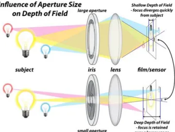
8 2.1.4. Aperture and Depth of Field
Aperture [7][8] is one of the main components in a camera optical system as it defines the size of the opening in the lens that can be adjusted to control the amount of light that reaches the camera sensor. The size of the aperture is measured in millimeters (mm), but aperture is normally described in f-stops and moving from one f-stop to the next doubles or halves the size of the amount of opening in your lens and consecutively the amount of light getting through, as can be seen in Figure 6.
Figure 6. Different apertures and their measures.
Depth of Field [9][10] corresponds to the range of distance that appears acceptably sharp focus in a photograph. Some areas before and after the optimal focal plane are also going to be in focus.
The depth of field outside the sharp focus region will have a gradual blurry transition, even if this fact can be seed by the human eye. Images with small areas of focus are called shallow depth of field, while images with a larger area of focus are called deep depth of field, as can be seen in Figure 7.
The selection of the best depth of field for a certain situation might may vary according to the photographer. The selection of depth of field is therefore a subjective choice.
9 Figure 8. Depth of field of the same light field scene with different apertures. Figure 8 demonstrates the depth of field of two images of the same light field scene with two different apertures. The image on the left has a bigger aperture which result in less depth of field. The image on the right has a smaller aperture which results in a greater depth of field. The higher the aperture is, the bigger the opening in the lens is, the greater the depth of field, and the sharper the background is.
2.1.5. 4D Light Field
As presented before, the plenoptic function has 5 dimensions. It would be extremely hard to capture all the light ray information with current technology, as an extremely large number of sensors and storage devices would be necessary, as explained in [2].
Radiance along a light ray remains constant if there are no objects blocking, as can be seen in Figure 9. Which means the capture of all 5D light rays would have redundant information. That redundant information corresponds to one dimension, reducing the plenoptic 5D parameter function into a 4D function, this discovery was made by Parry Moon and named it photic field in 1981. Computer graphics researchers Levoy and Gortler named it 4D light field in 1996 or Lumigraph respectively, in 1996.
Figure 9. Radiance along a ray remains constant if there are no objects blocking. This way the 4D light field image needs a (x, y) coordinate to specify the 2D spatial position and (θ, φ) coordinate to specify the angular direction.
Traditional 2D video needs a (x, y) coordinate to specify the 2D spatial position and one dimension to represent the time instant.
10 2.1.6. Light Field Image
The Light Field Image also known as plenoptic image, holoscopic image or integral image can be presented as a 2D array of 2D micro images. A possible way to store the 4D information of the light field is presented in Figure 10, in this example all the light field data is stored in the same image. The background image corresponds to a light field image and the image in foreground represents a small highlighted part of the 2D array, where 2D micro images, associated to different perspectives of the light field scene, are placed side by side.
Figure 10. Light Field image / array of micro images example.
Different setups can be used, micro images resolution varies depending on the size of the micro lenses and the content displacement varies depending on the distance from a certain micro lens to their adjacent micro lenses.
This way, micro images resolution is predefined and content displacement from neighboring points of view will depend on the setup used inside the light field camera, used to capture the light field scene.
11
2.2. Light Field Camera Models
This section starts by introducing the basics of the traditional 2D light field cameras followed by a presentation of the basics behind 4D light field cameras. Also, some of the more representative light field cameras, from Lytro and Raytrix manufacturers, will be briefly reviewed.
2.2.1. Basics on Traditional 2D Cameras
As can be observed in the simplified representation depicted in Figure 11, in a traditional camera light rays (represented as arrows) with multiple orientations go through the lens and hit the sensor. The information captured by each pixel of the sensor corresponds to the light intensity from multiple rays hitting the corresponding area of the sensor, originating this way an intensity value of a pixel in the captured image. This process did not change much since the first digital cameras were invented.
Figure 11. Traditional camera simplified optical components representation.
2.2.2. Basics on 4D Light Field Camera – Plenoptic Camera 1.0
Compact Light field cameras are relatively new. Their objective is to capture as much information of the light field scene as possible. To allow this task, a new component, known as micro lens array (MLA), has been added to the camera design, as can be seen in Figure 12. As explained in [11][12], light rays with different intensities and orientations
12 go through the lens, and instead of hitting the sensor like in the traditional cameras, they will go through a certain micro lens, making it possible to store light rays with different orientations, in different parts of the sensor. This process will allow to know the light intensity and the orientation of every single ray. Light field images tend to look like a grid of micro images (MI) and have a lot more information, since they capture the intensity of light in a scene and the direction that the light rays are traveling in space. In this camera, the focal length f is the distance from the sensor to the MLA is fixed. The micro lenses are focused at infinity and completely defocused from the main lens image plane which result in blurry micro images.
Figure 12. Light field camera 1.0 simplified optical components representation.
2.2.3. Basics on 4D Light Field Camera – Plenoptic Camera 2.0
As illustrated in Figure 13 this type of camera is an improvement from the Light Field Camera 1.0, thus includes all its elements. As described in [13] the main (objective) lens creates its image at a plane which is called image plane. In this camera the distance from the sensor to the MLA is fixed at a constant distance of b, the MLA must be at a certain distance a from the image plane in order to obtain a certain fixed focal length f, this relation is described by equation:
1 𝑎+ 1 𝑏= 1 𝑓 (2)
13 With this arrangement, the micro lenses satisfy the lens equation, making them exactly focused on the main lens image plane, resulting in sharp and inverted micro images.
New possibilities like changing the depth of field, changing the point of view and perform depth estimation are now possible to do with a single image, creating a lot of new possibilities to photographers and to the image processing community.
Figure 13. Light field camera 2.0 simplified optical components representation.
2.2.4. First generation Lytro Light Field Camera
Lytro, Inc is an American company founded in 2006 by Executive Chairman Ren Ng, whose PhD research on the field of computational photography / light field imaging won the prize for the best thesis in computer science from Stanford University in 2006. Lytro was the first company releasing a first-generation light field camera into the consumer electronics market, in 2012. More information about this light field 1.0 camera with 11 megaray sensor camera can be found in [14].
14 2.2.5. Second generation Lytro Light Field Camera – Lytro Illum
In 2014 their second-generation camera named Lytro Illum was also a light field 1.0 camera and was released with a 40 megaray sensor, with a lot more powerful processor and with a display overlay that shows the photographer the relative focus of all objects in the frame, and which elements are re-focusable.
Figure 15. Second generation Lytro Light Field Camera – Lytro Illum [14].
Lytro is expanding into cinematography, virtual reality and augmented reality areas and released a new camera called Lytro Immerge whose main innovation is the way of recording light field information [14].
2.2.6. Raytrix R42 Light Field Camera
Raytrix GmbH [15], in a German company founded in 2009. Since 2010 they are selling 3D cameras for industrial applications and research purposes. With a team of 15 people, their main goal is to improve the quality of their light field cameras and to explore new application areas.
At least seven different light field cameras are presented in Raytrix website [15], some of them are aimed for video, other for still imaging.
15
2.3. Light Field Camera Arrays
A different way to capture the light field is using different arrangements of camera arrays [16], as illustrated in Figure 17. The reduced cost of cameras makes it possible to replace the monocular camera with an array of cameras in certain situations, as presented in [17]. Different arrangements will change the dynamic range, the resolution, seeing through occlusions and in the depth estimation of the scene.
Figure 17. Light field camera array [17].
2.4. Light Field Standardization Initiatives
Light Field imaging has currently risen as a feasible and prospective technology for future image and video applications. New standardizations for light field imaging are emerging [18][19].
2.4.1. MPEG-I
MPEG-I is the name of the new work that was started by the Moving Picture Experts Group (MPEG) which targets future immersive applications. The goal of this new standard is to enable various forms of audio-visual immersion, including panoramic video with 2D and 3D audio, with various degrees of true 3D visual perception.
2.4.2. JPEG Pleno
JPEG Pleno standardization was launched by the Joint Photographic Experts Group (JPEG) and aims to provide a standard framework for representing new imaging modalities, like texture-plus-depth, light field, point cloud and holographic imaging.
17
Chapter 3 – Light Field Rendering
This chapter introduces the developed lenslet rendering solutions, for plenoptic 2.0 cameras, that were based in some references from the state of the art and allow to render 4D LF content into 2D displays. All the algorithms were implemented from scratch, some of the difficulties and decisions made in the development process will be explained. Other implemented ideas to improve the algorithms quality will also be described.
3.1. Rendering Solutions Input
This section introduces the schematic representations of a light field image and of a micro image that will be used in further sections, where different rendering solutions that allow to render 4D light field contents into 2D displays will be presented.
Light Field technology allows a user to take a 4D photo, convert to 2D using a rendering algorithm such as the ones proposed in [19]-[23], change the light field perspective of the scene, estimate the depth of the scene and manipulate the depth of field.
Figure 18. Light field image, with 6 micro images, schematic representation
Figure 18 is a schematic representation of a 4D light field image that can also be a 2D array of micro images, where each micro image is associated to a certain position (i, j). Each micro image is the result of several different light rays that went through a certain micro lens and captured by the radiance sensor. The valid values for i and j are:
0 ≤ 𝑖 < 𝑀𝐿𝐴. ℎ𝑒𝑖𝑔ℎ𝑡
0 ≤ 𝑗 < 𝑀𝐿𝐴. 𝑤𝑖𝑑𝑡ℎ (3) where MLA.height and MLA.width represent the vertical and horizontal dimensions of the micro lens array, respectively.
Figure 19. Micro image, with 9 pixels, schematic representation.
As can be seen in Figure 19, inside each micro image (MI) there are several pixels, where each pixel is associated to a certain position (row, col), the valid row and col values are described in (4).
0 ≤ 𝑟𝑜𝑤 < 𝑀𝐼. ℎ𝑒𝑖𝑔ℎ𝑡
18
3.2. Texture Based 2D Image Rendering Solutions
3.2.1. Angle of View Based 2D Image Rendering (AV)
The idea behind this algorithm [19] starts by choosing the scene perspective to be seen, in other words, a valid position (row, col) inside a micro image, must be chosen. To create the new image, which will have the same size as the micro lens array (MLA), the intensity value of the pixel in the selected position (row, col) will be extracted from each micro image (i, j) and stored in the corresponding position (i, j) of the new image. This way, a certain perspective (row, col) of the light field scene will be rendered.
Assuming Figure 18 is the light field image this algorithm is using as input, it will be able to render the 9 different and possible perspectives represented in Figure 20, as this is the number of pixels inside each MI, with the size of the MLA, in this case, 2 rows and 3 columns.
Figure 20. The 9 different rendered perspectives.
Advantages: Since only one pixel is extracted from each MI to render one of the perspectives, this algorithm has the high number of perspectives that can be rendered.
Disadvantages: Since only one pixel is extracted from each MI to render one of the perspectives, the resolution of the rendered images will be always equal to the size of the
19 MLA, and typically these values are very small compared to images seen daily all over the internet.
Figure 21. Rendering with the AV algorithm, with the developed software tool.
As can be seen by Figure 21, a generated perspective from the light field scene from this rendering algorithm have been up scaled in size by a factor of five due to the small resolution of these output images. The images have a bad quality and are very pixelated, being hard to understand the details of their content.
3.2.2. Single-Size Patch Based 2D Image Rendering (SSP)
This algorithm was developed by Todor Georgiev [20], in 2010, and is very similar to the one presented in the previous section but instead of extracting a single pixel from each MI, will extract a squared block of pixels with a fixed size, referred as patch size (PS), which can assume the values:
1 < 𝑃𝑆 < min(𝑀𝐼. ℎ𝑒𝑖𝑔ℎ𝑡, 𝑀𝐼. 𝑤𝑖𝑑𝑡ℎ) (5)
A position (row, col) must be selected and will correspond to the top left pixel of the block that will be extracted. The valid values for the row and col vary depending of the selected patch size, as defined in:
20 0 ≤ 𝑟𝑜𝑤 < 𝑀𝐼. ℎ𝑒𝑖𝑔ℎ𝑡 − 𝑃𝑆
0 ≤ 𝑐𝑜𝑙 < 𝑀𝐼. 𝑤𝑖𝑑𝑡ℎ − 𝑃𝑆 (6)
The patch size parameter which corresponds to the number of pixels extracted from each MI, which means the bigger the patch size is, the bigger the resolution will be, making the resolution of the resulting image proportional to the value of the patch size as described by the following equation:
𝑃𝑒𝑟𝑠𝑝𝑒𝑐𝑡𝑖𝑣𝑒. ℎ𝑒𝑖𝑔ℎ𝑡 = 𝑀𝐿𝐴. ℎ𝑒𝑖𝑔ℎ𝑡 × 𝑃𝑆
𝑃𝑒𝑟𝑠𝑝𝑒𝑐𝑡𝑖𝑣𝑒. 𝑤𝑖𝑑𝑡ℎ = 𝑀𝐿𝐴. 𝑤𝑖𝑑𝑡ℎ × 𝑃𝑆 (7)
The number of different perspectives will also be dependent of the same parameter, as the bigger the patch size is, the smaller the number of different perspectives that can be rendered will be as shown in equation:
#𝑃𝑒𝑟𝑠𝑝𝑒𝑐𝑡𝑖𝑣𝑒𝑠 = [𝑀𝐼𝐻𝑒𝑖𝑔ℎ𝑡− (𝑃𝑎𝑡ℎ𝑆𝑖𝑧𝑒− 1)] × [𝑀𝐼_𝑊𝑖𝑑𝑡ℎ − (𝑃𝑎𝑡ℎ_𝑆𝑖𝑧𝑒 − 1)] (8)
Assuming Figure 18 is the light field image this algorithm is using as input and the patch size is equal to 2, it will be able to render 4 different perspectives as defined in (8) and represented in Figure 22, with the double of the MLA size, as defined in (7).
Figure 22. The 4 different rendered perspectives with a patch size of 2.
Advantages: The rendered images will no longer have small resolutions as the ones obtained with the AVe algorithm, because this algorithm extracts more than one pixel per MI.
21 Disadvantages: The bigger the patch size is, a bigger number of pixels will be extracted from each MI, which will reduce the number of different rendered perspectives.
Figure 23. Rendering with the SSP algorithm, with the developed software tool.
The rendering in Figure 23 has a lot better quality when compared to the rendering from the AVe algorithm. The transitions between neighbor squared blocks are clear, especially in the background. Looking to the girl arm there was a problem with one of the micro lenses.
3.2.3. Single-Size Patch Blending Based 2D Image Rendering (SSPB)
This algorithm is identic to the one presented in the previous section, was developed by Todor Georgiev and Andrew Lumsdaine and is described in [21][22]. The patch size parameter already introduced, will represent, once again, the size of the block of pixels that will be extracted from each MI. A selected valid position (row, col) will mark the starting point where the block will be extracted. Instead of joining side by side the extracted blocks in the new image, a process called blending will be used, where the main goal is to smooth the transitions by calculating the average between pixels, with different weights, from neighbor blocks.
To be able to make this blending process a few more parameters will be needed. A new parameter like the patch size will be needed, which will be named window size (WS). In this algorithm the patch size and window size will be assumed as both being odd numbers and the following conditions must be valid:
22 1 < 𝑃𝑆 ≤ 𝑊𝑆 < min(𝑀𝐼. ℎ𝑒𝑖𝑔ℎ𝑡, 𝑀𝐼. 𝑤𝑖𝑑𝑡ℎ) (9)
In Figure 24 a representation of a block extracted from a MI is presented with a patch size of 3 and a window size of 5.
Figure 24. Extracted block from a MI.
The first step is to associate each pixel of the extracted block with a certain weight, this means the further away a pixel is from the center of the block, the smallest the weight of that pixel will have. To make this possible, the weight of each pixel is given by:
𝑊𝑒𝑖𝑔ℎ𝑡(𝑟𝑜𝑤, 𝑐𝑜𝑙) = 1 × 𝑒− (𝑟𝑜𝑤−𝑐𝑒𝑛𝑡𝑒𝑟𝑅𝑜𝑤)2 2×𝑠𝑖𝑔𝑚𝑎𝑌2 × 𝑒 −(𝑐𝑜𝑙−𝑐𝑒𝑛𝑡𝑒𝑟𝐶𝑜𝑙) 2 2×𝑠𝑖𝑔𝑚𝑎𝑋2 (10)
In equation (10), weight corresponds to the weight of a certain pixel, given by the influence of horizontal and vertical gaussian function, (row, col) correspond to the position of a certain pixel, (centerRow, centerCol) correspond to the position of the pixel in the center of the block (centered in the middle of the extracted block of size WS), in this case position (centerRow = 2, centerCol = 2) and (sigmaY, sigmaX) have a big influence in the format of the horizontal and vertical gaussian functions, used in equation (10), as can be seen in Figure 25. For more information about the relation between the WS and the components of the sigma parameter consult Appendix A.
Figure 25. Graph with the influence of the sigma parameter in a Gaussian function.
-0.5 0 0.5 1 1.5 -20 -10 0 10 20 W eight
Distance to Center Position
Influence of Sigma in Gaussian
Function
Sigma = 0.5 Sigma = 0.75 Sigma =1 Sigma = 2 Sigma = 523 Figure 25 shows the influence of the parameter sigma in the format of the Gaussian function as the smaller the sigma is, the fastest the weight of the pixels closest to the center will decrease.
Figure 26. Light field image with only 2 micro images.
Assuming the light field images used by this algorithm was the one presented in Figure 26, with a patch size of 3 and a window size of 5, a resulting image is returned with the size of the chosen patch size times the number of micro images, which means an image with 3 rows and 6 columns.
As the output image will have the size of multiple patch sizes, some of the pixels inside the window size, presented as the white pixels in the margins, will overlap with pixels of the neighbor micro image, as presented in Figure 27.
Figure 27. Resulting image with overlapping pixels from neighbor blocks and invalid pixels.
As the white pixels after the margin will be removed as they won’t have a pixel position inside the output image, as can be seen in Figure 28.
Figure 28. Resulting image with overlapping pixels from neighbor blocks.
As shown in Figure 28 there are some pixels that have contributions of n=2 sub pixels from the input image (the n can vary depending on the relation between PS and WS), in these situations the following equation should be applied:
24 𝑝𝑖𝑥𝑒𝑙𝐶𝑜𝑙𝑜𝑟 = ∑ (𝑐𝑜𝑙𝑜𝑟𝑖× 𝑤𝑒𝑖𝑔ℎ𝑡𝑖) 𝑛 𝑖=0 ∑𝑛𝑖=0𝑤𝑒𝑖𝑔ℎ𝑡𝑖 (11)
To calculate the average of all the neighbor contributions with different weights as can be seen in Figure 29 and place the result as the final pixel color, resulting in an output image illustrated in Figure 30.
Figure 29. Determine final pixel color using (11), with a weight of 0.6 for color pixels and 0.4 for white pixels.
Figure 30. Algorithm output image with smooth transitions between blocks.
Advantages: The smooth transitions between blocks makes harder for the user to see artifacts when compared to the SSP algorithm where the outline of each block could be easily seen.
Disadvantages: Comparing this algorithm with AV and SSP, this is the algorithm with less perspectives due the fact that is the one taking more information (patch size and window size) from the input image to render a perspective of the light field scene. This is also the less efficient algorithm as is the most complex one so far.
25 The rendering in Figure 31 is the one with better quality between the three algorithms presented. The transitions between neighbor squared blocks are less clear, except in the background. Looking to the girl arm there was a problem with one of the micro lenses, but with the blending process the reason is no longer clear if that is a problem or if it is a spot on her skin.
3.3. Disparity Based 2D Image Rendering Solutions
In this section, two models of how to estimate the disparity map are presented and then two algorithms that use the disparity map estimated to get an all-in-focus rendered 2D image are introduced.
3.3.1. Disparity Estimation
This disparity estimation model is explained by T. Georgiev and A. Lumsdaine in [20].
Figure 32. Light field image with 9 micro images of size 7 by 7.
If our 4D light field image is the one presented in the Figure 32, the first thing to do is to specify the row, col and the block size (BS) of pixels to compare with all the blocks of the adjacent micro images in order to find out the block with the most similarities, and that corresponds to the displacement value between the two micro images.
26 Figure 33. Estimation of the disparity of micro image 1, 1 with their neighbors.
Assuming the point of view corresponds to row = 2, col = 2 and the block size = 3, as presented in Figure 33, where for each micro image, a comparison between the red block of the micro image of which its disparity is tried to be estimated and all the blocks in the same vertical line for the top and bottom micro images and with all the blocks in the same horizontal line for the left and right micro images, represented by blue lines in Figure 33.
Figure 34. Estimation of the disparity of micro image 1, 1 with its right neighbor.
Figure 34 shows how the disparity value is calculated, representing all the possible comparisons that must be done in this case. For each comparison of blocks the following equation must be performed:
𝑐𝑜𝑚𝑝𝑎𝑟𝑖𝑠𝑜𝑛 =
∑𝑟𝑜𝑤𝑠𝑟=𝑜 ∑𝑐𝑜𝑙𝑠𝑐=0(𝐴𝑟𝑐−𝐵𝑟𝑐)2 𝑟×𝑐
27 The equation will calculate the square differences of the blocks A and B, calculate the square difference value per pixel and divide it by 255 to get a value between one and two hundred and fifty-five, this way, the equation will return two hundred and fifty-five if the two blocks are completely different and zero if the two blocks are equal.
In this case, when a comparison of the red square is made with the five possible blocks from the right micro image, a calculation of the column value of the block that obtained the highest comparison value with the red block is needed. After comparing the red block with all the possible blocks, the equation:
𝐾𝑥= |𝑐𝑜𝑙 − 𝑐𝑜𝑙max_𝑐𝑜𝑚𝑝𝑎𝑟𝑖𝑡𝑖𝑜𝑛| (13)
should be used to calculate the horizontal disparity value between the two micro images. To calculate the vertical disparity value between the two micro images, the following equation should be used:
𝐾𝑦= |𝑟𝑜𝑤 − 𝑟𝑜𝑤max_𝑐𝑜𝑚𝑝𝑎𝑟𝑖𝑡𝑖𝑜𝑛| (14)
For this case, after performing all the comparisons, the column = 3 would have the lowest comparison value, so Kx = |2-3|=1.
After performing the same logic to all the valid neighbors, the following equation should be used:
𝐾 =𝐾𝑥𝑙𝑒𝑓𝑡+ 𝐾𝑥𝑟𝑖𝑔ℎ𝑡+ 𝐾𝑦𝑡𝑜𝑝+ 𝐾𝑦𝑏𝑜𝑡𝑡𝑜𝑚
# 𝑜𝑓 𝑣𝑎𝑙𝑖𝑑 𝑛𝑒𝑖𝑔ℎ𝑏𝑜𝑟𝑠 (15)
to calculate the average disparity value for each one of the nine micro images, as illustrated in Figure 35. 𝐾00= 𝐾𝑥𝑟𝑖𝑔ℎ𝑡+ 𝐾𝑦𝑏𝑜𝑡𝑡𝑜𝑚 2 = |2 − 3| + |2 − 3| 2 = 2 2= 1 𝐾01= 𝐾𝑥𝑙𝑒𝑓𝑡+ 𝐾𝑥𝑟𝑖𝑔ℎ𝑡+ 𝐾𝑦𝑏𝑜𝑡𝑡𝑜𝑚 3 = |2 − 1| + |2 − 3| + |2 − 3| 3 = 3 3= 1 𝐾02= 𝐾𝑥𝑙𝑒𝑓𝑡+ 𝐾𝑦𝑏𝑜𝑡𝑡𝑜𝑚 2 = |2 − 1| + |2 − 3| 2 = 1 + 1 2 = 1 𝐾10 = 𝐾𝑥𝑟𝑖𝑔ℎ𝑡+ 𝐾𝑦𝑡𝑜𝑝+ 𝐾𝑦𝑏𝑜𝑡𝑡𝑜𝑚 3 = |2 − 3| + |2 − 1| + |2 − 3| 3 = 3 3= 1 𝐾11 = 𝐾𝑥𝑙𝑒𝑓𝑡+ 𝐾𝑥𝑟𝑖𝑔ℎ𝑡+ 𝐾𝑦𝑡𝑜𝑝+ 𝐾𝑦𝑏𝑜𝑡𝑡𝑜𝑚 4 = |2 − 1| + |2 − 3| + |2 − 1| + |2 − 3| 4 = 4 4= 1
28 𝐾12 = 𝐾𝑥𝑙𝑒𝑓𝑡+ 𝐾𝑦𝑡𝑜𝑝+ 𝐾𝑦𝑏𝑜𝑡𝑡𝑜𝑚 3 = |2 − 1| + |2 − 1| + |2 − 3| 3 = 3 3= 1 𝐾20= 𝐾𝑥𝑟𝑖𝑔ℎ𝑡+ 𝐾𝑦𝑡𝑜𝑝 2 = |2 − 3| + |2 − 1| 2 = 2 2= 1 𝐾21= 𝐾𝑥𝑙𝑒𝑓𝑡+ 𝐾𝑥𝑟𝑖𝑔ℎ𝑡+ 𝐾𝑦𝑡𝑜𝑝 3 = |2 − 1| + |2 − 3| + |2 − 1| 3 = 3 3= 1 𝐾22= 𝐾𝑥𝑙𝑒𝑓𝑡+ 𝐾𝑦𝑡𝑜𝑝 2 = |2 − 1| + |2 − 1| 2 = 2 2= 1
Figure 35. Disparity Map after the estimation of the disparity for each micro image and the calculations performed to obtain those values.
After performing the disparity estimation for all the existing micro images by placing the red block in the point of view row = 2, col = 2 and comparing it with all the neighbors, a disparity value would show for each micro image, that would look like the disparity map in Figure 35.
29 Figure 36 illustrates the estimated disparity map for the image that was used to display the results from the previous introduced algorithms.
The original values of the disparity map were multiplied by a factor of ten to obtain bigger visual differences between the disparity values. The darker pixels correspond to small disparity values, that means they don’t change much their position from micro image to micro image and they are in the background of the image. The lighter pixels correspond to bigger disparity values that often change their position from micro image to micro image and they are in the foreground.
3.3.2. Disparity Estimation – Minimizing Errors with α
Small errors in the estimation of disparity create artifacts that can have a big visual impact for the user, this happens because when the estimated PS is wrong, the extracted blocks will not match after being upscaled and placed side by side.
So, a new adaptive estimation model that allows the user to have some control of the estimation process is presented by introducing a new parameter called alpha (α). The difference from the disparity estimation model presented in Section 3.2.1. to this one is to have a dependent factor of the final estimated PS values of the left and top adjacent micro images. To introduce this new factor, equation 12 must be replaced for a more robust equation, as presented:
𝑐𝑜𝑚𝑝𝑎𝑟𝑖𝑠𝑜𝑛 = ∑𝑟𝑜𝑤𝑠𝑟=𝑜 ∑𝑐𝑜𝑙𝑠𝑐=0(𝐴𝑟𝑐−𝐵𝑟𝑐)2 𝑟×𝑐 255 + |𝑐𝑢𝑟𝑟𝑒𝑛𝑡𝐷𝑖𝑠𝑝.−𝑎𝑣𝑔𝑁𝑒𝑖𝑔ℎ𝑏𝑜𝑟𝐷𝑖𝑠𝑝.| 𝑚𝑎𝑥𝑃𝑜𝑠𝑠𝑖𝑏𝑙𝑒𝐷𝑖𝑠𝑝. × 𝛼 (16)
the currentDisp. corresponds to the disparity value of the center of the block that is being compared with the red block and is calculated using:
𝑐𝑢𝑟𝑟𝑒𝑛𝑡𝐷𝑖𝑠𝑝. = {|𝑐𝑜𝑙 − 𝑐𝑜𝑙𝑐𝑢𝑟𝑟𝑒𝑛𝑡_𝑐𝑜𝑚𝑝𝑎𝑟𝑖𝑡𝑖𝑜𝑛| , ℎ𝑜𝑟𝑖𝑧𝑜𝑛𝑡𝑎𝑙 𝑛𝑒𝑖𝑔ℎ𝑡𝑏𝑜𝑟 |𝑟𝑜𝑤 − 𝑟𝑜𝑤𝑐𝑢𝑟𝑟𝑒𝑛𝑡_𝑐𝑜𝑚𝑝𝑎𝑟𝑖𝑡𝑖𝑜𝑛| , 𝑣𝑒𝑟𝑡𝑖𝑐𝑎𝑙 𝑛𝑒𝑖𝑔ℎ𝑏𝑜𝑟
(17)
The avgNeightborDisp. corresponds to the average of two neighbors for which their final disparity value has already been estimated. In this case, the neighbors from the micro images on the top and on the left are used. The value of the average neighbor disparity is given by equation:
𝑎𝑣𝑔𝑁𝑒𝑖𝑔ℎ𝑏𝑜𝑟𝐷𝑖𝑠𝑝. =𝐾𝑙𝑒𝑓𝑡_𝑛𝑒𝑖𝑔ℎ𝑡𝑏𝑜𝑢𝑟+ 𝐾𝑡𝑜𝑝_𝑛𝑒𝑖𝑔ℎ𝑡𝑏𝑜𝑢𝑟
30 The maxPossibleDisp. Corresponds to the maximum disparity value that a certain micro image can have and its given by:
𝑚𝑎𝑥𝑃𝑜𝑠𝑠𝑖𝑏𝑙𝑒𝐷𝑖𝑠𝑝. = min(𝑟𝑜𝑤, 𝑐𝑜𝑙, 𝑀𝐼. ℎ𝑒𝑖𝑔ℎ𝑡 − 1 − 𝑟𝑜𝑤, 𝑀𝐼. 𝑤𝑖𝑑𝑡ℎ − 1 − 𝑐𝑜𝑙) (19)
As can be seen by the equation 16, the equation has contributions of the final estimated PS values calculated for the micro images on the left and on the top, minimizing possible errors in the estimation of the PS value for the current micro image.
Next, from Figures 38-43 the disparity maps for the following sequence of images (Figure 37) are presented, varying the parameter α.
Figure 37. Image Sequence used to estimate the disparity maps with different α values.
Figure 38. Disparity Maps with α = {0.0, 0.015625, 0.0625, 0.25} for the image Laura.
31 Figure 40. Disparity Maps with α = {0.0, 0.015625, 0.0625, 0.25} for the image Jeff.
Figure 41. Disparity Maps with α = {0.0, 0.015625, 0.0625, 0.25} for the image Seagull.
Figure 42. Disparity Maps with α = {0.0, 0.015625, 0.0625, 0.25} for the image Sergio.
Figure 43. Disparity Maps with α = {0.0, 0.015625, 0.0625, 0.25} for the image Zhengyun1.
After analyzing all the rendered images for each image of the sequence with the following a values {0.0, 0.0078125, 0.015625, 0.03125, 0.0625, 0.125, 0.25, 0.50} was concluded that the rendered images with values around α = 0.015625 and α = 0.0625 have less artifacts than the ones with α = 0 (α = 0 corresponds to equation 12 which means the estimation model used is the one introduced in Section 3.2.1.), for more information consult Appendix B.
32 3.3.3. Disparity Map Based 2D Image Rendering (DM)
This 2D rendering algorithm was developed by Todor Georgiev and Andrew Lumsdaine [20] and can be seen as an optimization of the SSP algorithm introduced in Section 3.1.2., but instead of having a fixed patch size, it has multiple patch sizes to try to focus all the different planes of the image. The estimation of the disparity will be needed, to determine the patch size that better matches its neighbor patches. As the goal is to have an all-in-focus image, each different patch size value will allow to focus a certain focal plane, where identical patch sizes correspond to objects at a certain depth in the scene. Since the patches extracted from the different micro images have different sizes, un upscaling process will be needed to guaranty that all the extracted blocks have the same size before placing them side by side in the resulting image.
This way, an estimation of the disparity map (introduced in Section 3.4.1 or 3.4.2) is done for the light field image. Since a row and col were selected to define the position of the block used to calculate the disparity map, each micro image should get its estimated PS value and recalculate the right row and col to guaranty that all the patch sizes are centered in the same pixel, which means that a calculation to obtain the newRow should be performed using equation:
𝑛𝑒𝑤𝑅𝑜𝑤 = 𝑟𝑜𝑤 +𝑏𝑙𝑜𝑐𝑘_𝑠𝑖𝑧𝑒
2 −
𝑝𝑎𝑡𝑐ℎ𝑠𝑖𝑧𝑒
2 (20)
and the same should be done to obtain newCol using equation:
𝑛𝑒𝑤𝐶𝑜𝑙 = 𝑐𝑜𝑙 +𝑏𝑙𝑜𝑐𝑘_𝑠𝑖𝑧𝑒
2 −
𝑝𝑎𝑡𝑐ℎ𝑠𝑖𝑧𝑒
2 (21)
After getting the different patch sizes extracted from the different micro images, all the extracted pixel blocks must have the same size, so an upscaling to the maximum disparity value in the disparity map is necessary.
When all the extracted images have the same size, the arrangement is done side by side, as shown in the SSP algorithm in Section 3.3.2. and then the final rendered image is obtained.
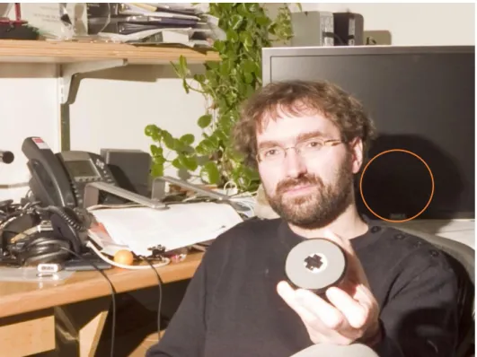
Figure 44 and 45 show two results of the same light field image, the first one uses the first disparity estimation model introduced in Section 3.2.1. (α = 0) and the second image uses the second disparity estimation model with an α = 0.0625. If the artifact area inside the orange circle is analyzed, the second image has better results than the first one.
33 Figure 44. Fredo image using the DM algorithm with α = 0.0.
Figure 45. Fredo image using the DM algorithm with α = 0.0625.
Advantages: This is the first rendering algorithm that can display an all-in-focus 2D image.
Disadvantages: Since an upscaling process must be done to make sure all the extracted blocks have the same size, errors can be introduced in this process, depending on how much a certain block must be upscaled. Other visible disadvantage is the fact that this algorithm does not have any blending process associated so the outline of the different blocks can be seen in some areas of the image.
34 3.3.4. Disparity Blending Based 2D Image Rendering (DB)
The idea behind this algorithm is similar as the one explained by João Lino in [17] and is like the one presented in Section 3.2.3. except it has the blending process that has been introduced in the SSPB algorithm in Section 3.1.3. Since the disparity estimation models introduced in Section 3.2.1 and 3.2.2. are used again, different micro images might be associated with a different patch sizes, so, specifying a single window size won’t work. For that reason, a new input parameter must be introduced. This way, Window Size Percentage (WSP) corresponds to a percentage that will be multiplied for each patch size to find out what is the right window size for each micro image.
Once the window size is known for each micro image, a block of pixels with that size must be extracted from each micro image and again different blocks are presented with different sizes, so the upscaling process is necessary to make sure that all the blocks have the size of the biggest patch size, found in the disparity map, multiplied by the Window Size Percentage parameter. Just like in the SSPB algorithm all the patch sizes and window sizes in this algorithm should be odd numbers.
After executing the upscale process, the application of the blending process is necessary at the exact same way it was applied in the SSPB algorithm.
Figure 46 shows the Fredo image where a considerably better result of the artifact area inside the orange circle is seen.
35
Chapter 4 – Developed Rendering Application
4.1. Technologies
On the planning stage of the development process of this desktop application, a decision was made to select the programming language and libraries that were going to be used. The main goal was to create open source and independent tools that would easily work in different platforms with an easy to use graphical user interface.
Java was the selected programming language due to some of its characteristics such as:
• Automatic memory allocation; • Garbage collection;
• Object oriented, allowing the creation of modular programs and reusable code; • Platform-independent making it easy to run the application in different systems; • Multithreading, having the capability for a program to perform several tasks
simultaneously.
Swing is part of the Oracle’s Java Foundation Classes (JFC) which is an API for providing a graphical user interface for Java programs. Since it is part of the Java Standard Edition Development Kit [23], the tools needed were already being used to be able to create a custom and easy to use graphical user interface, who would work regardless of whether the underlying user interface system is Windows, macOS or Linux.
OpenCV (Open Source Computer Vision Library) [24] is completely free for academic use, it has C++, Python and Java interfaces and supports Windows, Linux, macOS, iOS and Android. This library was designed for computational efficiency and a strong focus on real-time applications. The big community behind it and the quality of their documentation was also a big part of why this library was chosen.
Eclipse [25] was the chosen IDE due to its big affiliation to the open source and Java communities. Setting up the development environment on eclipse IDE with Java SE Development Kit1.7 and OpenCV 3.4.0 was simpler and faster when compared to some other environments such as C++ and OpenCV on Visual Studio IDE.
36
4.2. Graphical User Interface
The main software application is completely free and easy to use, where the user can try all the implemented algorithms, manipulate the algorithm parameters (see Figure 47), check the result in the full screen mode and save the perfect 2D image, by selecting the best focal plane and the best point of view of the light field scene.
Figure 47. Print screen of the main desktop application.
This software might be useful for the image processing community as a content generator for objective and subjective tests. It is open source to allow contributions from other authors to make the application as robust as possible.