oligopoly
José Pedro Pontes
This paper examines the location of three vertically-linked firms. In a spatial economy composed of two regions, a monopolist firm supplies an input to two consumer goods firms that compete in quantities. The interaction between the firms is modelled by means of a three-stage game, where the firms first select locations, then the upstream firm chooses thedelivered prices of the intermediate good, and finally the downstreamfirms select quantities of the final good. It is concluded that agglomeration is more likely to occur when the ratio between the transport cost of the intermediate good and the transport cost of the final good is higher. If this proportion is low, the existence of an agglomeration varies nonmonotonically with transport costs.
Keywords: Agglomeration, Intermediate Goods, Spatial Oligopoly.
J.E.L. Classification: R30, L13,C72.
Author’s affiliation: Instituto Superior de Economia e Gestão, Technical University of Lisbon and Research Unit on Complexity in Economics (UECE).
Mailing Address: Instituto Superior de Economia e Gestão, Rua Miguel Lupi, 20, 1249-078 Lisboa Portugal.
Tel. +351 21 3925916
Fax +352 21 3922808
Email <[email protected]>
1
Introduction
In the absence of labor mobility, the agglomeration of productive activity follows from interactions between firms. As noted by MARSHALL (1920), these interactions can be technological, e.g. spillovers which are not mediated by the market, or they can take the form of an exchange of intermediate goods. In this case, the saving in the transport cost of intermediate goods is a powerful incentive for the agglomeration of vertically-related firms.
In the literature that addresses this issue, the locational interaction of vertically-related firms is modeled in the following way. An imperfectly competitive upstream industry supplies an intermediate good to a down-stream industry, which can be either perfectly or imperfectly competitive. While AMITI (2001), FUJITA and HAMAGUCHI (2002) and FUJITA and THISSE (2002) assume that the downstream industry is perfectly competi-tive, VENABLES (1996) and BELLEFLAMME and TOULEMONDE (2003) make the opposite assumption that thefinal industry is imperfectly compet-itive. It is further assumed that the intermediate good and the consumer good have different transport costs, which vary independently.
(2003), the cost linkage follows from the increased competition brought about by the agglomeration in the upstream industry that decreases the price of the intermediate good and the production costs of consumer goods firms. The strength of the cost linkage effect is proportional to the transport cost of the intermediate good.
With this framework, the literature concludes that agglomeration occurs when the transport cost of the intermediate good is high in relation to the transport cost of the final good. In this case, no downstream firm has any incentive to choose an isolated location, as this move would not greatly de-crease the delivery cost of thefinal good and would substantially increase the transport cost of the required input. Furthermore no input supplier would gain by leaving the agglomeration, as it would have to bear the high transport cost of the intermediate good to thefinal goodsfirms (FUJITA and THISSE, 2002). If the transport cost of the intermediate good is lowered in relation to the transport cost of the consumer good, a dispersion of downstream firms can occur (FUJITA and HAMAGUCHI, 2002).
A common assumption in this literature is that the transport costs of the intermediate good and the final good vary independently. In fact, the transport costs of the intermediate good and of the final good vary in pro-portion as they are both influenced by the general quality of the transport and communication infrastructure. Hence, KRUGMAN and VENABLES (1995) assume a Dixit-Stiglitz monopolistically competitive industry where each variety is both a consumer good and an intermediate good used by each
firm. Under this assumption, they conclude that thefirms disperse for high transport costs in order to relax competition and serve the local demand. For low transport costs, the competition effect is no longer important, and thefirms agglomerate in order to make full use of cost linkages. 1
The major inconvenience with this result is that it implies that the degree of divisibility of the upstream and downstream industries is the same. The classical paper by KOOPMANS and BECKMANN (1957) shows that the issue of the location of firms that engage in input transactions is non trivial if the degree of divisibility of the vertically-related industries is different. Otherwise, the transport costs of the intermediate good can be avoided by jointly locating a fraction of the upstream and a fraction of the downstream
1For very low transport costs, if wages are elastic to employment, thefirms can disperse
industries. With this assumption, BELLEFLAMME and TOULEMONDE (2003) conclude that a symmetric division of upstream and downstreamfirms between the regions is always an equilibrium.
In this paper, it is assumed that the number of firms in the two indus-tries is different. A monopolist firm supplies an intermediate good to two downstreamfirms that compete in quantities in the market of thefinal good. Implicitly, economies of scale are supposed to be more important in the upstream than in the downstream industry. Firstly, the firms decide their locations in two regions. Then, the upstream firm selects the delivered price of the input and finally the downstream firms compete in quantities. The transport costs of the intermediate good and of the consumer good vary in proportion. Although the set of equilibria of this game is not characterized, an attempt is made to assess whether or not there exists a full agglomeration equilibrium for different values of the transport costs.
Basically, the increase in transport costs has two opposing effects on the existence of agglomeration. On one hand, an increase in the transport cost of the intermediate good helps to develop agglomeration because it strengthens the advantage of the input supplier’s location as a low production cost site for each final producer. The higher the transport cost of the intermediate good in relation to the transport cost of the final good, the stronger is this effect.
On the other hand, an increase in the transport cost of the consumer good encourages the downstreamfirms to become geographically isolated in order to relax intra-regional competition and to be close to local consumers. The fact that the increase in the transport costs has two opposite effects upon the location of the consumer goodsfirms makes it likely that the relationship between the general level of transport costs and the agglomeration of firms will be nonmonotonic.
generalizes the ”U inverted” pattern that was obtained by KRUGMAN and VENABLES (1995) and VENABLES (1996) in the sense that agglomeration and dispersion alternate when the transport costs vary.
In section 2, a three-stage noncooperative game is presented. The main conclusions are drawn in section 3.
2
The model
2.1
Assumptions
We suppose a spatial economy that obeys the following assumptions:
1. The economy has two regions A andB with the same number of con-sumers. Units are chosen so that this number is normalized to 1. The distance between the regions is1by convention. The distance between two points in the same region is zero.
2. There are two vertically-related industries. A downstream industry produces a homogeneous consumer good. In order to produce one unit of this good, it uses one unit of an intermediate good supplied by an upstream industry. The cost of the input is the only production cost of the downstream industry. The upstream industry has a constant unit production cost c.
3. Downstreamfirms compete in quantities and take as given the price of the intermediate good quoted by the upstreamfirm.
4. There is one upstreamfirm and two downstreamfirms, so that, implic-itly, economies of scale are more important for the input supplier than for the final producers.
5. Each consumer has a linear demand function q=a−bp.
6. Eachfirm transports and delivers its product.
In order to obtain results more easily, we specify the following parameters:
a = b= 1 c = 0
2.2
Existence of an agglomerated equilibrium
The interaction of the three firms can be modeled by means of a noncooper-ative game with three stages:
First stage: Thefirms simultaneously select their locations in regions A
and B.
Second stage: The upstream monopolist firm selects the delivered price of the intermediate good.2
Third stage: The downstreamfirms compete through the choice of quan-tities.
The full characterization of subgame-perfect equilibria is not attempted here. Instead, the analysis focuses on the existence of a full agglomeration equilibrium, with all firms located in region A, without loss of generality. The whole space of parameters is considered for this purpose, not only the subset where each firm is active in the market of each region.
Let the downstreamfirms be labeled 1 and2, and the upstream firm be labeled 3. Then the following lemma is straightforward:
Proposition 2 If allfirms locate in regionA, so that(s1, s2, s3) = (A, A, A), a move by the upstreamfirm to regionBis never profitable, so thatπ3(A, A, A)>
π3(A, A, B).
Proof. If the downstream firms locate in A, all the derived demand of the input is made in that region. If the upstream firm moves to B, it must address the same demand curve and bear an additional transport cost t of the intermediate good.
We begin by evaluating the profit functions of the firms in the subgame that begins with the choice of locations (A, A, A) in the first stage of the game.
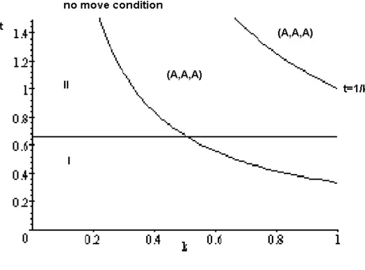
The sustainability of the agglomeration of allfirms in regionA is checked for all values of the parameters k and t, considering t in ascending order. Two main regions in the parameters space are considered: region I, where
the downstream firms located in A can export to B, because the transport costs are low; and region II, where the exports by downstream firms located in A are not feasible.
Region I is further subdivided according to the markets where a moving downstream firm located in B is active. In subregion I.1, the moving down-streamfirm located inB is active in both markets because the transport cost is low. In subregion I.2, the moving firm can sell only in its local market, although the firm located in A can sell in both markets. In subregion I.3, each downstream firm can sell only in its local market.
Region II is also subdivided. In subregion II.1, the moving downstream
firm located inB can import the intermediate good and produces a positive output. In subregion II.2, the transport cost of the input is too high and the downstreamfirm located in B is unable to produce.
Wefirst consider the case where the downstreamfirms are active not only in market A but also in market B. Their profit functions in the third stage are:
π1(A, A, A) = (1−(q1a+q2a)−wa)q1a+ [1−(q1b+q2b)−wa−t]q1b
π2(A, A, A) = (1−(q1a+q2a)−wa)q2a+ [1−(q1b+q2b)−wa−t]q2b (1)
where q1a, q2a, q1b, q2b are the quantities sold by firms 1 and 2 in markets A and B and wa is the delivered price of the input regionA.
Maximizing the profit functions in relation to the quantities, we obtain the outputs in each market.
q1∗a = q2∗a=
1
3(1−wa) (2)
q1∗b = q2∗b =
1
3(1−wa−t)
The derived demand of the input in region A is
xa =q1∗a+q2∗a+q∗1b+q∗2b
The profit function of the upstream firm is
π3 =waxa
If this profit function is maximized in relation towa, we obtain
w∗a=
1 2−
1
Substitutingwa into 2, we obtain
q1∗a = q2∗a=
1 6 +
1
12t (4)
q1∗b = q2∗b =
1 6 −
1 4t
The condition of an interior equilibrium (region I) where both firms are active in markets A andB is
q1∗b =q2∗b >0⇔t <
2
3 (5)
If we substitute quantities 4 and input price 3 in the profit functions of the downstream firms 1, we obtain:
π∗1(A, A, A) =π∗2(A, A, A) = 1 18 −
1 18t+
5 72t
2
(6)
On the other hand, if t > 23, we have a corner solution (region II) where the downstreamfirms located in A do not export to regionB, so that
q1∗b =q2∗b = 0
In this case, the profit functions of the consumer goods firms are
π1 = (1−(q1a+q2a)−wa)q1a (7)
π2 = (1−(q1a+q2a)−wa)q2a
Maximizing these profit functions, we obtain the optimal outputs
q1∗a =q2∗a=
1
3(1−wa) (8a)
The derived demand of the intermediate good in regionA is
xa =q1∗a+q2∗a
The profit function of the upstream firm is
π3 =waxa
Maximizing this profit function with relation to the input price, we obtain
w∗a=
1
Substituting this price of the intermediate good in 8a, the profit maxi-mizing quantities of the downstream firms are:
q1∗a =q2∗a=
1 6
Substituting these quantities and input price 9 in profit functions 7, we obtain the profits of the downstreamfirms in equilibrium:
π∗1(A, A, A) =π∗2(A, A, A) = 1
36 (10)
Figure 1 plots the regions where the interior solution (region I) and the corner solution (region II) hold.
In order to assess whether or not there exists an agglomerated equilibrium
(A, A, A), we consider a move of a downstream firm (firm 2 w.l.g.) to region
B. The profitability of this move is evaluated for different levels of the parameters k andt. We consider the values of t in ascending order.
In region I of Figure 1, if t is low, the moving consumer goods firm is able to sell in both regions. This corresponds to subregion I.1. The profit functions of the downstreamfirms are
π1(A, B, A) = (1−(q1a+q2a)−wa)q1a+ [1−(q1b+q2b)−wa−t]q1b
π2(A, B, A) = (1−(q1a+q2a)−wb−t)q2a+ [1−(q1b+q2b)−wb]q2b (11)
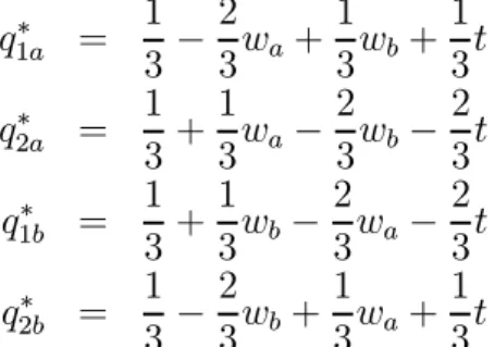
where wb is the delivered price of the input in region B. The profit maxi-mizing quantities are
q1∗a =
1 3 −
2 3wa+
1 3wb+
1
3t (12)
q2∗a =
1 3 +
1 3wa−
2 3wb−
2 3t
q1∗b =
1 3 +
1 3wb−
2 3wa−
2 3t
q2∗b =
1 3 −
2 3wb+
1 3wa+
The derived demands of the input in regions A andB are
xa = q1∗a+q1∗b
xb = q2∗a+q2∗b
The profit function of the upstream firm is
π3 =waxa+ (wb−kt)xb
If this profit function is maximized in order to the input prices, we can obtain these as:
w∗a =
1 2−
1
4t (13)
w∗b =
1 2−
1 4t+
1 2kt
Plugging these input prices into quantities 12, these become
q1∗a =
1 6 +
5 12t+
1
6kt (14)
q2∗a =
1 6 −
7 12t−
1 3kt
q1∗b =
1 6 −
7 12t+
1 6kt
q2∗b =
1 6 +
5 12t−
1 3kt
A sufficient condition for all the quantities to be positive is thatq2∗a >0. If this condition is met, the firm in region B imports the intermediate good from region A and is able to sell the consumer good in this region. The condition that defines subregion I.1 is
q2∗a >0⇔t <
2
7 + 4k (15)
If we substitute outputs 14 and input prices 13 in the profit function of
firm 2 in 11, this profit becomes
π2(A, B, A) = µ1
6 − 7 12t−
1 3kt ¶2 + µ1 6 − 1 3kt+
5 12t
¶2
(16)
Putting together 6 and 16, we can solve the inequality
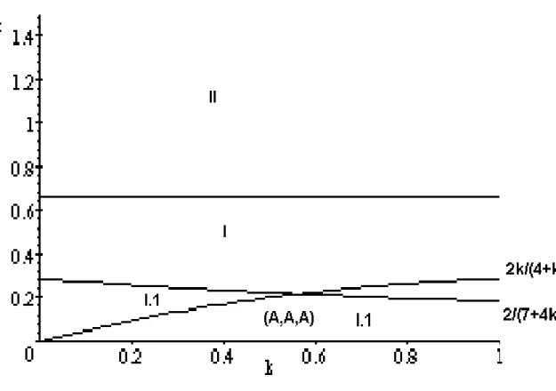
Figure 2: Existence of an agglomerated equilibrium in subregion I.1
which can be shown to mean that
0< t < 2k
4 +k+ 2k2 (17)
In Figure 2, we plot together the lines t = 2
7 + 4k (from 15) and t = 2 3
(from 5). We also plot the condition of the non-profitability of a change of
location by firm 2, t < 2k
4 +k+k2 (from 17), thus defining the region where (A, A, A) is an equilibrium of locations.
the ratio between the transport costs of the intermediate good and of the
final good k is higher than a threshold (≈ 0.56). If k is smaller than this threshold, agglomeration in Ais a location equilibrium if the general level of transport costs t is low.
If t > 2
7 + 4k, the output sold by firm 2 in regionA is zero. We assume
that the output sold by firm 1 in market B is positive, q1b > 0, and the economy is in subregion I.2. The profit functions of the downstream firms are:
π1(A, B, A) = (1−(q1a+q2a)−wa)q1a+ [1−(q1b+q2b)−wa−t]q1b
π2(A, B, A) = (1−(q1b+q2b)−wb)q2b (18)
The profit-maximizing outputs of the downstreamfirms are:
q1a =
1 2 −
1
2wa (19)
q1b =
1 3 +
1 3wb−
2 3wa−
2 3t
q2b =
1 3 −
2 3wb+
1 3wa+
1 3t
The derived demands of the input in regions A andB is:
xa = q1a+q1b
xb = q2b
The profit function of the upstream firm is
π3 =waxa+ (wb−kt)xb
Maximizing this profit function, the profit-maximizing delivered prices of intermediate goods for the upstreamfirm in both regions are:
wa =
1 2−
1
4t (20)
wb =
1 2+
1 8t+
Substituting wa and wb in the quantities produced by the downstream
firms, we obtain
q1∗a =
1 4 +
1
8t (21)
q1∗b =
1 6 −
11 24t+
1 6kt
q2∗b =
1 6 +
1 6t−
1 3kt
The border conditionq∗1b >0is equivalent to
t < 4
11−4k (22)
Substitutingq∗1b, q∗2b from 21 andwb from 20 in the profit function offirm 2 in 18, we obtain the profit of firm 2 in terms of the parameters:
π2(A, B, A) = µ1
6 + 1 6t−
1 3kt
¶2
(23)
From 6 and 23, it is possible to write the condition of the non-profitability of a move from region A to region B byfirm 2 as
π2(A, A, A)>π2(A, B, A)
It is easily seen that this condition holds for any values oft if 1
4 < k <1.
For k < 1
4, the condition is satisfied if
t < 1
2 (−3−8k+ 8k2) ³
−8 + 8k+ 2√10−48k+ 32k2´ (24)
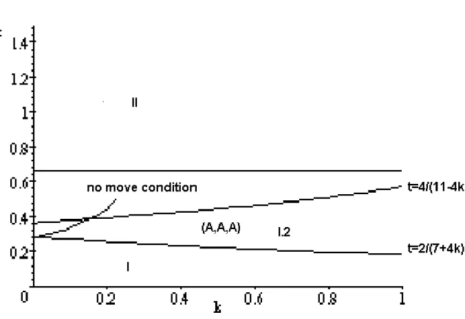
The border conditions defining region I.2., as given by t > 2
7+4k (the opposite of 15) and 22, are plotted in Figure 3. In this figure, the condition 24 of the non-profitability of a move from region A to region B by firm 2 is also plotted, defining the region where (A, A, A) is an equilibrium of locations.
In subregion I.3, althought < 2
3, transport costs are high enough so that
each firm sells only in its local market, so that q2a = q1b = 0. Hence the profit functions of the downstream firms are
π1(A, B, A) = (1−q1a−wa)q1a (25)
The profit-maximizing outputs are
q1a =
1 2 −
1
2wa (26)
q2b =
1 2 −
1 2wb
The derived demand of the input in each region is given by
xa = q1a
xb = q2b
The profit function of the upstream firm is given by
π3 =waxa+ (wb−kt)xb
Maximizing this profit function, we obtain the optimal delivered prices of the intermediate good in each region.
wa =
1
2 (27)
wb =
1 2+
1 2kt
Plugging these input prices into 26, these outputs become
q1∗a =
1
4 (28)
q2∗b =
1 4 −
1 4t
It is easy to see that the condition q∗2b > 0 ⇔ t <
1
k is always met in region I.3., where t < 2
3 holds. Substituting the input price wb from 27 and
the output q2∗b from 28 in the profit function of firm 2, as given by 25, we obtain the profit of firm 2 in terms of the parameters.
π2(A, B, A) = µ1 4 − 1 4kt ¶2 (29)
This profit can be compared with the profit that firm 2 obtains in the agglomeration, given by 6, in order to derive the condition of the non-profitability of a move by this firm.
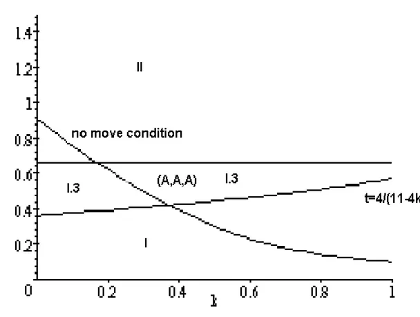
Figure 4: Existence of an agglomerated equilibrium in subregion I.3
It is easy to see that this condition is met if and only if
t > 1 2 (−10 + 9k2)
³
−8 + 18k−2√26−72k+ 72k2´ (30)
In Figure 4, we plot the border conditions given byt > 11−44k(the opposite of 15) and by t < 23. The condition of the non-profitability of a move byfirm 2, given by 30, is also plotted, thus defining the region where (A, A, A) is a locational equilibrium.
We now consider region II witht > 2
3, where thefirms agglomerated inA
only sell in their home market. In this case, we have to consider two different subregions. In the first subregion, labelled II.1., t < 1
Figure 5: Existence of an agglomerated equilibrium in region II.
As the profit of firm 2 when it is agglomerated in region A is given by 10, the condition of the non-profitability of a change of location
π2(A, A, A)>π2(A, B, A)
can be shown to mean that
t > 1
3k (31)
In Figure 5, we plot the border conditionst > 2 3, t <
1
k and the condition of the non-profitability of a change of location given by 31, thus defining the region where (A, A, A)is a locational equilibrium.
In subregion II.2, where t > 1
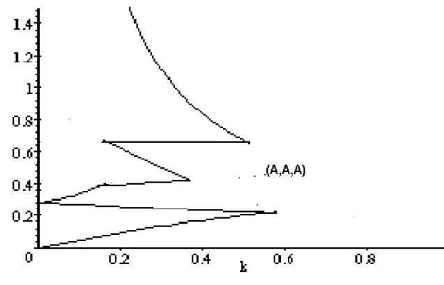
Figure 6: Existence of an agglomerated equilibrium in the space of parame-ters (k, t)
transport costs of the intermediate good produced in region A. Hence, in this subregion,(A, A, A) is a locational equilibrium as shown in Figure 5.
In Figure 6, we superimpose all the previous figures in order to obtain a representation of the region of the space of parameters where the agglomer-ation of the three firms in regionA is a subgame perfect equilibrium of the three-stage game.
3
Concluding remarks
The first unsurprising conclusion is that the region where the agglomerated equilibrium holds expands as k increases. As the previous literature in this
field has shown, if the transport cost of intermediate goods is high in relation to the transport cost of final goods, the firms that produce the final goods have no incentive to leave the location where the input is supplied. The second and more personal conclusion is that, for relatively low values ofk, the existence of an agglomerated equilibrium varies non-monotonically with the overall level of transport costs. This nonmonotonic pattern derives from the fact that the increase in transport costs has two opposing effects. An increase in the transport cost of the intermediate good creates an incentive for the upstream and downstream firms to cluster. But an increase in the transport cost of the consumer good leads downstreamfirms to become geographically isolated in order to relax intra-regional competition and cater for the local consumers in each region. This pattern is a generalization of the ”U inverted” pattern by KRUGMAN and VENABLES (1995) and VENABLES (1996) and it yields the well known conclusion that agglomeration occurs if transport costs are low in the specific case where each firm is active in each market.
This analysis could be extended by considering that the location decisions of firms change the production costs related with the primary factors of production in each region. With this generalization, it would be necessary to check the non-profitability of a move by the input supplier away from the agglomeration, since a locational shift could reduce its production costs, although it would entail additional transport costs of the intermediate good.
References
AMITI, Mary (2001), ”Regional specialization and technological leapfrogging”, Journal of Regional Science, vol. 41, pp. 149-172.
BELLEFLAMME, Paul and Eric TOULEMONDE (2003), ”Product differentiation in successive vertical oligopolies”, Canadian Journal of Economics, vol. 36, pp. 523-545.
FUJITA, Masahisa and Jacques-François Thisse (2002), Economies of Agglomeration — Cities, Industrial Location and Regional Growth, Cam-bridge, Cambridge University Press.
KOOPMANS, Tjalling and Martin BECKMANN (1957), ”Assignment problems and the location of economic activities”, Econometrica, vol. 25, pp. 53-76.
KRUGMAN, Paul and Anthony VENABLES (1995), ”Globalization and the inequality of nations”, Quarterly Journal of Economics, vol. 110, pp. 857-880.
MARSHALL, Alfred (1890), Principles of Economics, London, Macmillan, 8th ed., published in 1920.
PONTES, José Pedro (2003), ”Industrial clusters and peripheral ar-eas”, Environment and Planning A, vol. 35, pp. 2053-2068.