Universidade de Brasília
FACULDADE DE ECONOMIA, ADMINISTRAÇÃO E CONTABILIDADE
DEPARTAMENTO DE ECONOMIA
LUCAS EDUARDO VERAS COSTA
COMMODITY PRICES IN BRAZIL: FISCAL POLICY, INTEREST
RATES AND SECTORIAL IMPACTS
BRASÍLIA
2019
Universidade de Brasília
FACULDADE DE ECONOMIA, ADMINISTRAÇÃO E CONTABILIDADE
DEPARTAMENTO DE ECONOMIA
LUCAS EDUARDO VERAS COSTA
COMMODITY PRICES IN BRAZIL: FISCAL POLICY, INTEREST
RATES AND SECTORAL IMPACTS
Dissertação apresentada ao curso de Mestrado Acadêmico em Economia da Universidade de Brasília – UnB, como requisito para a obtenção do título de Mestre em Economia.
Orientadora: Prof. Dra Marina Delmondes de Carvalho Rossi
BRASÍLIA
2019
Resumo
Os preços das commodities podem afetar a economia brasileira por meio de um processo multifacetado. Este artigo analisa como o ciclo de preços das commodities afeta o Brasil, através da visão de três variáveis macroeconômicas: (a) Política Fiscal, (b) Taxa de Juros, (c) Valor Agregado Setorial. Estimando modelos lineares e modelos auto-regressivos vetoriais, os resultados sugerem que a receita do governo está ciclicamente alinhada com os preços das commodities, o risco-país diminui quando os preços das commodities estão altos e um aumento nos preços das commodities impacta positivamente não apenas o setor de commodities, mas também o setor industrial e de serviços.
Palavras-chave: Ciclos de Negócios, Preços de Commodities, Risco País, Política Fiscal,
Abstract
Commodity prices might affect the Brazilian economy through a multifaceted process. This paper analyzes how commodity prices cycle affects Brazil through the lens of three macroeconomic variables: (a) Fiscal Policy, (b) Interest Rate, (c) Sectorial Aggregate Value. Estimating linear models and Vector Auto-Regressive models, the results suggest that government revenue is cyclically aligned with commodity prices, country risk reduces when commodity prices are high, and a rise on commodity prices impacts positively not only the commodity sector, but also the industrial and service sector.
Keywords: Business Cycles, Commodity Prices, Country Risk, Fiscal Policy, Sectorial
Summary
1 Introduction __________________________________________________________ 7
2 Relates Literature ______________________________________________________ 9
3 Real Commodity Prices Index ___________________________________________ 12
4 Fiscal Policy __________________________________________________________ 14
4.1 Fiscal Policy and Commodity Prices Cyclicality _________________________________ 15 4.2 Fiscal Policy and Commodity Prices Shocks ___________________________________ 20
5 Interest Rates ________________________________________________________ 24
5.1 Country Spreads and Commodity Prices Cyclicality _____________________________ 26 5.2 Country Spreads and Commodity Prices Shocks _______________________________ 28
6 Sectoral Impacts ______________________________________________________ 32
6.1 Commodity Prices shock on Brazilian Sectors _________________________________ 34
7 Concluding Remarks __________________________________________________ 40
8 References ___________________________________________________________ 43
9 Appendix ____________________________________________________________ 47
9.1 Data Sources____________________________________________________________ 47 9.2 List of Abbreviations _____________________________________________________ 47 9.3 Share of Commodity Products on the Commoditty Index ________________________ 48 9.4 Evolution of Commoditty Imports and Commodity Exports ______________________ 49 9.5 The Voracity Effect _______________________________________________________ 50 9.6 Other Regression for brazil Country Spread ___________________________________ 53
List of Figures
Figure 1 - Commodity Prices and Brazil Co-movements ... 7
Figure 2 - Commodity Prices Index ... 13
Figure 3 - Brazil Real Central Government Revenues (R$ millions) and Commodity Prices 14 Figure 4 - Brazil Real Central Government Expenses (R$ Millions) and Commodity Prices 15 Figure 5 - Impulse Response of Fiscal Variables to One Standard Cholesky Innovation in Commodity Prices (In Percent) ... 21
Figure 6 - Impulse Response of Fiscal Variables to One Standard Cholesky Innovation in Commodity Prices (In Percent) ... 22
Figure 7 - Interest Rates and Commodity Prices ... 25
Figure 8 - Impulse Response Function to a one standard deviation shock in commodity prices ... 29
Figure 9 - Accumulated Impulse Response Function to a one standard deviation shock in commodity prices ... 30
Figure 10 - Sectorial Added Values (R$ Millions) ... 32
Figure 11 - Share on Aggregated Added Value ... 33
... 33
Figure 12 - Commodity exports (% as share of total exports) ... 34
Figure 13 - Impulse Response Function to a one standard deviation shock in commodity prices (sectorial analysis) ... 35
Figure 14 - Accumulated Impulse Response Function to a one standard deviation shock in commodity prices (sectorial analysis) ... 36
Figure 15 - Impulse Response Function to a one standard deviation shock from world GDP 37 Figure 16 - Accumulated Impulse Response Function to a one standard deviation shock from world GDP... 37
Figure 17 - Commodity Exports as Share of Total Exports (%) ... 49 Figure 18 - Commodity Imports as share of Total Imports (%) ... 49 Figure 19 - Iron Ore, Soybeans and Crude Oil as Share of Total Commodities
List of Tables
Table 1 - Fiscal Variables Regressions ______________________________________ 16 Table 2 - Fiscal Variables Regressions ______________________________________ 18 Table 3 - Fiscal Variables Regressions ______________________________________ 18 Table 4 - Fiscal Variables Regressions ______________________________________ 20 Table 5 - Variance Decomposition of Forecast Errors (In Percent) ______________ 23 Table 6 - Real Spread Regressions (using UK interest rate) ____________________ 27 Table 7 - Real Spread Regressions (using US interest rate) _____________________ 27 Table 8 - Variance Decomposition of Forecast Errors _________________________ 31 Table 9 - Forecast Error Variance Decomposition from Commodity Prices (Sectorial Analysis) 38
Table 10 - Forecast Error Variance Decomposition from Real World GDP (Sectorial Analysis) 38
Table 11 - Commodity Prices Weight ______________________________________ 48
Table 12 - Country Spreads Regressions (UK Real Money Market Rate) ________ 53
Table 13 - Country Spreads Regressions (UK Real Saving Rate) _______________ 53
1 Introduction
Commodities prices are important triggers of business cycles on emerging economies,
as stated by Fernadez et al. (2017) and Dreschell and Tenreyro (2018). In general, either those countries depend on the revenues of commodity exports or their economy depends on the imports of those commodities, such as food and oil, so that their economies can work properly (UNCTAD, 2017). IMF (2019) also stressed the role of commodity prices to forecast economic activity. According to them, the commodity prices contain rich information about the current state of the emerging economies. From 1997 to 2017, Brazil´s commodity exports represented only 30 % of total exports and, additionally, commodity imports was only 13% of Brazil total imports, which makes Brazil a non-commodity dependent country1. However, Brazil’s output
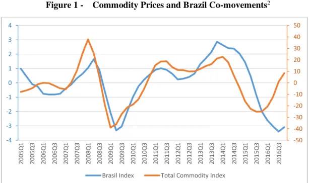
had strong co-movements with the commodity prices as shown in Figure 1. Since commodity prices might affect the Brazilian economy through a multifaceted process, this research analyzes the impacts of the commodity prices empirically, through the lens of three macroeconomics variables: (1) the fiscal policy, (2) the interest rates and (3) the sectorial aggregated value.
Figure 1 - Commodity Prices and Brazil Co-movements2
Source: IMF, Author’s Elaboration
1 According to UNCTAD (2017) classification
2 The chart shows the quarterly cyclical components of the real commodity index and Brazil
gdp index (2010 =100). The cyclical component was obtained with the HP filter with frequency = 1600. The right vertical axe indicates the deviation from trend for Real Commodity Index and left vertical axe indicates the deviation from trend for Brazil’s gdp index.
-50 -40 -30 -20 -10 0 10 20 30 40 50 -4 -3 -2 -1 0 1 2 3 4 20 05 Q 1 20 05 Q 3 20 06 Q 1 20 06 Q 3 20 07 Q 1 20 07 Q 3 20 08 Q 1 20 08 Q 3 20 09 Q 1 20 09 Q 3 20 10 Q 1 20 10 Q 3 20 11 Q 1 20 11 Q 3 20 12 Q 1 20 12 Q 3 20 13 Q 1 20 13 Q 3 20 14 Q 1 20 14 Q 3 20 15 Q 1 20 15 Q 3 20 16 Q 1 20 16 Q 3
I analyze how the commodity prices impacts Brazil´s fiscal policy using two methodologies. First, I examine the cyclicality of selected fiscal variables with the commodity prices, through the estimation of OLS equations. The results show that tax and central government revenues are contemporaneous cyclical with the commodity prices while total and personnel expenditures are cyclical with the lag of commodity prices cyclical component. Second, I run a Vector Auto-Regressive Model (VAR) including Commodity Prices, Government Revenues and Government Expenditure. The impulse response functions show that a positive shock to commodity prices makes the government revenues grow while its impact on the government spending is nearly zero.
The impact on interest rates was analyzed by first checking how the commodity prices impact the spread between the domestic interest rate and the international interest rate, using ordinary least squares equations and controlling by output growth, trade balance, and debt. If we consider that the country spread reflects the financial conditions of the country, a commodity prices shock can aid or deteriorate its situation. The result points out that there is a significant and negative correlation between commodity prices and Brazil’s interest rate spread. The second approach was to estimate a VAR including commodity prices, country interest rate spread, output, trade balance, real credit to the non-financial sector, and real exchange rate. The results corroborates that commodity prices shock reduces the country spread, accelerates the rate of growth of the output, and augment the credit to the non-financial sector, as expected. However, exchange rate appreciates and trade balance deteriorates, which can be explained by the entrance of foreign capital in time of commodity booms. Moreover, this model estimates that commodity prices contribute to 26% of Brazil output fluctuation.
The last approach focus on the impact of commodity prices on Brazilian aggregate value. I run a VAR dividing the Brazilian economy on commodity, industrial and services sector. I allow for two international shocks on the model; a shock to global demand and a shock to commodity prices. One would expect that a rise on the commodity prices would imply a cost to the service and industrial sectors. However, the impulse response functions of this model reveals that a positive shock to commodity prices raises the growth of the services and industrial sectors.
I structure the rest of this research as follows: Section 2 presents the related literature, Section 3 presents how the Brazilian real commodity prices index was constructed, Section 4 analyzes the impacts on Brazil fiscal policy, Section 5 on the interest rate, and Section 6 on Brazil sectorial added value. Section 7 concludes the research.
2 Related Literature
There is a branch of literature that focus on the negative relationship between commodity prices and domestic interest rates. Dreschell and Tenreyro (2018) study the relationship between commodity prices and countries interest rates spreads. They run an OLS regression of countries´ spread and commodity prices deviation from its long run trend. They find that a 10% deviation of the commodity prices from their long run trend allows the spread between Argentina interest rate and international interest rate to reduce about 2%. I run a similar model on this research; however, I focus on the growth of commodity prices and Brazil’s interest rate spread. Additionally, they develop a DSGE model exploring this relationship. On a similar line, Fernandez et al. (2015) emphasize a negative correlation between commodities prices and sovereign bonds spreads for emerging economies. When commodity prices are high, these economies have access to cheaper foreign credit. Uribe and Yue (2006) analyze the impact of country spread and US interest rate for a set of emerging countries, they find that the US interest rate and the country risk are the main drivers of the business cycles on those countries. Shousha (2016) uses a panel VAR methodology across emerging and developed countries that are commodity dependent exporters. He finds that negative correlation between commodity prices and the domestic interest rate is one of the main differences between emerging and developed countries. I run a similar model on this research. However, I focus on a VAR model using only Brazilian domestic variables.
Bastourre et al (2012) estimate the correlation between a common factor of the returns on emerging economy bonds and a common factor of commodity prices. They find this correlation to be -0.81, which emphasizes a strong negative correlation. Neumeyer and Perri (2005) find that for a sample of developing countries the interest rate is countercyclical and it is responsible for leading the cycle. They also develop a model including a country risk component, which is responsible, according to the authors, for amplifying shocks of fundamental variables.
The literature also focuses on the co-movements between fiscal policy and commodity prices. I base my analysis on Cespedes and Velascos (2014), who study this cyclicality on two episodes for a set of developing and developed countries. The first episode is in the 1970’s and 1980’s boom, and the second episode is the commodity prices boom right before the 2008 crisis. They find that in the first episode, the developing countries were pro-cyclical or a-cyclical. However, during the second episode, the government expenditure remained relatively stable
during the commodity boom. I update their analysis focusing on the period from 1997 to 2017 for Brazil.
Boccara (1990) notes that countries that face a windfall in government revenues, especially commodity exporters, tend not to act accordingly to the permanent income hypothesis. Instead, the windfall is used to increase the levels of government consumption and to finance ambitious investment projects. He cites three major reasons. First, those governments face a pressure to spend. In countries where exists a lot of unmet needs, special interest groups and government agencies may pressure the government to spend immediately the excess of wealth generated by the revenues surplus. Second, during the increase of the spending levels, the government usually invests on long-term investment projects or on expanding the public labor force. These types of spending are difficult to reverse once it is made. Finally, at the onset of a commodity bust, the government is able to finance the higher level of spending as long as the fiscal rules allow him and financing is available. As a result, the public debt tends to raise. Villafuerte and Murphy (2010) study the behavior of 31 oil-producing countries during the 2003-2008 oil price cycle. They find that those countries have a pro-cyclical fiscal policy, which exacerbated the fluctuation on the economic activity. Interestingly, they also concluded that an increase on the spending, during this cycle, significantly worsened their non-oil primary balance.
Similarly, Erbil (2011) analyzes the cyclical behavior of 28 developing oil-producing countries during 1990-2009, using five fiscal variables, government expenditure, consumption, investment, non-oil revenue and non-oil primary balance. He finds that the fiscal policy was pro-cyclical throughout the entire sample. Some of his evidence suggests that high political quality and better institutional factors contribute to reduce this cyclicality.
Medina (2016) analyzes the dynamic effect of commodity prices fluctuations on fiscal revenues and spending for 8 Latin American countries. He estimates a VAR and finds finds that the fiscal position for those countries responds to a shock to commodity prices, however, the magnitude of these responses is heterogeneous among the countries. He atributes this distinct behavior among those countries to institutional arrangements, which in some cases include the efficient use of fiscal rule to enforce political commitment and high standards of transparency.
Moving on to sectorial impacts of commodity prices, Naizloglu and Soytas (2011) study the effect of oil prices on agricultural prices in Turkey. They argue that it might have two type of effects, one direct, and one indirect, through the exchange rate channel. To analyze this issue,
they used a VAR, employing a method developed by Toda and Yamamoto (1995) to do a long-run Granger causality test and. They then computed the generalized impulse-response functions. Surprisingly, they find that the oil prices have no significantly impact on agricultural prices, neither through the direct effect nor through the indirect effect.
Beghold, Larsen and Seneca (2017) study the impact of oil prices shocks on the Norwegian economy, which is highly dependent on oil exports. They run a Vector Auto-Regressive Model, identifying the impacts of global demand and international oil price on the oil and non-oil sector in Norway. Similar to my results, they find that a shock to commodity prices does not crowd out the non-commodity sector.
Some authors also study the impact of commodity prices on Brazil. Melo (2013) examines the pass-through mechanisms of commodity prices to the consumer inflation. He develops a commodity price index, designed specifically for Brazil, using the VAR methodology to compute the coefficients of how each commodity price affects the Brazilian consumer price index. He finds that the commodity prices significantly affected the consumer price index from 2009-2012 in Brazil, even though it did not affect it from 2006-2009. The rise of commodity prices from 2009-2011 increased Brazilian inflation, although it was smoothed by the exchange rate appreciation. However, the decline of commodity prices in 2011-2012 allowed Brazil's inflation to be at a lower level.
Bredow, Lélis and Cunha (2016) study the influences that the cycle of high commodities prices had in the Brazilian economy, especially on the foreign capital inflows. They used a Markov switching method and the Vector Error Correction Model to achieve this goal. They find that the rise of exports and foreign domestic investment occurred at the same moment of the rise of the commodities price and that this rise influenced the foreign capital entrance in Brazil, particularly in the overseas sales of goods and in the short term of financial flows.
3 Real Commodity Prices Index
Many institutions offer a commodity prices index, such as the IMF, World Bank and ECLAC. However, they use different sources of primary data on commodity products and different shares for each commodity on their final index. Those indexes might not exactly reflect the importance of the commodity prices for a specific developing country.
To deal with this issue, I apply the procedure pioneered by Grilli and Yang (1988) and implemented in more detail by Pfaffenzeller et al (2007). I use the World Bank commodity price database, called the “Pink Sheet”. 3 For each commodity product, I obtain a quarterly price
by averaging the three months prices. I focus on the period of 1996 to 2017, which are the years of the empirical analysis. I then obtain the commodity prices weight of each product using the UN Comtrade database of Brazil exports during 1996-2017. I use a Laspeyeres index as defined below:
𝐶𝑃𝐼𝑡 = ∑𝑛𝑖=1𝛼𝑖𝑃𝑖,𝑡,
in which, CPI is the commodity price index in question, n = 34, and accounts for all commodities available in the World Bank database for commodity prices. 𝑃𝑖,𝑡 accounts for commodity price 𝑖 in the period 𝑡. This database sometimes offers multiples prices (from different sources for the same commodity). In those cases, I compute a simple average of the available prices of those commodities. The weight of each commodity,𝛼𝑖, is its share of commodity product 𝑖 on all commodity exports for the analyzed period. In the context of a small open economy, those prices tend to be a good proxy for the international price and they are relevant to explain how shocks to commodity prices affect Brazil.
The products with the highest share are: Iron Ore (23.6 %), Soybeans (17.8 %) and Crude Oil (14,72%). Altogether, they represent 56.1% of all value share. However, this was not always the case throughout the period. The share of this basket represented only 29% of the total commodity exports in 1995, however, it jumps to 50% in 2006 and it peaks to 61% in 2011. 4
I use a fixed weight for each commodity price because the use of a varying weight would bring too much noise to the data and, thus, it would prevent us from identifying relevant cycles of the commodity prices for Brazil's economy. After the construction of the index, I deflate it
3 Database available in http://www.worldbank.org/en/research/commodity-markets 4 The share of each commodity to the real commodity index is available on the appendix.
using the producer price index for the United States. The figure below shows the deviation from mean5 of Brazil Commodity Prices and a comparison between Brazil specific Commodity
Prices and the World Commodity Prices provided by IMF.
Figure 2 - Commodity Prices Index
Source: World Bank, IMF. Author’s Elaboration
The figure shows that World Commodity Price and Brazilian specific followed a similar path from 1995 to 2017. The commodity prices had a strong cycle during the 2008 world crisis, accelerating sharply before the crisis, and then, facing a strong downfall. In 2015, it faced another great downfall, which coincides with the beginning of Brazil´s recession period.
5 I obtain the deviation from mean through the application of HP-filter with frequency 1600.
-0.4 -0.3 -0.2 -0.1 0 0.1 0.2 0.3 0.4 1995Q 1 1996Q 1 19 97 Q 1 1998Q 1 1999Q 1 2000Q 1 2001Q 1 2002Q 1 2003Q 1 2004Q 1 2005Q 1 2006Q 1 2007Q 1 2008Q 1 2009Q 1 2010Q 1 2011Q 1 2012Q 1 2013Q 1 2014Q 1 2015Q 1 2016Q 1 2017Q 1
Brazil Commodity Prices (Deviation from mean) 0 20 40 60 80 100 120 140 160 1995Q 1 1996Q 1 1997Q 1 1998Q 1 1999Q 1 2000Q 1 2001Q 1 2002Q 1 2003Q 1 2004Q 1 2005Q 1 2006Q 1 2007Q 1 2008Q 1 2009Q 1 2010Q 1 2011Q 1 20 12 Q 1 2013Q 1 2014Q 1 2015Q 1 2016Q 1 2017Q 1
Brazil vs World Commodity Prices (2010 =100)
Brazil Commodity Prices World Commodity Price Index
4 Fiscal Policy
The literature focuses on the role that fiscal rules have to reduce the pro-cyclicality of the fiscal policy on emerging markets. Brazil´s fiscal rule, in sum, consists on a golden rule (which prohibits credit operations that exceed capital expenses) and a set of measures defined by the Fiscal Responsibility Law.The fiscal framework imposes that the legislative house approves a fiscal target of revenues, expenditures, primary, and nominal surplus to be pursued by the executive during the following year. A branch of literature confirms that this fiscal rule improved fiscal discipline of the federal and subnational governments. 6
However, Brazilian national accounts had deteriorated on the last 3 years despite the presence of this fiscal rule. 7 We note that the revenues of the central government have
significant co-movements with the real commodity prices index, as Figure 3 shows. Along with the accelerations of the commodity prices, government revenues have grown, allowing government expenditures to increase without deteriorating the primary surplus. After the 2008 crisis, the commodity prices accelerated, as so the government expenditures, the latter even more as the government pursued anti-cyclical policies through fiscal stimulus.
Figure 3 - Brazil Real Central Government Revenues (R$ millions) and Commodity Prices
Source: Brazil National Treasury Secretary. Author’s Elaboration
6 See for example Luporini (2013), Caceres et al (2010) and Alston (2009).
7 In 2016, a federal law was approved, imposing a ceiling to real government expenses, in
attempt to contain this deterioration.
0 20 40 60 80 100 120 140 0 200000 400000 600000 800000 1000000 1200000 1400000 1600000 1800000
Figure 4 - Brazil Real Central Government Expenses (R$ Millions) and Commodity Prices8
Standard theory would predict that in times of a commodity boom, which would increase government revenues, the central planner would smooth its consumption by raising its fiscal surpluses and accumulating assets. However, if the government have multiples policy-makers trying to absorb this extra revenue to impose its own agenda, known as the voracity effect, a large share of the revenues from commodities is spent and consumption smoothing breaks down.9
It is vital to detect how the government revenues and expenditures respond to the fluctuations of the commodity price in order to determine its role on the deterioration of Brazil fiscal accounts. I analyze this issue empirically by applying two strategies. First, estimating ordinary least square equations and then estimating a VAR.
4.1 Fiscal Policy and Commodity Prices Cyclicality
In this section, I run the same regressions used in Cespedes and Velascos (2014), but restricting the analysis for Brazil10. The first regression is the following:
𝑑(𝑙𝑜𝑔𝐹𝑡) = 𝛼 + 𝛽𝑑(𝑙𝑜𝑔𝑃𝑡) + 𝜖𝑡,
8 Excluding social security expenses
9 For a formalization of the voracity effect, see the Appendix
10 Cespedes and Velasco (2014), run those regressions individually for each country and then average the
fiscal multiplier estimated around a set of commodity dependent country and industrialized countries.
0 20 40 60 80 100 120 140 0.00 200000.00 400000.00 600000.00 800000.00 1000000.00 1200000.00 19 97 19 98 19 99 20 00 20 01 20 02 20 03 20 04 20 05 20 06 20 07 20 08 20 09 20 10 20 11 20 12 20 13 20 14 20 15 20 16 20 17
Transfers Employees Remuneration Other Obligatory Expenses
in which 𝐹𝑡 is related to the following fiscal variables: (1) Total Revenues; (2) Tax Revenues;
(3) Total Spending (Excluding Social Security Spending)11; (4) Personnel Expenditures; (5)
Other Expenditures subject to financial programming. d(.) is the difference operator 𝑙𝑜𝑔𝑃𝑡 is the log of the commodity prices calculated as described in the Section 2, and 𝜀𝑡 is the error term.A positive sign for 𝛽 would indicate that the fiscal variable is cyclical with commodities prices. All the data came from Brazil National Treasury Secretary dataset, namely, Central Government Fiscal Results, and it is real and annually. This dataset is available from 1997-2018 which limits us to 21 observations. This strategy is the same used on Arreaza et al (1999). I also run a similar regression for the Fiscal Balance defined below:
𝐵𝑡 = 𝛼 + 𝛽𝑑(𝑙𝑜𝑔𝑃𝑡) + 𝜖𝑡,
in which 𝐵𝑡 is the primary surplus as percentage of GDP. Note that in this case, 𝛽 must be interpreted as semi-elastic coefficient. A positive value would suggest a pro-cyclicality with commodity prices. In this case, I am not interested in the elasticity of the fiscal variable with output, therefore, the omission of a variable of this kind is of minor significance in relation to endogeneity issues, since commodity prices are arguably exogenous to fiscal policy.
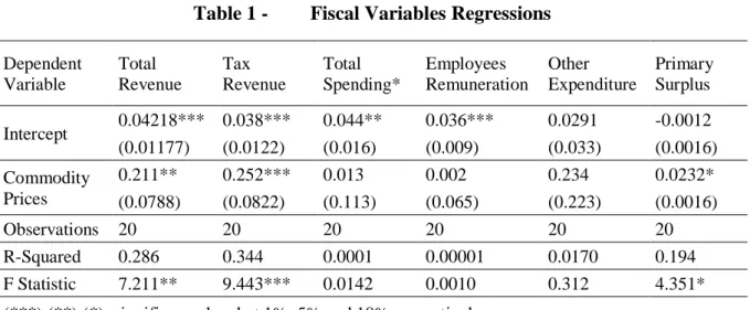
Table 1 - Fiscal Variables Regressions
Dependent Variable Total Revenue Tax Revenue Total Spending* Employees Remuneration Other Expenditure Primary Surplus Intercept 0.04218*** 0.038*** 0.044** 0.036*** 0.0291 -0.0012 (0.01177) (0.0122) (0.016) (0.009) (0.033) (0.0016) Commodity Prices 0.211** 0.252*** 0.013 0.002 0.234 0.0232* (0.0788) (0.0822) (0.113) (0.065) (0.223) (0.0016) Observations 20 20 20 20 20 20 R-Squared 0.286 0.344 0.0001 0.00001 0.0170 0.194 F Statistic 7.211** 9.443*** 0.0142 0.0010 0.312 4.351*
(***);(**);(*); significance level at 1%, 5% and 10% respectively.
Source: Author’s Elaboration
Table 1 summarizes the results. The equations related to government revenues and Primary Surplus are statistically significant, with the commodity prices coefficients positive and statistically significant. Those results suggest that an 1% increase in the commodity prices index increases the government revenues in 0.21%, and 0.25% for tax revenues. The results for
11 Social securities were excluded because they are obligatory expenditures not aligned with
the Brazilian cycle. Since I want to test cyclicality with commodity prices, in the low phase of the commodity cycle the government would be unable to adjust this expense.
the semi-elastic coefficient indicate that an increase in 1% for the commodity prices would augment the primary surplus, as percentage of GDP, in 0.02%. However, the equations for government spending are not statistically significant, neither the commodity prices coefficients, even though the latter is positive.
These results are quite intuitive, due to the fiscal programming of the government, spending should not be cyclical with commodity prices because they are defined before commodity windfall appears. However, fiscal revenues are obtained at the same time and so the commodity prices raise fiscal revenues for commodity products. These coefficients are quite different from the ones find in Cespedes and Velascos (2014), for 1996-2009 those authors identify that the coefficients for government revenues and spending are not statistically significant, those coefficients are and 0.01 and -0.15 respectively. They find that for the fiscal balance the coefficient is significant but quite larger from the one I found, 0.07.
The other strategy to estimate the fiscal cyclicality between fiscal policy and commodity prices relies on computing the cyclical component of the commodity prices index and fiscal variables. Gavin and Perrotti (1997) also uses this specification. In particular, I estimate the following equations by ordinary least squares:
𝐵𝑡= 𝛼 + 𝛽𝐶𝑡+ 𝜖𝑡
𝐵𝑡= 𝛼 + 𝛽𝐶𝑡+ 𝜃𝑌𝑡+ 𝜖𝑡.
In this case 𝐵𝑡 is the cyclical component of the fiscal variables, 𝐶𝑡 is the cyclical component of the commodities prices index and 𝑌𝑡 is the output gap.12 Both cyclical
components are in log of the deviation from the trend and are calculated by hp-filter, thus we are dealing with the elasticity of commodity prices cycle in relation to the fiscal variables cycle. I use the same set of fiscal variables of the previous exercise. By using the cyclical component of the commodity price index rather than the commodity prices itself, it is incorporated the transitory movements of the commodity prices. These movements might generate transitory revenues and the voracity effect may raise government spending. In this specification, a positive sign for 𝛽 indicates a pro-cyclicality between fiscal policy and commodity prices.
12The cyclical component of the commodity prices index and the fiscal variables are obtained
by applying a hp-filter with frequency equals to 500. The output gap is also obtained by applying a hp-filter on Brazil gdp.
Table 2 - Fiscal Variables Regressions Dependent Variable Total Revenue Tax Revenue Total Spending Personnel Expenditures Other Expenditure Primary Surplus Intercept 0.002 -0.001 0.0043 0.001 0.027 0.001 (0.009) (0.0119) (0.0196) (0.0100) (0.3951) (0.002) Commodity Prices 0.276 *** 0.201 *** 0.2134** 0.119** 1.205** 0.017 (0.045) (0.0584) (0.0959) (0.049) (0.525) (0.011) Observations 21 21 21 21 21 21 R-Squared 0.660 0.385 0.206 0.236 0.217 0.112 F Statistic 37.03*** 11.91*** 4.944** 5.876** 5.265** 2.417
(***);(**);(*); significance level at 1%, 5% and 10% respectively.
Source: Author’s Elaboration
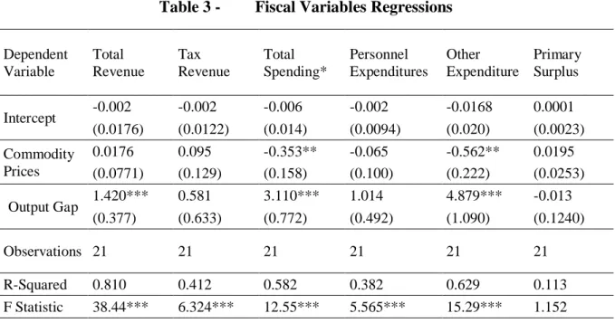
Table 3 - Fiscal Variables Regressions
Dependent Variable Total Revenue Tax Revenue Total Spending* Personnel Expenditures Other Expenditure Primary Surplus Intercept -0.002 -0.002 -0.006 -0.002 -0.0168 0.0001 (0.0176) (0.0122) (0.014) (0.0094) (0.020) (0.0023) Commodity Prices 0.0176 0.095 -0.353** -0.065 -0.562** 0.0195 (0.0771) (0.129) (0.158) (0.100) (0.222) (0.0253) Output Gap 1.420*** 0.581 3.110*** 1.014 4.879*** -0.013 (0.377) (0.633) (0.772) (0.492) (1.090) (0.1240) Observations 21 21 21 21 21 21 R-Squared 0.810 0.412 0.582 0.382 0.629 0.113 F Statistic 38.44*** 6.324*** 12.55*** 5.565*** 15.29*** 1.152
(***);(**);(*); significance level at 1%, 5% and 10% respectively.
Source: Author’s Elaboration
Table 2 and 3 summarize the results of the estimated regressions. When the output gap is omitted from the equations the results for government revenues are quite similar, with the coefficient associated with the commodities prices statistically significant and pro-cyclical. I consider this a great deal of evidence that government revenues are pro-cyclical with the commodity prices cycle. However, I cannot conclude the same for government spending. When we consider only the cyclical components of the commodity prices index and the government spending variables we see that the commodity prices coefficients became large, pro-cyclical, and statistically significant, nevertheless, when the output gap is introduced those variables
became counter-cyclical and statistically significant. This result is puzzling and it does not allow us to state whether the government spending is pro-cyclical, counter-cyclical or acyclical. In the case of the primary surplus, the analysis of its cyclical component might not be a reasonable one since its regressions lost statistical significance.
It may be that government spending does not co-move with contemporaneous commodity prices but rather with its lagged value. For example, suppose that in a year an increase in the commodity prices generates a windfall of revenues, the fiscal rule imposes that only the planned spending, approved in the legislative, is materialized. However, on the next year these new levels of revenues are taken into account in the spending planning for the next year, increasing the government spending. In order to test this proposition, I run the same regressions for the government spending variables, however, including the lag of the commodity prices variable. Specifically, the following equations are estimated by ordinary least squares:
𝑑(𝑙𝑜𝑔𝐹𝑡) = 𝛼 + 𝛽𝑑(𝑙𝑜𝑔𝑃𝑡−1) + 𝜖𝑡
𝐵𝑡 = 𝛼 + 𝛽𝐶𝑡−1+ 𝜖𝑡 𝐵𝑡= 𝛼 + 𝛽𝐶𝑡−1+ 𝜃𝑌𝑡+ 𝜖𝑡,
in which, d(.) is the differece operator, 𝐹𝑡 corresponds to government spending variables,
namely, Total Spending (Excluding Social Security Spending), Employees Remuneration; Other Expenditures subject to financial programming; 𝐵𝑡 is the cyclical component of those
fiscal variables, 𝑃𝑡−1 is the lag of the commodity prices index, 𝐶𝑡−1 is the lag of cyclical component of the commodity prices index, 𝑌𝑡 is the output gap and 𝜖𝑡 corresponds to the error
Table 4 - Fiscal Variables Regressions
Dependent Variable
Total Spending* Personnel Expenditures Other Expenditures
(1) (2) (3) (1) (2) (3) (1) (2) (3) Intercept 0.049*** -0.0035 -0.0030 0.0329*** -0.0035 -0.0041 0.031 -0.005 -.0079 (0.0117) (0.0112) (0.0114) (0.0097) (0.0112) (0.0160) (0.034) (0.0160) (0.0250) Lag Commodity Prices 0.0019 0.062 -0.142 (0.0771) (0.063) (0.228) Lag Commodity Prices Cycle 0.107*** 0.155 0.2077** 0.168 0.289 0.0341 (0.0556) (0.0983) (0.055) (0.137) (0.0792)** (0.214) Output Gap 0.3178 0.736 2.214 (0.490) (0.683) (1.069)** Observations 20 20 20 20 20 20 20 20 20 R-Squared 0.024 0.436 0.449 0.054 0.436 0.462 0.022 0.425 0.462 F Statistic 0.0001 13.92*** 6.947*** 0.972 13.92*** 7.312*** 0.387 13.34*** 7.317*** (***);(**);(*); significance level at 1%, 5% and 10% respectively.
Source: Author’s Elaboration
Table 4 summarizes the results of the estimations. We see that the coefficients for the lag of the commodity prices indicate a pro-cyclicality of government total spending and employees’ remuneration, however, only the equations that I include the cyclical component of the commodity prices and omit the output gap are indeed significant. It remains puzzling why the government expenditures are pro-cyclical commodity prices deviation from the trend and not with the log of the growth.
In sum, the results suggest that government revenues are contemporaneously cyclical with the commodity prices and the government expenditures are cyclical with the deviation from the trend of the lag of the commodity prices cycle.
4.2 Fiscal Policy and Commodity Prices Shocks
In the previous exercises, I did not identify the dynamic effects that a shock to commodity prices might have on the fiscal variables. In order to capture those effects, I estimate a VAR, similar to the one used in Medina (2010). The advantage of this method is that we can estimate the effect of a shock to commodity prices periods ahead and we can also evaluate the direct and indirect effects of the shocks (through their effect on GDP). Moreover, variance decomposition of forecast errors allows us to quantify the contribution of commodity shocks to the fluctuation of the fiscal variables.
𝑦𝑡 = ∑ 𝐴𝑗𝑦𝑡−𝑗
𝐽
𝑗=1
+ 𝑢𝑡,
in which 𝑦𝑡 is the vector of endogenous variables, specifically, the difference in log of the commodity prices index, Brazil gross domestic product, Brazil central government revenues and Brazil central government spending. I use those variables in difference because of the presence of unit root in those series. The number of included lags (𝐽) was defined using the Schwarz Criterion. To identify the structural parameters for the VAR, I specified a set of restrictions. Following Sims (1980), the reduced-form errors are orthogonalized through Cholesky decomposition. I order the commodity prices index first, under the assumption that Brazil is small enough to be a price taker, the GDP second, since literature emphasized its cyclicality on the fiscal policy, then central government revenues and central government spending. These ordering is consistent with the literature, according to Medina (2010), and highlights the repercussions of commodity prices shocks on economic aggregates, the pro-cyclicality of the fiscal policy, and the tie between government revenues and spending.
I estimate the VAR using quarterly data from the first quarter of 1997 to the fourth quarter of 2017. All the data is real and deseasonalized.
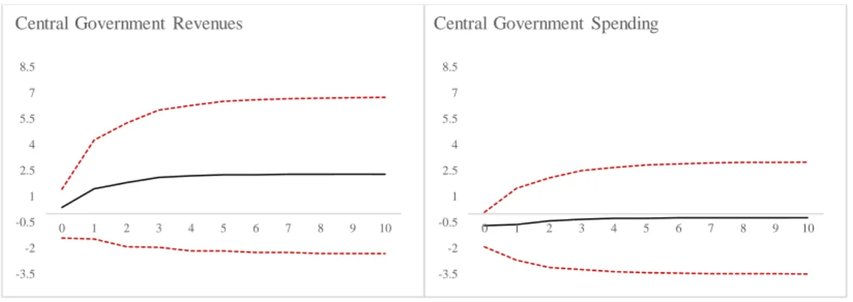
Figure 5 - Impulse Response of Fiscal Variables to One Standard Cholesky Innovation in Commodity Prices (In Percent)
Source: Author’s Elaboration -2 -1.5 -1 -0.5 0 0.5 1 1.5 2 2.5 3 3.5 0 1 2 3 4 5 6 7 8 9 10
Central Government Revenues
-2 -1.5 -1 -0.5 0 0.5 1 1.5 2 2.5 3 3.5 0 1 2 3 4 5 6 7 8 9 10
Figure 6 - Impulse Response of Fiscal Variables to One Standard Cholesky Innovation in Commodity Prices (In Percent)
Source: Author’s Elaboration
Figure 5 and 6 present the impulse response functions and the accumulated impulse response functions, respectively, of a one standard deviation commodity prices shock on central government revenues and central government spending, dotted and red lines indicates the 95% confidence error bands. Two interesting conclusions can be reached by the analysis of the graphs above. First, a shock to commodity price impacts government revenues by accelerating the its rate of growth about 1 % after one quarter of the shock, with the peak being at the 3 quarters after the shock. Second, a shock to commodity price seems not to affect government spending since its accumulated impact is nearly zero as showed in Figure 6. Moreover, I find a significant lower value for the impact on government expenditures than Medina (2010), who did this exercise for the first quarter of 1993 to the fourth quarter of 2008 and finds a positive accumulated impact of 2%. Note that for a great part of this time span, Brazil had not implemented the Fiscal Responsibility Law. I conjecture that the implementation of this fiscal rule in Brazil aided to reduce the volatility of the government expenditure to a shock to commodity prices.
I compute the forecasted error variance decomposition of commodity prices on government revenues and spending. The results are shown below.
-3.5 -2 -0.5 1 2.5 4 5.5 7 8.5 0 1 2 3 4 5 6 7 8 9 10
Central Government Revenues
-3.5 -2 -0.5 1 2.5 4 5.5 7 8.5 0 1 2 3 4 5 6 7 8 9 10
Table 5 - Variance Decomposition of Forecast Errors (In Percent) Quarter Government Revenues Government Spending 1 0.000 0.000 2 0.283 0.037 3 0.281 0.038 4 0.294 0.039 5 0.294 0.039 6 0.295 0.039 7 0.295 0.039 8 0.295 0.039 9 0.295 0.039 10 0.295 0.039
Source: Author’s Elaboration
The results show that the contribution of a shock to commodity prices is very low to the fluctuations on the government revenues, accounting for only 0.295% at a 10-quarter horizon during the period of analysis. In respect to the government spending this number is even lower with commodity price accounting for only 0.039%. As a conclusion, internal factors or other external factors are responsible to generate the majority of the fluctuations on the government revenues and expenditures.
The deterioration of Brazil fiscal balance might had been impacted by the cycle of commodity prices. The results of this sections suggest that the government revenues are cyclical with the commodity prices, while government spending (excluding social security expenses) is aligned only with the lag of the cyclical component of the commodity prices. After the 2008 crisis Brazilian government started to raise its expenditures until the beginning of the low phase of the commodity prices on 2015, however due to a limited ability to disinvest, the government was unable to adjust its expenditures to the new level of revenues. Thus, we can see the commodity prices shock as a trigger of the recent episode of fiscal crisis in Brazil.
5 Interest Rates
The literature has stressed that the borrowing costs of emerging countries is not only affected by internal factors but also by exogenous ones, such as risk appetite, contagious effects and commodities cycles. Fernandez et al. (2015) find that a rise on commodities prices have a strong negative effect on emerging market sovereign bonds. Shousha (2016) states that the negative correlation between commodity prices and interest rates is the major difference between emerging countries and developed commodities exporters. Furthermore, this relation had been explored in DSGE-models as being the main propagation channel of commodity prices shocks to the rest of the economy, such as in Shousha (2016), Dreschel and Tenreyro (2018), Farias (2017), and Fernandez (2018).
Indeed, if we look at the evolution of the country interest rate spread of Brazil alongside the real commodity prices index, as Figure 7 shows, we can see that Brazil real lending rate and commodity prices seem to follow an opposite path after 2001. When commodity prices raises, country interest rate spread declines. This fact could had been an important propagation mechanism of the commodity cycle for the Brazilian economy because, when the country spread reduces it can be a signal that the foreign investor sees Brazil as a safer country to invest.13
13 There is evidence that during the last commodity boom foreign direct investment rose in
Figure 7 - Interest Rates and Commodity Prices
Source: IMF, IBGE.Author’s Elaboration
Dreschell and Tenreyro (2018) and Rozada and Yeyati (2008) propose a simple way to understand how the commodity prices can affect emerging markets country spreads. First, suppose that there is a borrower who borrows the amount 𝐷𝑡. The probability she will repay in full is denoted by 𝑞, however with probability 1 – 𝑞, only the amount 𝜁, which is smaller than 𝐷𝑡, will be recovered. If we define 𝑟∗ as the risk free interest rate and 𝑟𝑡 as the interest rate of
this operation, the zero profit condition generated by neutral risk lender will be the following equation:
(1 + 𝑟∗)𝐷
𝑡 = 𝑞(1 + 𝑟𝑡)𝐷𝑡+ (1 − 𝑞)𝜁.
If we state that the amount to be recovered in case of default 𝜁, is equal to a proportion, 𝜃, of the commodity prices revenues, 𝑝𝑡𝑦𝑡, we get the following equation:
(1 + 𝑟∗)𝐷
𝑡 = 𝑞(1 + 𝑟𝑡)𝐷𝑡+ (1 − 𝑞)𝜃 𝑝𝑡𝑦𝑡,
thus, we get that the commodity prices and the interest rate spread is negative correlated with the commodity prices:
𝑟𝑡= 1 + 𝑟∗ 𝑞 − 1 − 𝑞 𝐷𝑡𝑞 𝜃 𝑝𝑡𝑦𝑡, 𝑟𝑡− 𝑟∗ = 1 − 𝑞 𝑞 (1 + 𝑟∗− 𝜃 𝑝𝑡𝑦𝑡). 0 0.05 0.1 0.15 0.2 0.25 0.3 0.35 0 20 40 60 80 100 120 140 1996Q1 1997Q1 1998Q1 1999Q1 2000Q1 2001Q1 2002Q1 2003Q1 2004Q1 2005Q1 2006Q1 2007Q1 2008Q1 2009Q1 2010Q1 2011Q1 2012Q1 2013Q1 2014Q1 2015Q1 2016Q1 2017Q1 Int er es t R ate C o m m o di ty P ric es
I explore these features through two different econometric analyses. The first one is based on the exercise made by Dreschell and Tenreyro (2018) for data from Argentina. The second one is based on Shousha (2016), but instead of running a panel-Var for a set of developing countries, I restrict the analysis to the estimation of a VAR for Brazil since it is the focus of this research.
5.1 Country Spreads and Commodity Prices Cyclicality
I estimate a set of regressions of Brazil real interest rate spread and the commodity prices index to shed further light on this topic. I define the regressions as follows:
𝑟𝑡− 𝑟𝑡∗ = 𝛼 + 𝜉 ln(𝑝
𝑡) + 𝛽𝑋𝑡+ 𝜖𝑡,
in which, 𝑟𝑡 is the real interest rate for Brazil, 𝑟𝑡∗ is a measure of world real interest rate, 𝑝𝑡 is the commodity prices index and 𝑋𝑡 is a vector of control variables including output growth, the debt to gdp ratio and the trade balance to gdp ratio. The parameter of interest here is 𝜉, which is the semi-elasticity of the interest rate spread to the commodity prices. In this analysis, I use the real lending rate as a measure of Brazil interest. I define the measure of the world interest rate in multiple ways, in one of them, I mimic Dreschell and Tenreyro (2018) by using the UK real interest rate offered by the Bank of England, so I can compare their result for Argentina with mine for Brazil. Alternatively, I use the real lending rate of United States, so the country interest rate spread would reflect the difference of costs of a similar operation in Brazil and in United States. I estimate the model with annual data from 1997 to 2017.14
14 Other estimations are made using different measures of country interest rate spread and they
Table 6 - Real Spread Regressions (using UK interest rate) Dependent Variable (1) (2) (3) (4) (5) Real Spread Constant 0.734*** 0.732*** 0.786*** 1.007*** 0.867*** (0.0664) (0.0685) (0.072) (0.213) (0.289) Commodity Prices -0.0037*** -0.0037*** -0.0044*** -0.0047*** -0.0048*** (0.0008) (0.0008) (0.0009) (0.0011) (0.0011) Output Growth 0.169 0.477 (0.8274) (0.837) Trade Balance to GDP -1.496 -1.294 (0.962) (1.548) Debt to GDP -0.473 -0.161 (0.351) (0.551) Observations 21 21 21 21 21 R Square 0.497 0.498 0.556 0.543 0.567 F-Statistic 18.78*** 8.94*** 11.3*** 10.7*** 5.25*** Signif. Codes: 0.01*** 0.05** 0.1*
Source: Author’s Elaboration
Table 7 - Real Spread Regressions (using US interest rate)
Dependent
Variable (1) (2) (3) (4) (5)
Real Rate Spread
Constant 0.722*** 0.719*** 0.768*** 0.990*** 0.8933*** (0.0642) (0.0662) (0.0706) (0.2061) (0.2804) Commodity Prices -0.0039*** -0.0040*** -0.0046*** -0.0049*** -0.0050*** (0.00083) (0.00086) (0.00093) (0.00108) (0.00116) Output Growth 0.2684 0.550 (0.7987) (0.8121) Trade Balance to GDP -1.327 -0.9674 (0.9407) (1.5019) Debt to GDP -0.463 -0.2467 (0.3395) (0.5351) Observations 21 21 21 21 21 R Square 0.546 0.548 0.591 0.5886 0.607 F-Statistic 22.85*** 10.95*** 13.02*** 12.88*** 6.189*** Signif. Codes: 0.01*** 0.05** 0.1*
Table 6 and 7 show the estimations of the regressions by ordinary least square. It is interesting to note that the results of the two specifications for the country spreads do not change drastically. The sign of the coefficient associated with commodity prices is statistically significant and negative in all specifications. When we control for other variables, such as trade balance and output growth, the results are still robust. This result suggests that a rise on commodity prices allows the difference between Brazil interest rate and the international interest rate to narrow, thus allowing Brazil to be perceived as a safer country to invest internationally. Specifically, if we consider the lowest value of 𝜉, a rise in 1% of the real commodity prices index reduces the country spread by 0.37%. This coefficient is significantly lower than the one Dreschell and Tenreyro (2018) find for Argentina. They find that the same impact for Argentina allowed the country spread to reduce by 2%. Thus, comparing these two countries, Brazil tends to have a lower vulnerability to the commodity prices effect on the interest rates.
5.2 Country Spreads and Commodity Prices Shocks
In this subsection, I evaluate the impact of a shock to commodity prices on not only the country interest rate spread but also on other domestic variables. I estimate the VAR based on Shousha (2016): 𝑦𝑡 = ∑ 𝐴𝑗𝑦𝑡−𝑗 𝐽 𝑗=1 + 𝑢𝑡 𝑦𝑡 = [𝑝𝑡, 𝑟𝑡∗− 𝑟 𝑡, 𝑔𝑑𝑝𝑡, 𝑡𝑏𝑡, 𝑐𝑟𝑡, 𝑟𝑡, 𝑟𝑒𝑒𝑟𝑡],
in which 𝑝𝑡 is the real commodity prices index, 𝑟𝑡∗− 𝑟
𝑡 is the Brazil interest rate spread to US,
𝑔𝑑𝑝𝑡 is Brazil real gross domestic product, 𝑡𝑏𝑡 is the real trade balance to gdp, 𝑐𝑟𝑡 is the credit
to the non-financial sector, and 𝑟𝑒𝑒𝑟𝑡 is the real exchange rate. All variables are in difference of their logs, with exception of the trade balance and the lending rates that are computed in level differences. The variables are in quarterly frequency and deseasonalized. The data starts in the first quarter of 1997 and goes to the fourth quarter of 2017. The number of included lags (𝐽) was defined using the Schwarz Criterion.
I compute the structural parameters of the model by the orthogonalization of the structural errors through a Cholesky decomposition. I order commodity prices first assuming that Brazilian economy is small enough to not affect commodity prices. I order country spread second since the literature stresses the country spread as one of the main transmission channel
of a shock to commodity prices. I assume that the output lead the cycle of the domestic variables, therefore, the remaining variables are ordered as, output, credit to the non-financial sector, trade balance, and exchange rate.15
First, I compute the impulse response function of one standard deviation commodity prices shocks, which means a 3% increase on the real commodity index, and the accumulated impulse response functions.
Figure 8 - Impulse Response Function to a one standard deviation shock in commodity prices
Source: Author’s Elaboration
15Relaxing those assumptions does not change the main results. -0.02 0 0.02 0.04 0.06 0.08 0.1 0.12 5 10 15 Commodity Prices -0.015 -0.01 -0.005 0 0.005 0.01 5 10 15 Country Spread -0.002 0 0.002 0.004 0.006 0.008 0.01 5 10 15 Output -0.004 -0.003 -0.002 -0.001 0 0.001 5 10 15 Trade Balance -0.015 -0.01 -0.005 0 0.005 0.01 0.015 5 10 15 Real Credit -0.07 -0.06 -0.05 -0.04 -0.03 -0.02 -0.01 0 0.01 0.02 5 10 15 Exchange Rate
Figure 9 - Accumulated Impulse Response Function to a one standard deviation shock in commodity prices
Source: Author’s Elaboration
The Figures 8 and 9 plot the impulse response functions and the accumulated impulse response functions, dotted red lines indicate the 95% confidence error band. Some results are aligned with the literature. This model stresses the negative correlation between commodity prices and Brazil country spread. A commodity prices shock allows the interest rate spread to reduce about 0.4% right in the moment of the shock. The output also accelerates in the moment of the shock, confirming the importance of this shock to the Brazilian economy. The real credit to the non-financial sector does not respond immediately, it starts to respond to the commodity shock 2 quarters after the shock, however on the long term the impact is economically significant, increasing 0.7% the credit inside the Brazilian economy.
Shousha (2016) finds that the commodity prices depreciate the exchange rate and improves the trade balance position for developing economies. This is quite different from my result for Brazil, the commodity prices shocks appreciate the exchange rate and deteriorate the trade balance in this model. An explanation for that is related to the capital inflows to Brazil during the last commodity boom. This allowed the exchange rate to appreciates, and, since the domestic economic activity have grown, it allowed the country to import more, nullifying the extra revenues from the commodity exports.
0 0.05 0.1 0.15 0.2 0.25 0.3 5 10 15 Commodity Prices -0.04 -0.03 -0.02 -0.01 0 0.01 0.02 5 10 15 Country Spread -0.005 0 0.005 0.01 0.015 0.02 0.025 0.03 0.035 5 10 15 Output -0.01 -0.008 -0.006 -0.004 -0.002 0 0.002 0.004 5 10 15 Trade Balance -0.03 -0.02 -0.01 0 0.01 0.02 0.03 0.04 0.05 5 10 15 Real Credit -0.12 -0.1 -0.08 -0.06 -0.04 -0.02 0 0.02 5 10 15 Exchange Rate
To understand the contribution of this shock for the different variables, I perform the variance decomposition of the forecast errors. Table 8 shows the results. The commodity prices shock is more important to the real output and to exchange rate. Shousha finds that the commodity prices contribute to 23% to the output variance, while I found it to be 26% for Brazil. This number suggests that 26% of the 2016 crisis was impacted by the fall of the commodity prices on that period. The low contribution to the country spread might be related to the fact that domestic interest rate and US interest rate are affected by internal and external factors that goes beyond the model.
Table 8 - Variance Decomposition of Forecast Errors
Quarter 5 10 15 20 Country Spread 0.0315 0.0316 0.0316 0.0316 Output 0.2783 0.2696 0.2686 0.2684 Trade Balance 0.0284 0.0284 0.0285 0.0284 Real Credit 0.0332 0.0413 0.0436 0.0437 Exchange Rate 0.1007 0.1155 0.1156 0.1156
6 Sectorial Impacts
In this section, I analyze how the sectors of Brazilian economy are affected by the commodity prices shocks. To do so, I divide the Brazilian economy in three sectors, first, the commodity sectors, which is composed by the Agricultural sector and Extractive Industry sector. Second, I define the general industry sector, composed by the Electricity and Gas, Water, Sewage and Waste Management Activities sector, the Transformation Industry sector and the Construction sector, and third, the Service Sector. The commodity prices can affect these sectors in multiple ways along their value chain. For example, it is intuitive to think that a rise on the commodity prices might augment the production value of the commodity sector, which, in turn, will acquire more products from the service sector and more machineries from the general industrial sector, this is the result Knop and Vespignani (2014) find for the Australian economy. However, one might think that the rise on the commodity prices might augment the prices of food and fuel which rises the costs of the industrial and the services sectors, and, thus decreasing its output, just like Fukunaga et al. (2010) find for US and Japan industries.
Figure 10 - Sectorial Added Values (R$ Millions)16
Source: IBGE, Author’s Elaboration.
16 1995 prices 0 200000 400000 600000 800000 1000000 1200000 1996 1998 2000 2002 2004 2006 2008 2010 2012 2014 2016 Commoditty Industry Service
Figure 11 - Share on Aggregated Added Value
Source: IBGE. Author’s Elaboration
Figure 13 shows the real added value of these three sectors in the last 20 years, while Figure 14 shows the participation of each sector on the aggregate added value for selected years. As can be seen, the commodity sector is the smallest from the three. While services sectors account for 70% of the aggregate value added, general industry accounts for 21% and the commodities sector represents only 9% in 2017. Even though the commodity sector is only a small part of the value added, this sector was the fastest growing from 1997 to 2017, augmenting 117%, while the general industry sector and the services sector grew 29 % and 66% on this period, respectively. 0.0% 10.0% 20.0% 30.0% 40.0% 50.0% 60.0% 70.0% 80.0% 1997 2002 2007 2012 2017
Figure 12 - Commodity exports (% as share of total exports)
Source: UN Commtrade. Author’s Elaboration
Additionally, commodity products are a significant part of the Brazilian exports. Figure 12 shows the evolution of the share of commodity exports from Brazil. I define as commodity product the primary fuels and lubricants exports, the primary food and beverage exports, and the primary industrial supplies, all according to the Broad Economic Categories classification from the Standard International Trade Classification. The graph shows that Brazil commodity exports dependence grew in the last decade. In the beginning of century commodity exports represented only 16%, however with the rise tendency of the commodity prices beginning on 2003, its importance grew to 40 % in 2011.
In order to study the impacts that the commodity prices shocks had on those sectors of the Brazilian economy, the following subsection analyzes this issue empirically through the estimation of a VAR.
6.1 Commodity Prices shock on Brazilian Sectors
I base the following VAR model on Bergholf et al. (2017), they run a simple VAR for the Norwegian economy to evaluate the impacts of a shock to oil prices on different sectors of the economy. I adapt their model to analyze the impact of commodity prices shocks on the three sectors of the Brazilian economy, as defined previously. Formally, I estimate:
𝑦𝑡 = ∑ 𝐴𝑗𝑦𝑡−𝑗 𝐽 𝑗=1 + 𝑢𝑡, 0 5 10 15 20 25 30 35 40 45
𝑦𝑡 = [𝑦̃𝑊,𝑡, 𝑝𝑐,𝑡, 𝑒𝑡, 𝑦̃𝑐, 𝑦̃𝑠, 𝑦̃𝑚] , 𝑢𝑡 ~𝑖𝑖𝑑𝑁(0, 𝛴).
The model consists of quarterly data on two international variables, 𝑦̃𝑊,𝑡, the real world gdp, consisting of the sum of the real gross domestic product (GDP) in US dollars of China, Euro Area and United States, and the commodity prices, 𝑝𝑐,𝑡. The domestic variables are the
real exchange rate of Reais per US Dollar, 𝑒𝑡, added value in the sector of commodities, 𝑦̃𝑐,
services, 𝑦̃𝑠 and manufacturing, 𝑦̃𝑚. In order to deal with unit root issues, I run the model transforming every variable in their difference of log. The VAR is run with data form the first quarter of 1996 to the fourth quarter of 2017 and the number of lags is defined by the Schwarz Criterion.
Since there are two international variables, I decided to impose a Cholesky decomposition of the error in order to identify the structural parameters of the model and to compute the impulse response functions. The block of foreign variables was ordered first, in the sense that Brazil is a small economy and it is incapable of affecting those variables contemporaneously. The global gdp was ordered first and the commodity prices second, thus global gdp can affect contemporaneously the commodity prices in this model. As the main focus is to analyze the impact of a commodity prices shocks on Brazilian economy sectors, I decide not to identify the shocks from the domestic variables. In order to compare the effects of a global shock and commodity prices, I offer the impulse response function of both variables below.
Figure 13 - Impulse Response Function to a one standard deviation shock in commodity prices (sectorial analysis)
Source: Author’s Elaboration -0.08 -0.06 -0.04 -0.02 0 0.02 0 5 10 Exchange Rate -0.01 -0.005 0 0.005 0.01 0.015 0 5 10 Commodity Sector -0.01 -0.005 0 0.005 0.01 0.015 0.02 1 6 11 Industry Sector -0.002 0 0.002 0.004 0.006 0.008 1 6 11 Service Sector
Figure 14 - Accumulated Impulse Response Function to a one standard deviation shock in commodity prices (sectorial analysis)
Source: Author’s Elaboration
Figure 13 and Figure 14 present the impulse response functions and the accumulated impulse response functions of a one standard deviation shock to commodity prices on the domestic variables, 95% confidence interval error bands are provided by the red and dotted lines. The impact of the shocks on the domestic variables is economically significant, and it lasts at most 6 quarters. A standard deviation shock on the commodity prices represents a positive 6% increase on the commodity prices index. The exchange rate has the quickest, but strongest effect, right in the period of the shock it appreciates 0.4%, with its peak being at the third quarter after the shock. This result is aligned with the results from section 5.
The commodity prices do not impact negatively the industrial sector. A possible explanation is that the commodity prices shock rather than dislocating the resources from the industrial sector, it complements this sector, probably by trading inside the Brazilian economy. However, we must keep in mind that further investigation is needed to validate this argument. Additionally, the strongest effect is not on the commodity sector but on the industrial sector, which is probably explained by the size of those sectors. Bergholf at al. (2017), find similar results for Norway. In their model, a rise on the oil prices does not crowd out resources from the manufacturing sector.
-0.16 -0.14 -0.12 -0.1 -0.08 -0.06 -0.04 -0.02 0 0 5 10 Exchange Rate -0.02 -0.01 0 0.01 0.02 0.03 0.04 0 5 10 Commodity Sector -0.01 0 0.01 0.02 0.03 0.04 0.05 0 5 10 Industry Sector -0.005 0 0.005 0.01 0.015 0.02 0.025 0 5 10 Service Sector
Figure 15 - Impulse Response Function to a one standard deviation shock from world GDP
Source: Author’s Elaboration
Figure 16 - Accumulated Impulse Response Function to a one standard deviation shock from world GDP
Source: Author’s Elaboration.
Figure 15 and 16 present the impulse response functions and the accumulated impulse response functions of a one standard deviation global shock. Starting with the exchange rate, we see that the effects of a global shock also causes an appreciation of this variable, moreover, the effect is similar to the commodity prices shock on numbers, however, this one last shorter. Looking at the domestic variables, we see that all the domestic sectors respond positively to a positive world shock and its effect last for about one year, which is consistent with the fact that Brazil is an open small economy. The service sector is the most affected by the world shock, followed by the industrial sector and the last is the commodity sector.
-0.02 -0.015 -0.01 -0.005 0 0.005 0.01 0.015 0 5 10 Exchange Rate -0.015 -0.01 -0.005 0 0.005 0.01 0.015 0 5 10 Commodity Sector -0.006 -0.004 -0.002 0 0.002 0.004 0.006 0.008 0 5 10 Industry Sector -0.002 -0.001 0 0.001 0.002 0.003 0.004 0 5 10 Service Sector -0.06 -0.04 -0.02 0 0.02 0.04 0 5 10 Exchange Rate -0.03 -0.02 -0.01 0 0.01 0.02 0.03 0 5 10 Commodity Sector -0.015 -0.01 -0.005 0 0.005 0.01 0.015 0.02 0.025 0 5 10 Industry Sector -0.004 -0.002 0 0.002 0.004 0.006 0.008 0.01 0 5 10 Service Sector
Table 9 - Forecast Error Variance Decomposition from Commodity Prices (Sectorial Analysis) Quarter Exchange Rate Commodity Sector Industry Sector Service Sector 1 0.0019 0.0019 0.0068 0.0057 2 0.0024 0.0032 0.0081 0.0146 3 0.0025 0.0033 0.0083 0.0179 4 0.0025 0.0035 0.0085 0.0192 5 0.0025 0.0035 0.0085 0.0196 6 0.0025 0.0035 0.0085 0.0198 7 0.0025 0.0035 0.0085 0.0198 8 0.0025 0.0035 0.0085 0.0198 9 0.0025 0.0035 0.0085 0.0198 10 0.0025 0.0035 0.0085 0.0198
Source: Author’s Elaboration
Table 10 - Forecast Error Variance Decomposition from Real World GDP (Sectorial Analysis)
Quarter
Exchange Rate
Commodity
Sector Industry Sector
Service Sector 1 0.0007 0.0157 0.0299 0.0337 2 0.0007 0.0170 0.0332 0.0350 3 0.0007 0.0183 0.0352 0.0359 4 0.0007 0.0183 0.0353 0.0362 5 0.0007 0.0184 0.0353 0.0362 6 0.0007 0.0184 0.0353 0.0363 7 0.0007 0.0184 0.0353 0.0363 8 0.0007 0.0184 0.0353 0.0363 9 0.0007 0.0184 0.0353 0.0363 10 0.0007 0.0184 0.0353 0.0363
Source: Author’s Elaboration
The contribution of the commodities prices and the real world GDP to the forecast error variance decomposition of the domestic variables is offered by the Table 10 and Table 11, respectively. The results from this model is quite different from the one in section 4. Here, the contributions of the commodities prices to the added value on the domestic variables only surpass 1 % on the service sector. This result is quite puzzling, since we find that the contribution of this variable is 26% to Brazil output on the other model. Probably, this contribution is lost when we divide Brazil output in sectorial added value and the interconnections between those sectors during a commodity prices shocks decrease its
influence. The contribution of the world real gdp shock is significantly larger than the commodity prices’ one to Brazilian added values sectors. The contribution of this variable to the industry and commodity sectors are almost equal, about 3.5 %. It is interesting to note that the contribution to the exchange rate is much lower than the one from commodity prices.
In sum, three interesting conclusions can be derived from the graphs above, first commodity prices and world demand, in the way they are defined here, generate spillover to Brazil economy. Second the commodity prices shocks, do not crowds out the industry sector, on the contrary, it causes spillovers to this sector. Lastly the contribution of world shocks to the variance of the forecast errors of Brazilian domestic variables is stronger than the one from the commodity prices.