Célio Duarte Pereira Oliveira
UMinho|20
14
abril de 2014
Education and Labour Mark
et T
ransitions: A Sur
vival Analysis Using P
or
tuguese Dat
a
Universidade do Minho
Escola de Economia e Gestão
Education and Labour Market Transitions:
A Survival Analysis Using Portuguese Data
Célio Duar
te P
er
Dissertação de Mestrado
Mestrado em Economia
Trabalho realizado sob a orientação do
Professor Doutor João Cerejeira
e da
Professora Doutora Carla Sá
Célio Duarte Pereira Oliveira
abril de 2014
Universidade do Minho
Escola de Economia e Gestão
Education and Labour Market Transitions:
A Survival Analysis Using Portuguese Data
ii
Declaração
Nome: Célio Duarte Pereira Oliveira
Endereço Electrónico: [email protected]
Título da Dissertação:
Education and Labour Market Transitions: A Survival Analysis Using Portuguese Data
Orientadores:
Professor Doutor João Cerejeira Professora Doutora Carla Sá
Ano de Conclusão: 2014
Designação do Mestrado: Mestrado em Economia
É AUTORIZADA A REPRODUÇÃO INTEGRAL DESTA DISSERTAÇÃO APENAS PARA EFEITOS DE INVESTIGAÇÃO, MEDIANTE DECLARAÇÃO ESCRITA DO INTERESSADO, QUE A TAL SE COM-PROMETE;
Universidade do Minho, ___/___/______
iii
Acknowledgments
I would like to give a special thanks to my supervisors, Doctors João Cerejeira and Carla Sá, for their continuous guidance and pertinent commentaries during the past year. This work benefitted from their advice, especially from the meticulous corrections of Dr Carla Sá, the enlightening comments Dr João Cerejeira, and their sense of humour in our meetings.
I would also like to Doctor Miguel Portela for all his patience, and energy, for all my questions and doubts during our walks to the coffee machine, an always good counsellor.
To my parents, my sister and all my friends, whose names I will not mention, for their continuous support, thank you! Without them my life would be empty of joy and meaningless.
v
Education and Labour Market Transitions: A Survival Analysis Using
Portuguese Data
Abstract
In the recent past, there has been a generalized investment in education across several countries including Portugal; however the rising of educational driven by youths has been followed by an increase in unemployment rate, with especial incidence among youths.
Using a duration analysis framework in continuous time and the Portuguese LFS from 1998 to 2009, we aim to evaluate the role of education in labour market. Namely, we want to access whether education prevents unemployment for those who have a job and whether if it helps un-employed finding a job.
Our results show that more educated individuals, with a high school diploma or higher, have low-er hazard of job loss. Among those who lost their job or are looking for their first job, we found evidence that college graduates have higher prospects of finding a job. Those results seem to suggest that employers prefer more skilled workers, in accordance with the idea that education increases the individual’s productivity.
vii
Educação e Transições no Mercado de Trabalho: uma análise de
sobrevivência usando dados nacionais.
Resumo
No passado recente, tem havido um aumento generalizado da educação em vários países, inclu-indo Portugal. Contudo o aumento do nível educacional da população fomentado pelos mais no-vos tem sido acompanhado por um aumento das taxas de desemprego, com maior incidência sobre os mais jovens.
Usando modelos de duração em tempo contínuo com dados Portugueses do LFS de 1998 até 2009 tentamos avaliar o papel da educação no mercado de trabalho. Nomeadamente, avaliar se a educação previne o desemprego entre aqueles que estão a trabalhar e se ajuda os desempre-gados a encontrar emprego.
Os nossos resultados mostram que os indivíduos com maior nível de educação, com ensino se-cundário ou superior, têm menor probabilidade de perder o emprego. Entre aqueles que não têm emprego ou estão à procura do primeiro emprego, encontramos evidência que o ensino superior aumenta a possibilidade de encontrar emprego. Estes resultados parecem sugerir uma maior preferência dos empregados por indivíduos com maior formação, em concordância com a ideia de que a educação aumenta a produtividade dos indivíduos.
Palavras-chave: educação, transições no mercado de trabalho, emprego, desemprego,
ix
Contents
1 Introduction ________________________________________________________ 1 2 Theoretical background _______________________________________________ 3 3 Duration Analysis ____________________________________________________ 9 3.1 Single Risks ____________________________________________________ 9 3.2 Competing Risks ________________________________________________ 123.3 Stratified Proportional Hazard Model __________________________________ 14
4 Data and model specification ___________________________________________ 15
4.1 The data ______________________________________________________ 15
4.2 Model Specification ______________________________________________ 18
4.2.1 From employment to unemployment ________________________________ 18
4.2.2 From unemployment to employment ________________________________ 21
5 Results and discussion _______________________________________________ 25
5.1 From employment to unemployment _________________________________ 25
5.2 From unemployment to employment _________________________________ 29
5.3 Discussion____________________________________________________ 36 6 Conclusion _______________________________________________________ 39 7 References ________________________________________________________ 41 Appendix _____________________________________________________________ 45 Data preparation _________________________________________________ 45 A.
Stratified models by economic activity ___________________________________ 47 B.
Cumulative Incidence Functions (competing risks) _________________________ 48 C.
Baseline Hazard Function Plot ________________________________________ 52 D.
x
List of Tables
Table 1 – Descriptive statistics and variable definition: From employment to unemployment __ 20 Table 2 – Descriptive statistics and variable definition: From unemployment to employment __ 22 Table 3 – Cause-specific hazard of unemployment estimation results __________________ 26 Table 4 – Cause-specific hazard of employment estimation results ____________________ 30 Table 5 – Outliers conditions based on age, from authors __________________________ 45 Table 6 – Outliers conditions based on Education, from authors _____________________ 45 Table 7 – Outliers condition based on job's occupation description, from authors _________ 46 Table 8 – Sectors of Economic Activity. ________________________________________ 47 Table 9 – Cumulative Incidence Function of Unemployment ________________________ 48 Table 10 – Cumulative Incidence Function of Employment__________________________ 50
List of Figures
Figure 1 – Estimated baseline hazard curve of unemployment from Cox model (model 7) ___ 53 Figure 2 – Estimated baseline hazard curve of employment from Cox model (model 4) ______54
xi
List of abbreviations and acronyms
CIF: Cumulative Incidence Function EU: European Union
IE: Inquérito ao Emprego (Labour Force Survey)
INE: Instituto Nacional de Estatística (Statistics Portugal)
LFS: Labour Force Survey LIFO: Last In First Out LR: Long-run
NUTS: Nomenclatura de Unidades Territoriais para fins Estatísticos (Nomenclature of Territorial Units for Statistics)
OECD: Organisation for Economic Co-operation and Development PCE: Piecewise-Constant Exponential
PH: Proportional Hazard
PSID: Panel Study of Income Dynamics SR: Short-run
1
1
Introduction
In the recent past, there has been a generalized investment in education across several countries
including Portugal (OECD, 2009)1. The investment in education is guided by the belief that
educa-tion has positive effects for the individual as well as for the society.
At the individual level, the higher the human capital the higher the potential wage. By investing in education an individual is increasing her human capital and therefore her potential wage in the labour market (Psacharopoulos and Patrinos, 2004). Other individual benefits include lower chances of becoming unemployed, and lower unemployment durations in the event of unem-ployment. Education is expected to ease transitions in the labour market, and the fact that it
im-proves individual’s adaptability to changes2 is among the possible explanations. The more
edu-cated the individual, the higher the opportunity cost of being unemployed or out of labour market (inactive).
The social benefits of education have been broadly study. Several studies highlight the positive impact of education on productivity (Moretti, 2004b), and the causal impact of education on countries’ economic growth, especially the quality of education (Barro, 2000; Hanushek and Wößmann, 2007). Additionally, higher levels of education may lead to higher levels of wealth, it may lower the probability that individuals engage in activities that generate negative externalities (such as crime), as well as it may improve the quality of elections and, consequently, the quality of the democracy (Moretti, 2005).
In the current economic context of anaemic growth in combination with higher educational levels and increasing unemployment rates (particularly among the youngsters) makes the study of cation and labour market transitions more relevant. A better understanding of the impact of edu-cation on the employment-unemployment flows may be useful in designing more effective job policies addressing the labour market participation of the new qualified workers.
1 For the OECD countries the education expenditure per student was 24% higher in 2006 than 2000 for non-tertiary level, and
11% higher for tertiary level. Portugal, also registered an increase of 12% and 35% for non-tertiary and tertiary levels, respectively.
2 The Pedagogy for Employability Group (2012) point many attributes valued by the employers, many of them can be related to
2
The aim of this research is to evaluate how education affects the labour market transitions, name-ly to check whether more educated individuals have lower risk of job loss (transition from em-ployment to unemem-ployment), and once unemployed, whether it increases the chance of re-em-ployment (transition from unemre-em-ployment to emre-em-ployment).
The empirical analysis uses data from the Portuguese Labour Force Survey, for the period be-tween 1998 and 2009 (second quarter). The dataset is build based on quarterly data allows for the application of survival analysis techniques. Two models are estimated to analyse the role of education on both, the transition from employment to unemployment and the re-employment probability of the unemployed workers, respectively.
The main contributions of this research relate to its empirical approach. First, we use a panel da-taset, which covers a long period of time. Second, we use continuous time survival models, ra-ther than discrete time models as used before. Third, two transitions are analysed, namely from employment to unemployment and from unemployment to employment, which allows for a better understanding of the role of education on labour market transitions.
The remaining of this research is structured as follows. Section 2 discusses the theoretical back-ground and the main results of previous studies. Section 3 introduces the methodology to be used. Section 4 presents the data and empirical model, and Section 5 discusses the estimation results. Finally, Section 6 closes with the main conclusions, the discussion of some limitations of the analysis, and pointing some ways for further work on the topic.
3
2
Theoretical background
The relationship between labour market outcomes and education has long been of interest for economists. For instance, Mincer (1991) evaluated the impact of education on the unemployment rate for USA, using the PSID (Panel Study of Income Dynamics) dataset from 1976 to 1983. The results showed that the higher the education level, the lower the unemployment rate, the easier to move to another job, and the higher the stability of the current job (measured in terms of its dura-tion).
The individuals take the decision to invest in education (human capital) if they expect its benefits to outweigh the costs, that is, if they expect positive net returns. The existence of positive returns on education is an indicator that education may increase the individuals’ productivity, an attribute valued by employers. (See Psacharopoulos, 1985; Psacharopoulos and Patrinos, 2004; Weiss, 1995; and Chevalier, Harmon, Walker and Zhu, 2004).
The benefits that an investment in education brings are not restricted to private returns; we shall consider the existence of social returns as well. From the government point of view, the decision to invest in education is based on the existence of social gains. Moretti (2004a) studied the exist-ence of non-private returns in the US when there is an increase of the labour force share of col-lege graduates within a city. He found a positive spillover effect of colcol-lege graduates, by compar-ing similar individuals who work in cities with different shares of college graduates in the labour force. After controlling for unobserved characteristics of the individuals and the cities, he con-cludes that 1% increase in the proportion of college graduate workers raises the wages of high school dropout workers by 1,9%, of the high school graduates by 1,6% and of the college gradu-ates by 0,4%. The wage increase resulting from an increase in the proportion of college gradugradu-ates workers is larger for less educated workers as predicted by a demand and supply model.
According to the screening and signalling theories, the educational level observed by the ployer reduces the information asymmetry about the unobserved productivity of the potential em-ployee. The more productive individuals invest in education in order to signal their higher produc-tivity and by doing so get a better salary (see Spence, 1973; Stiglitz, 1975; Layard and
4
Psacharopoulos, 1974; and Weiss, 1995). The crowding-out3 theory presents itself as an
explana-tion for the lower unemployment rates among the more educated (skilled) workers. Employers have preferences on the abilities of their employees, and the actual and potential workers are ranked accordingly. Therefore, the human capital theory and the screening theory suggest that, on average, the more educated/skilled ones are ranked above the less educated/skilled, being the first, which explain the lower unemployment rate among the former.
Education also may explain the lower unemployment rate by affecting the type of job search methods as well as the searching intensity. In an evaluation for several European countries using European Union Labour Force Survey (EU-LFS) from 2006 to 2008, Bachmann and Baumgarten (2012) apply a ordered logit and a probit model to find out the determinants of job search meth-ods among unemployed workers. They concluded that the more educated and the younger
work-ers search with more intensity4. In general, unemployed women search less intensely than man,
and family characteristics such as the number of children and the number of elderly living in the household are associated with lower levels of search intensity. They also found the existence of heterogeneity of job search methods among countries. In Mediterranean countries like Spain, Italy and Greece informal search methods are preferred over the public employment office; whereas in the Central and Eastern European countries the workers prefer the direct methods over the public employment office.
Addison and Portugal (2002) use data from the Portuguese LFS (Inquérito ao Emprego) in the 1990s to estimate the effectiveness of job search methods to escape from unemployment. The authors found that search for a job using the public employment service leads to jobs that last and pay less than jobs obtained via other search methods. They also expected to see individuals selecting the job search methods that give them the best chances of finding a new job. The use of direct search methods and informal networks is the most preferred (which contrasts with the results found in the British literature), however, it does assures better chances of finding a job but it is not associated to higher earnings.
Núñez and Livanos (2009) used a multinomial-logit model to access the impact of the education level and the field of study in the short and long run unemployment applied to the EU-15 based
3 For more details about the crowding-out theory and the job competition model, see Teulings and Koopmanschap (1989), and
Thurow (1975), respectively, cited by Wolbers (2000).
5
on EU-LFS micro-data for the spring quarter of 2005. Both the education level and the field of study are shown to have an effect on the transitions from short-run (SR) unemployment to em-ployment and from SR unemem-ployment to long-run (LR) unemem-ployment. In general, the results suggest that higher education is associated to better chances of finding a job; as well as a more modest effect preventing the LR unemployment. When the effect of getting a higher education diploma is compared among countries, the results are heterogeneous. College graduates in coun-tries like Finland, Belgium and the UK has the strongest positive effect of employment (condition-al on being a SR unemployed worker). Conversely, college graduates in countries like Portug(condition-al, Italy, and Greece face the lowest likelihood of finding a job (when compared to college graduates in other countries), which may be a signal of labour market problems. Regarding the field of study, the results show unequal employment opportunities across different fields5. The fields more successful preventing the SR unemployment are education, engineering, health and wel-fare, and services and tourism, whereas sciences, biology and environment, computer use, and health and welfare appear to be more effective preventing the LR unemployment.
Riddell and Song (2011a, b) intended to evaluate the relation between education and the labour market using instrumental variables. In Riddell and Song (2011b), the authors studied the exist-ence of a causal effect of education on the probability of re-employment conditional on being un-employed one year earlier. This study was motivated by the idea that more educated and/or
skilled individuals make wiser decisions when the status quo changes. To test their assumption
they used the US Current Population Data (1980-2005) and the 1980 Census. In order to ad-dress the education endogeneity problem, they used changes in the compulsory schooling laws and children labour laws as instrumental variables to school graduation. To instrument
high-er education they also used the conscription risk in the Vietnam War6. In general, the higher the
educational level the higher the chances of re-employment. They found positive non-linear results, with higher effects around 12 and 16 years of schooling, suggesting the presence of sheepskin effect. Regarding the effect of education in unemployment incidence the results show that college graduation is associated to lower prevalence of unemployment, but no causal relationship at the high school was found.
5 The reference category is social business and law.
6
The same approach has been implemented using Canadian data such as the LFS (1976-1996), and the Census (1981, 1986, 1991, 1996 and 2001) Public Use Microdata Files. In this case, Riddell and Song (2011a) used changes in the compulsory schooling laws over time and across jurisdictions as instrumental variables for education. Besides the analysis performed to the US presented before, the authors also studied the effect of education on job search intensity. They found evidence that education measured by a dummy for high school graduation or years of schooling has a positive causal effect on job search intensity. Regarding employment, the sults are in line with the results found with the US data, namely schooling enhances the re-employment chances.
The risk of unemployment can be view under two perspectives: first, there is the risk of job loss, and, second, once unemployed there is a risk of not finding a job. Lauer (2003) analysed both risks in a comparative study for France (Emploi survey) and Germany (German Socio-Economic Panel – GSOEP) in the 1990s. The author used a discrete time framework with competing risks hazard rate model with a semi-parametric specification of the baseline hazard function (piecewise constant). He proposes a competing risks model under a discrete time framework using multi-nomial-logit estimation. In general, the results for both countries show that education lowers the risk of unemployment; the individuals with the lowest level of education and no vocational educa-tion have the highest risk of unemployment. Ceteris paribus, finishing higher educaeduca-tion appears to be more effective protecting individuals from unemployment in France, whereas, in Germany, getting vocational qualification (intermediate level) ensures more protection against unemploy-ment. A common characteristic to both countries is that individuals holding lower tertiary educa-tion qualificaeduca-tions show lower risk of job loss than those who have upper tertiary qualificaeduca-tions. A possible explanation may be that lower tertiary degrees are more practical and more oriented to the economy’s demand. Education also plays a role by increasing the possibilities of leaving un-employment and finding a job. Higher education graduates show higher probability of re-employment, with a small difference on the re-employment probability between workers with the lower tertiary level and the upper tertiary levels.
Summarizing, in France the risk of job loss is higher7 than in Germany, for every educational level,
as are the re-employment prospects. So, the German workers face a lower risk of unemployment,
7 The unemployment rate is higher in France than in German, particularly for individuals with basic vocational and intermediate
7
but if unemployed it is harder for them to find a new job. In Germany, holding a vocational qualifi-cation (intermediate level) is the best insurance against unemployment, but it is the higher educa-tion diploma that enhances the chance of re-employment. In France, the higher educaeduca-tion degree is associated with a lower risk of unemployment and a higher probability of exiting from unem-ployment. These results may explain the higher demand for vocational qualifications in Germany, whereas in France people invest more in higher education qualifications.
Wolbers (2000) intended to understand and test whether less educated workers have higher chances of job loss and experience longer unemployment duration than more educated individu-als, as well as to evaluate whether such phenomenon is stronger during recession periods of the labour market. In other words, the author aimed to access the impact of educational level on la-bour market transitions and if this relation is affected during lala-bour market recessions. To carry out this investigation, he used data from the Labour Supply Panel of Organisatie voor Strategisch
Arbeidsmarktonderzoek8 (OSA) for the years of 1985, 1986, 1988, 1990, 1992 and 1994. He
estimated a discrete-time event-history model9 by means of a logit regression, since the time is
measure in months the discrete time comes near a continuous-time model.
The analysis of transition from employment to unemployment suggested that, in general, the higher the educational level the lower the risk of unemployment, but not in a linear way. Higher education graduates face a higher probability of job loss than the ones with higher vocational ed-ucation. This suggests that employers may prefer employees with vocational or occupationally specific education. Changes in labour market conditions measured by unemployment rates in-crease the risk of unemployment mainly for those with lower secondary education. Additionally, the authors found evidence that an increase in unemployment rate rose by 1%, the risk of unem-ployment in the next month is increased by about 13%. They also found evidence that individuals who enter the labour market at a time of higher unemployment rates, is in worse position thor-ough her carrier.
Looking at the transition from unemployment to employment, the results suggest that having a diploma of any type increases the chances of finding a job compared to those who have complet-ed primary complet-education. Furthermore, secondary and tertiary complet-education do not differ very much regarding the unemployment protection provided. Individuals with upper secondary education and
8 Directed translation: Institute for Labour Market Research
8
first stage tertiary education are less affected by an increase in the unemployment rates than those with other educational levels. In general, women are less likely than men to find a job, ex-cept women holding college degrees who have higher prospects of finding a job than college graduates’ men.
Kettunen (1997) used a duration model in a continuous time framework to access how education affects the probability of re-employment. A Weibull model was applied to a Finnish dataset of indi-viduals who lost their job in 1985 and were followed up to 1986. The results show that education, up to 13-14 years of schooling, has a positive effect on re-employment. However this effect turns negative for individuals with master or PhD degrees, who have the lower chances of finding a new job; to author this is due the increase of job selectivity with thee educational level. More educated individuals with specialized education have fewer job offers in their field of training, explaining the decreased employability associated with higher educational level, like master or PhD level. Summing up, from the existing studies on labour market transitions a few results emerge: First, education do have a positive effect in the protection of unemployment, and for those who are un-employed it seem to increase their chances of finding a new job, possibly due the impact of edu-cation on productivity or by acting as a signal mechanism. Second, regarding the transition from unemployment to employment, the intensity of job search seem to play an important role in out-come, with those searching more actively having higher success. Third, some studies point out the importance of family structure, like the presence of young children, in labour market transi-tion, with women being, generally, more penalize in terms of higher unemployment probability and lower chances of find a job. Finally, some cross-country studies show the existence of hetero-geneity among countries, in terms of how individuals search for a job or the effect of education, namely the type (vocational or academic education), in the labour market transitions.
9
3
Duration Analysis
3.1 Single Risks
The labour market is a dynamic place, where several flows take place, as people frequently move between jobs, as well as in and out of the labour force. The aim of this research is to empirically evaluate how education affects labour market transitions. Given the objective of the study and the available information about the duration of employment and unemployment in our dataset,
pre-sented in section 4, survival analysis (also known as duration analysis) is adequate. Time10 to the
occurrence of a given event is at the centre of the duration analysis, as well as it allows for the analysis of the determinants of the transition between states. In our particular case, how educa-tion affects the risk of unemployment of a worker, given the time she has been employed. Consider that 𝑛 stands for the individual and 𝑇 represents the time an individual spends in a giv-en state, also called the duration of the spell. The duration analysis can be characterized based on several functions of time11,12: (i) the density function, 𝑓(𝑡); (ii) the cumulative density function, 𝐹(𝑡); and (iii) the survival function, 𝑆(𝑡) = 1 − 𝐹(𝑡), where 𝑡 is the time since entry in the status at time 0. Given the relation between functions presented above is possible, in principle, to derive one from the other.
Alternatively, the distribution of 𝑇 can be characterized by means of the hazard function, ℎ(𝑡,x),
which measures the instantaneous rate of failure13. The hazard rate is the conditional probability
that a transition (or a failure) occurs in 𝑡, given that the individual have survived up to that mo-ment:
( ) =
( | )
3.1
An important feature of these models is the fact that the presence of a set of explanatory varia-bles (regressors, x) may affect the survival time, and as such have to be modelled. Among the
10 Continuous or discrete time.
11 In this research we will use a continuous time frame. 12 The length of time in a given status is also called spell.
13 Durations models are also used to study the time to failure of a machine, that is why the transition from a status to another is
10
alternative classes of models, the most broadly used in the literature are the Proportional Hazard (PH) models, in which the hazard function is given by
( , x, ) = ( ) x 3.2
where ℎ (𝑡) is the baseline hazard rate, i.e., the hazard rate that vary in time and is common to
all individuals; 𝛽 is a vector of unknown coefficients associated to covariates vector x (not
includ-ing a constant); x is the proportional hazard factor constant over time. The model is
propor-tional given that 𝑒x𝛽 does not depend on time, covariates multiplicatively move the baseline
haz-ard function, and thus the effect is constant over time (proportional). The hazhaz-ard of subject a is then a multiple of subject’s 𝑏 hazard rate, equation 3.3 presents the hazard ratio between sub-ject a and subsub-ject 𝑏, constant for all 𝑡.
( |x ) ( |x ) = ( ) x x ( ) x x = x x x x = x x 3.3
To model the hazard function in equation 3.2 different approaches may be considered: (i)
non-parametric14 models, that we are not going to discuss here; (ii) semiparametric models; and (iii)
parametric models. .
Regarding semiparametric models, the most used one is the Cox PH model. Cox (1972) proposed a partial likelihood method to estimate the effect of covariates. The model is semiparametric
be-cause the functional form of ( ) is not estimated or imposed a priori, only the effect of
covari-ates is parameterized. The semiparametric quality of Cox PH model represents an advantage; we
do not need to do assumption about ℎ (𝑡); this feature is desirable especially when we are not
sure about how the hazard evolves over time. On the other hand, we loss efficiency in the
estima-tion of the 𝛽𝑠; if the funcestima-tional form of ℎ (𝑡) is known we can get better estimates of 𝛽 by using
a parametric model with the right distribution (Cleves, Gutierrez, Gould, & Marchenko, 2010) In addition to Cox model, another semiparametric model is the Piecewise-Constant Exponential (PCE) model. As in Cox model, also PCE model does not assume a specific form of the baseline hazard function, instead of it, time is divided in 𝑀 intervals and although the baseline hazard may vary between intervals15, it is constant within the interval.
14 For more information about nonparametric models see Kaplan and Meier (1958).
15 The choice of time intervals must take in account how the hazard function varies, with shorter intervals when the hazard
11
a ( , , x, ) = x , = , , 3.4
Contrary to semiparametric models, in parametric models assumptions about the function form of the baseline hazard function are made, by adding 𝜋, a vector of ancillary parameters as we can see in equation 3.5.
( , , x, ) = ( , ) x
3.5
The added parameters, 𝜋, characterize the hazard rate distribution over time where different
specifications lead to alternative hazard functions. As in equation 3.2, the term 𝑒x𝛽 is a
propor-tionality factor independent of time that keep the proporpropor-tionality properties. As previously stated, parametric PH model, allow to better exploit the data and achieve better estimates of 𝛽 if the right distribution of the failure time is selected. Different distributions can be used for baseline hazard, such as, for instance, Exponential, Weibull; the following equations show the general form of PH model for each one.
x a ( , x, ) = ( ) x
= x
= x
3.6
( , , x, ) = x 3.7
The exponential distribution assumes a constant baseline hazard rate, in favour of which is diffi-cult to argue in our case as it implies that the risk is independent of the duration of the spell. Weibull distribution, is monotone increasing or decreasing depending on the value of the ancillary parameter. The Weibull distribution is monotone increasing if 𝑝 1 and monotone decreasing if 𝑝 < 1; for 𝑝 = 1 it becomes a particular case of the Exponential distribution.
In duration analysis we are concern about how covariates affect the transition between states, to accomplish it we need observe individual who fail (transit to another state). When we use real dataset, commonly not all individuals under observation fail these situation are called censoring. The most common form of censoring is the right-censoring, this type of censoring occur when the individual fail while it is no longer under observation. In other words, an observation is considered right-censored if during the time an individual is observed the failure event never occur.
Besides censoring, we may also be in the presence of truncation, namely left-truncation also re-ferred as delayed entry. Left-truncation occur when the individual starts to be observed after the
12
onset of risk (enters the status that is in risk of fail), i.e., we start observing the individual in 𝑡 0.
3.2 Competing Risks
So far, we have presented single risk models, which apply to the case when there are only two states, the current and another one, but in some cases, more states may exist. The single risk framework can be applied to multi-state scenarios if the states are uncorrelated which is not common. It frequently happens that the occurrence of a given event reduces the subjects at risk of experiencing a competing event. In our case, an individual may move from employment to un-employment or leave the labour market to retirement, and the more individuals retire, the fewer individuals at risk of unemployment. A competing risks framework should then be used. It is called competing events in the sense that only one event can occur first and usually only one event (transition) is observed16.
Let I be the possible competing event that range from 1 to 𝑘; 𝑇 represents the random duration variable. In this research, we only consider one spell or transition, when a spell ends the individ-ual has fail (transit to one of the 𝑘 states) or is censored. Additionally, the competing events are defined to be mutually exclusive. Then, for each subject observed the observed failure time is
= ( , , , )17. Regardless of the assumption of independence between the k events
the total hazard rate is the sum of k sub-hazard rates, ℎ(𝑡, x) = ∑𝑘 ℎ𝑖(𝑡, x)
𝑖= , and the
proba-bility of failure from cause 𝑖 is given by ℎ𝑖(𝑡, x)/ℎ(𝑡, x). The sub-hazard rates are designated as
cause-specific hazard and are similar to hazard rate function in single risk setting.
( , x) =
( , I = | , x)
3.8
Equation 3.8 keeps the proportional hazard properties and can be estimated using the semipar-ametric PH Cox model (equation 3.9) as well as a fully parsemipar-ametric approach.
( , x, ) = ( ) x 3.9
The results from cause-specific hazard have similar interpretation to the single risk hazard rate; the estimation of cause-specific hazard for cause 𝑖 is simple, as it considers the competing events of 𝑖 as censored.
16 Studies on the cause of dead are good examples as only one event is observed: dead by infection, accident, heart attack.
13
Coefficients are estimated using a likelihood procedure, and the general log-likelihood function applied to competing risks is expressed in the following equation:
𝑛 = ∑ [∑ 𝑛 𝑓(𝑡 , 𝛽𝑖, x𝑖, 𝑖) ∑(1 − ) 𝑛 𝑆(𝑡 , 𝛽𝑖, x , 𝑖) = = ] 𝑘 𝑖= 3.10
When we are in the presence of competing risks, we also should pay attention to cumulative
inci-dent function18 (CIF), this function generalizes the concept of failure function to competing risks:
The 𝐶𝐼𝐹𝑖 at time 𝑡 is the probability of failure from cause before (or up to) time 𝑡 given that
other failure cause has not happen yet. Therefore, I ( ) < 1 given that compete events can
occur as well. Formally:
𝑖(𝑡) = 𝐹𝑖(𝑡)
= (𝑇 𝑡, 𝑖) = ∫ ℎ𝑖(x) 𝑆(x) x
3.11
The overall cumulative failure function is the sum of CIF of k competing events then:
( ) = ∑ ( ), where ( ) = 1
from which we conclude that CIF gives the proportion of individuals that fail from cause 𝑖 without forgetting that they may had fail from other k − 1 events (see equation 3.12). Consequently, the
𝐶𝐼𝐹𝑖 depends not only on the hazard of event 𝑖, but also on the 𝑘 − 1 hazards. Portela and
Schweinzer (2013) suggest that the efficient and correct CIF analysis is through a competing risks regression model, and implement a competing risks regression following the model of Fine and Gray (1999).
I ( ) = ( a I = ) 3.12
According to Fine and Gray (1999), the cause-specific hazard does not offer a straightforward interpretation in terms of survival probabilities for a given failure event; and they propose a model for the CIF of the failure event under analysis (or sub-distribution). Contrary to cause-specific haz-ards, sub-distribution hazard and CIF have a direct correspondence for the same event; i.e., the CIF for event 𝑖 is a function of sub-distribution of event 𝑖, only. As in Cox regression, covariates
14
affect the sub-distribution in a proportional way. The authors propose a transformed Cox model associated with a direct transformation of the CIF.
A more detailed presentation of duration analysis, namely competing risk, is out of the scope of this work. For a more detailed analysis about duration analysis and competing risks framework, see among others Cleves, Gutierrez, Gould, and Marchenko (2010); Cox (1959, 1972); Fine and Gray (1999); Jenkins (2005); Lancaster (1990); Portela and Schweinzer (2013); Rabe-Hesketh and Skrondal (2012); Sá, Dismuke, and Guimarães (2007).
3.3 Stratified Proportional Hazard Model
An extension of the proportional hazard model is the stratified proportional hazard model. In the proportional hazard model framework the stratification may be useful because it allows the shape of the baseline hazard function to differ between stratum while the effect (scale) of covariates in the model remain constant for all stratum.
Mathematically the hazard rate function is given by:
( |x ) = , ( ) x , if individual 𝑛 is in stratum 𝑠 3.13
The effect of covariates (vector x) is equal for all stratum, but the baseline hazard is allowed to vary between stratum.
Stratified analysis can also be used to guarantee the proportionality of hazard rates; if the true baseline hazard function shape differs between stratums the proportionality assumption may be violated. Hence, the stratification presents itself as a possible solution, see Singer and Willett (2003).
In our analysis we perform a stratified analysis based on Portuguese statistical classification of
economic activity19 for models concerning the transition from employment to unemployment. For
a more detailed discussion, see appendix B.
19 The Portuguese classification system is called CAE and it is similar to the Statistical Classification of Economic Activities in the
European Community, also known as NACE from the French Nomenclature statistique des activités économiques dans la Com-munauté européenne.
15
4
Data and model specification
4.1 The data
The methodology discussed above will be implemented using data from the Portuguese LFS, the Inquério ao Emprego (IE) carried on by the Statistics Portugal (INE) for the period between 1998
and 200920. The aim of the LFS is to characterize the labour market situation of the population.
The data are collected by means of a quarterly survey and the used data range from the first quarter of 1998 (1998-1Q) up to the second quarter of 2009 (2009-2Q), the most recent availa-ble data at the time we conduct this research. The sample is obtained from a sample database
called Main-Sample21; in the period of analysis there were two Main-Samples, one created from
1991 Census and updated in 1996 (AM-1996) and the other from 2001 Census containing nearly 500.000 households in their main residence. Thus, the individuals in the LFS result from a two-stage sample selection: the first step corresponds to the selection to the Main-Sample and the second stage is the selection of households from the Main-Sample.
The LFS data has a panel format with a rotation system, where each household (individual) is observed during six consecutive quarters, after which it (she) is replaced by a new household (individual). In other words, the sample is composed by six rounds, and in each quarter the oldest round is replaced by a new one after being observed for six consecutive quarters. The withdrawal households are replaced by households from the same geographical area, meaning that the rep-resentativeness of the geographic areas is fixed over time. The construction of the LFS using such a rotation scheme allows for a longitudinal analysis, as it is possible to observe, and follow, the same household (individuals) over six periods of time by the mean of a unique identification number for individuals.
From 1998-1Q to 2002-4Q, the LFS is composed by 20.747 households from AM-1996; and from 2004-2Q the LFS is composed by 22.554 households from AM-2001. In order to prevent a dis-ruptive between the two Main-Samples, there was a transition period from 2003-1Q to 2004-1Q, both inclusive. Thus, in 2003-1Q, about 5/6 of the LFS were households taken from the older sample and 1/6 from the newer; in 2003-2Q, about 4/6 of the LFS were households taken from
20 A new series of the labour force survey starts in 1998 and ends at 2010. 21 From the Portuguese “Amostra-Mãe”.
16
the older sample and 2/6 from the newer, and so forth. Finally, in 2004-2Q it was replaced the last 1/6 from the older sample and the first households from the new sample, i.e., two rotations were replaced.
The data are collected using direct individual interviews (microdata) where all individuals in the
household are interviewed. The information collected allows for a detailed characterization of the
individuals in respect to several topics22, namely:
- Economic and sociodemographic variables: age, gender, geographic area of residence and work, education/training, and income;
- Employment Status: employed, unemployed or inactive (out of labour market); - Job attributes: full or part-time, type of contract, and occupation;
- Others: field of study, and job search methods.
To accomplish the aims of this research using the described methodology in chapter 3 required
us to harmonize the data23 in a way that make it possible to compare variables and individuals
over time.
The most frequent changes observed are in the answer alternatives, usually implying the aggrega-tion or separaaggrega-tion of some categories. In those cases, we adopt a least common denominator rule to maximize the comparability and to reduce the loss of information/detail.
As explained before, all members of the household are interviewed; as it is frequent in survey da-ta there was some record errors that show inconsistencies that need to be corrected. Given the panel format of LFS, the majority of corrections are related to inconsistency of recorders between quarters.
The household members’ interview is mandatory and there is the possibility that other apt family member answers in place of other family members. We have decided to exclude those individuals whose records (the number of interviews) were incomplete, since we have no information that justify or explain the missing quarter. A record was considered incomplete if between the first and the last interview, for a given individual, there was a quarter with no available data.
22 The survey is created respecting the criteria defined by Eurostat imposed by the need of comparability of national data within
European countries to compose the European Labour Force Survey. To ensure the European comparability and follow the Interna-tional Labour Organization (ILO), the survey is subject to regular modifications concerning to sampling, dimension and rotation of the sample and also the questionnaire structure.
17
als whose records register a sex change, an age decrease or an increase of more than one year between quarters were eliminated.
Regarding the education level we have discarded individuals if it decreases; when the education level increases, we opt for a more careful approach due the existence of governmental programs designed to promote education among low educated adults. We compare the initial educational level and the highest educational level achieved, and we eliminated records that fall in any of the following situations24: (i) the individual education level increases for three or more consecutive quarters for those with three or more interviews (records); (ii) the individual ends with an educa-tion level higher than a graduate degree (like a master degree or PhD) and started without a graduate degree; (iii) the individual ends with a tertiary education degree and started with the primary education level; (iv) the individual ends with a high school diploma and started with no educational; (v) the individual is less than 18 years old that ends with the basic 3 level25 and started with basic 1 level 26 or less; (vi) the individual is less than 18 years old that ended with the basic 2 level and started with no educational level.
In duration analysis the most important variable is time. In our particular case it refers to the em-ployment and unemem-ployment durations. Regarding emem-ployment, the beginning of emem-ployment (onset of risk) is the date (mm/01/yyyy) at which the individual started working in the current job or occupation. The duration of employment at quarter 𝑡 for individual 𝑛 is given by the time be-tween the onset of risk and the last day of the reference week (mm/dd/yyyy) of quarter 𝑡 for indi-vidual 𝑛. Regarding unemployment, the beginning of unemployment (onset of risk) is the most recent of two dates: (i) the date (mm/01/yyyy) at which the individual left the last job or occupa-tion; (ii) the date (mm/01/yyyy) at which the individual started to looking for a job. The duration of unemployment at quarter 𝑡 for individual 𝑛 is given by the time between the onset of risk and the last day of the reference week (mm/dd/yyyy) of quarter 𝑡 for individual 𝑛.
If an individual who was employed (unemployed) at quarter 𝑡 − 1, is now unemployed (em-ployed) at quarter 𝑡, we consider that the transition occurred at the last day of the reference week, although technically the transition occurred in a prior date we believe that this difference do not affect the quality of our estimates.
24We shall remember that subjects are followed during one and half years (six quarters). 25 Corresponding to the third cycle of primary school: nine years of schooling.
18
Some errors and outliers regarding the measure of time (duration) had to be dealt with; appendix A presents the rules that have been used to remove what we considered errors and/or outliers.
4.2 Model Specification
This section is divided in two parts. Section 4.2.1 presents the model applied to the transition from employment to unemployment, whereas section 4.2.2 presents the model used to study the transition from unemployment to employment.
In both cases, to implement our analysis we restrict our sample to men and women aged be-tween 15 and 64, interviewed bebe-tween the first quarter of 1998 and the second quarter of 2009. For those who experience more than one transition in the labour market we split those records in spells, treating each spell (transition) as different individual, i.e, we do not use multi-spell analy-sis.
Concerning the analysis on the transition between employment to unemployment, we restrict our sample to individuals who work in Portugal, excluding workers in military service (either con-scripted or not), self-employed and workers without pay. Some individuals experience job-to-job transition between interviews, when this happen we have no information about that transition, namely we do not know when the individual left the previous job, for how long he was unem-ployed, or whether it is an actual job-to-job transition without and unemployment spell (the worker may have left the previews job with a job offer). In those cases, we discard previous observation to the last job-to-job transition and keep the forward observation.
4.2.1 From employment to unemployment
The duration variable of employment, 𝑇, for individual 𝑛 at quarter 𝑡 is given by the time since the individual started working in the current job or occupation (set on risk) up to the reference week, and it is the dependent variable.
The independent variable with the greatest interest is education, specifically, the highest level of formal education attained and completed by the individual. The variable enters the model by
means of a set of dummy variables, as presented in Table 1, which allows a more refine
evalua-tion of educaevalua-tion’s effect for the different educaevalua-tional levels.
We also added some individual characteristics like gender (female) and the civil status (married or not married) where both covariates are equal to one if the individual is female or married, re-spectively. We also control for the age of the individuals by means of a set of categorical variables
19
(the age groups are presented in Table 1, and its definition is similar to the one used by INE, and
by Núñez and Livanos, 2009).
Regarding the family structure, we include covariates for the number of children and elderly (ei-ther parents or parents-in-law) in the household (see Bachmann and Baumgarten, 2012). We also added variables for gender and marital status. Given the differences in social positions of men and women, and to better understand the effect of family structure, we interact covariates child1, child2, elderly, and married with female (dummy variable) to better capture the differences be-tween genders, if exist.
Labour market conditions are not static, like economic activity it changes over time. To capture that, we use, as a proxy, two unemployment related variables: rate in two dimensions, at a
NUTS-II and national level using variables NUTS-W and NAT-W (see Table 1). In the period of analysis,
national unemployment rate had an increasing trend with a minimum of 3.7% in 2000 and a maximum of 9.1% in 2009; the added covariates allow us to control this increasing pattern. The variables in the model are in equation 4.1:
x𝛽 = 𝛽 𝐹𝑒 𝑒 𝛽 𝑀 𝑖𝑒 𝛽 𝐶ℎ𝑖 1 𝛽 𝐶ℎ𝑖 𝛽 𝑒 𝐹𝑒 𝑒 (𝛽 𝑀 𝑖𝑒 𝛽 𝐶ℎ𝑖 1 𝛽 𝐶ℎ𝑖 𝛽 𝑒 ) 𝛽 𝛽 𝑒 𝛽 𝑇𝑆 𝛽 𝑇
4.1
Depending on the model used to estimate variables in equation 4.1, a constant may be explicitly added or be defined implicitly. The interpretation is straightforward; note that coefficients pre-sented in the models of section 3 are taken the exponential and given the proportionality hazard
properties, we can interpret the coefficients in the hazard ratio form27. For example, if 𝛽 0 it
means that married individuals face a higher risk of unemployment; in the hazard ratio form we
have to compute 𝑒𝛽2, where 𝑒𝛽2 1 𝑖𝑓 𝛽 0. In other words, if 𝛽 = 0,18 then 𝑒 , =
1,197 meaning that married ones are 1,197 times more likely to lose their job or, equivalently, have 19,7% more risk of unemployment than the ones who are not married. Note that for
𝛽 = 0 = 𝑒 = 1, a hazard ratio equal to one means that married and non-married
individu-als face the same unemployment risk.
27 From equation 3.3 we have ( | a = )
( | a = )=
( ) 2 a
( ) a = 2
20
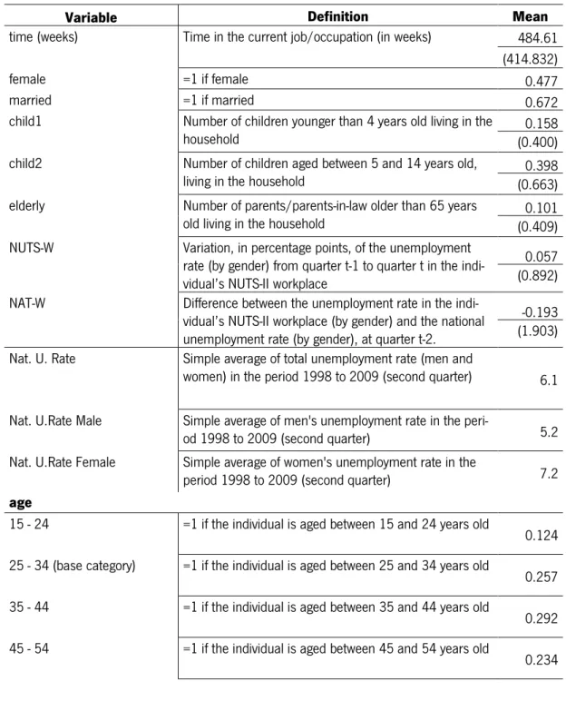
Table 1 presents the descriptive statistics and the variables definition considering the sample to be used on the transition from employment to unemployment. There are 119585 individuals in the sample, corresponding to 362,465 observations. About 47.7% are female and 67.2% are mar-ried. The average age is 38 years, and individuals aged between 35 and 44 years old represent about 29% of the sample. About 30% have the basic 1 level of education, corresponding to four years of schooling, and 27% have at least a high school diploma. The North region is the one with more observations, accounting for 28.6% followed by Lisbon region with 17.9%. On average, the tenure (time) is 484 weeks (about 9.4 years) with a maximum of 1601 weeks (about 30.7 years).
Table 1 – Descriptive statistics and variable definition: From employment to unemployment
Variable Definition Mean
time (weeks) Time in the current job/occupation (in weeks) 484.61 (414.832)
female =1 if female 0.477
married =1 if married 0.672
child1 Number of children younger than 4 years old living in the
household (0.400) 0.158
child2 Number of children aged between 5 and 14 years old,
living in the household (0.663) 0.398 elderly Number of parents/parents-in-law older than 65 years
old living in the household (0.409) 0.101 NUTS-W Variation, in percentage points, of the unemployment
rate (by gender) from quarter t-1 to quarter t in the indi-vidual’s NUTS-II workplace
0.057 (0.892) NAT-W Difference between the unemployment rate in the
indi-vidual’s NUTS-II workplace (by gender) and the national unemployment rate (by gender), at quarter t-2.
-0.193 (1.903) Nat. U. Rate Simple average of total unemployment rate (men and
women) in the period 1998 to 2009 (second quarter) 6.1 Nat. U.Rate Male Simple average of men's unemployment rate in the
peri-od 1998 to 2009 (second quarter) 5.2
Nat. U.Rate Female Simple average of women's unemployment rate in the
period 1998 to 2009 (second quarter) 7.2
age
15 - 24 =1 if the individual is aged between 15 and 24 years old
0.124 25 - 34 (base category) =1 if the individual is aged between 25 and 34 years old
0.257 35 - 44 =1 if the individual is aged between 35 and 44 years old
0.292 45 - 54 =1 if the individual is aged between 45 and 54 years old
21
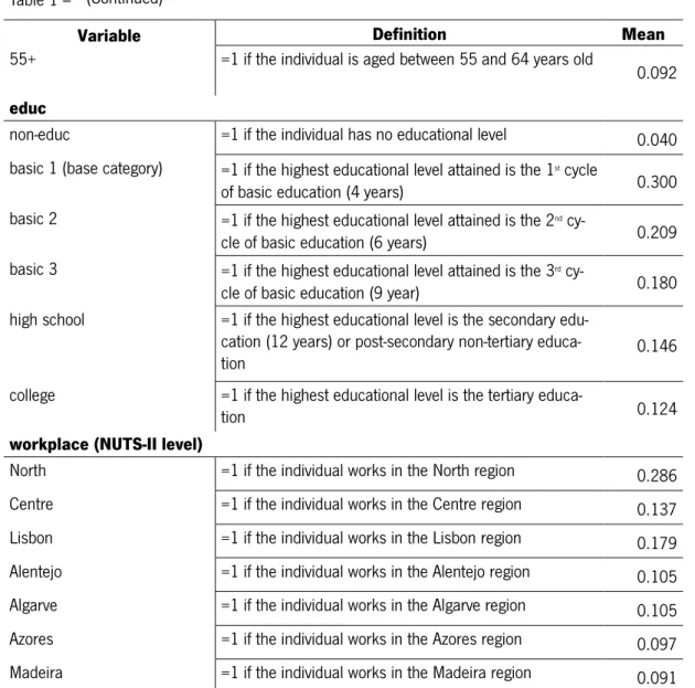
Table 1 – Descriptive statistics and variable definition: From employment to unemployment
Variable Definition Mean
55+ =1 if the individual is aged between 55 and 64 years old
0.092
educ
non-educ =1 if the individual has no educational level 0.040 basic 1 (base category) =1 if the highest educational level attained is the 1st cycle
of basic education (4 years) 0.300
basic 2 =1 if the highest educational level attained is the 2nd
cy-cle of basic education (6 years) 0.209 basic 3 =1 if the highest educational level attained is the 3rd
cy-cle of basic education (9 year) 0.180 high school =1 if the highest educational level is the secondary
edu-cation (12 years) or post-secondary non-tertiary
educa-tion 0.146
college =1 if the highest educational level is the tertiary
educa-tion 0.124
workplace (NUTS-II level)
North =1 if the individual works in the North region 0.286 Centre =1 if the individual works in the Centre region 0.137 Lisbon =1 if the individual works in the Lisbon region 0.179 Alentejo =1 if the individual works in the Alentejo region 0.105 Algarve =1 if the individual works in the Algarve region 0.105 Azores =1 if the individual works in the Azores region 0.097 Madeira =1 if the individual works in the Madeira region 0.091 Note: Standard deviation in parenthesis
4.2.2 From unemployment to employment
The model used to estimate the cause-specific hazard of employment is quite similar to the one
presented before, with some additional variables. Namely, we add a covariate called first, a
dummy variable that indicates whether the individual is looking for her first job, which is a rele-vant variable particularly for the youngest individuals.
As presented in the literature, the job search intensity plays a non-negligible role determining the success of finding a job and leave unemployment status. We add a proxy to job search intensity, the number of active different methods used, in the previous quarter, to find a job (see Riddell and Song, 2011a). We also add the unemployment benefits, to check whether those receiving unemployment assurance in the previous quarter are more prone to remain unemployed. Finally,
22
covariates NUTS-W and NAT-W, from the previous model, where replaced by NUTS-R and NAT-R, respectively. The latter are equal to the former in the way they were computed, with the difference that NUTS-R and NAT-R now use the residence area, rather than the workplace area. Firstly, be-cause we do not have detail about the former workplace area for all unemployed individuals, and secondly, residence area is a better reflection employment prospects for unemployed individuals.
x𝛽 = 𝛽 𝐹𝑒 𝑒 𝛽 𝑀 𝑖𝑒 𝛽 𝐶ℎ𝑖 1 𝛽𝐶ℎ𝑖 𝛽 𝑒
𝐹𝑒 𝑒 (𝛽 𝑀 𝑖𝑒 𝛽 𝐶ℎ𝑖 1 𝛽 𝐶ℎ𝑖 𝛽 𝑒 ) 𝛽 𝛽 𝑒 𝛽 𝐹𝑖 𝑠𝑡 𝛽 𝑏 𝑆𝑒 ℎ 𝛽 𝑒𝑛𝑒𝑓𝑖𝑡𝑠 𝛽 𝑇𝑆 𝛽 𝑇
4.2
Formally, the variables in the model are described in the equation 4.2, as before, a constant may be directly added to the model or be assumed implicitly.
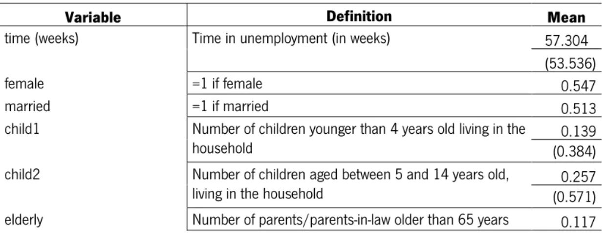
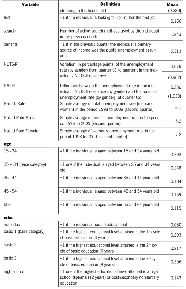
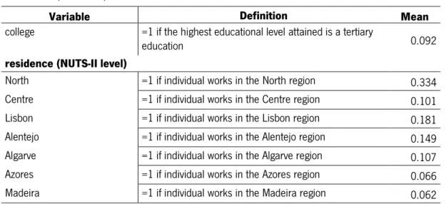
Table 2 presents the descriptive statistics for the data to be used in the study on the transition from unemployment to employment. The sample is composed by 16096 individuals, correspond-ing to a total of 29145 observations. About 54.7% are female and 51.3% are married; the average age is 35 years old. Concerning to education, 29.3% have the basic 1 level while 23.5% have a high school diploma or higher. The region with more observations is the North (33.4%) followed by Lisbon (18.9%). The average duration of unemployment is about one year (i.e. 57 weeks) with a maximum of over 5 years (280 weeks).
We should add that covariates regarding the number of children and elderly living in the house-hold are computed based on the parental relationships and the individuals’ age. Due to some error in variables like age and the missing follow-up for some members of the family, these varia-bles were estimated only for families with complete records for all members.
Table 2 – Descriptive statistics and variable definition: From unemployment to employment
Variable Definition Mean
time (weeks) Time in unemployment (in weeks) 57.304
(53.536)
female =1 if female 0.547
married =1 if married 0.513
child1 Number of children younger than 4 years old living in the
household (0.384) 0.139
child2 Number of children aged between 5 and 14 years old,
living in the household (0.571) 0.257 elderly Number of parents/parents-in-law older than 65 years 0.117
23
Table 2 – Descriptive statistics and variable definition: From unemployment to employment
Variable Definition Mean
old living in the household (0.389)
first =1 if the individual is looking for (or in) her the first job
0.166 search Number of active search methods used by the individual
in the previous quarter 1.843
benefits =1 if in the previous quarter the individual's primary source of income was the public unemployment
assur-ance 0.313
NUTS-R Variation, in percentage points, of the unemployment rate (by gender) from quarter t-1 to quarter t in the indi-vidual’s NUTS-II residence
0.075 (0.962) NAT-R Difference between the unemployment rate in the
indi-vidual’s NUTS-II residence (by gender) and the national unemployment rate (by gender), at quarter t-2
0.260 (1.930) Nat. U. Rate Simple average of total unemployment rate (men and
women) in the period 1998 to 2009 (second quarter) 6.1 Nat. U.Rate Male Simple average of men's unemployment rate in the
peri-od 1998 to 2009 (second quarter) 5.2
Nat. U.Rate Female Simple average of women's unemployment rate in the
period 1998 to 2009 (second quarter) 7.2
age
15 - 24 =1 if the individual is aged between 15 and 24 years old
0.293 25 – 34 (base category) =1 one if the individual is aged between 25 and 34 years
old 0.248
35 - 44 =1 if the individual is aged between 35 and 44 years old
0.184 45 - 54 =1 if the individual is aged between 45 and 54 years old
0.159 55+ =1 if the individual is aged between 55 and 64 years old
0.115
educ
non-educ =1 if the individual has no educational 0.050 basic 1 (base category) =1 if the highest educational level attained is the 1st cycle
of basic education (4 years) 0.293
basic 2 =1 if the highest educational level attained is the 2nd
cy-cle of basic education (6 years) 0.217 basic 3 =1 if the highest educational level attained is the 3rd
cy-cle of basic education (9 years) 0.206 high school =1 one if the highest educational level attained is a high
school diploma (12 years) or post-secondary non-tertiary
education 0.143
24
Table 2 – Descriptive statistics and variable definition: From unemployment to employment
Variable Definition Mean
college =1 if the highest educational level attained is a tertiary
education 0.092
residence (NUTS-II level)
North =1 if individual works in the North region 0.334 Centre =1 if individual works in the Centre region 0.101 Lisbon =1 if individual works in the Lisbon region 0.181 Alentejo =1 if individual works in the Alentejo region 0.149 Algarve =1 if individual works in the Algarve region 0.107 Azores =1 if individual works in the Azores region 0.066 Madeira =1 if individual works in the Madeira region 0.062 Note: Standard deviation in parenthesis
25
5
Results and discussion
In this section, we present the results for cause-specific hazard (single risk). Section 5.1 refers to the transition from employment to unemployment model, whereas in Section 5.2 we present the estimation results for the unemployment to employment model.
We also estimate the cumulative incidence function, CIF, (competing risks) that yield similar re-sults as those found in this section; the rere-sults can be found in appendix C.
5.1 From employment to unemployment
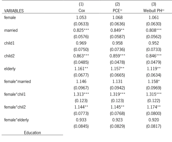
Table 3 presents the estimation results for the cause-specific hazard of unemployment (single risk), for three alternative models (Cox PH, PCE and Weibull PH), that yielded quite similar esti-mates for all models.
All models were estimated considering stratification by economic activity28 using the Stata®
com-mand strata, except the PCE model where the stratification was made by adding a dummy varia-ble for each economic activity (omitted from the output). In the PCE model, model 2, we try dif-ferent time intervals, and use the Akaike Information Criterion to choose the optimal time vals. Our final choice was intervals of 52 weeks up to week 520 (ten intervals), 260 weeks inter-vals onwards up week 1560 (30 years), and a final interval for more than 30 years. In the Weibull PH model estimation, model 3, we omitted the ancillary estimators for each stratum, for a matter of space and readability. Also note that robust standard errors were used, allowing for intragroup correlation within the household (family), i.e., the observations are considered independent across households but correlated within the household. For those aged between 45 and 54 a time interaction was added by the mean of two dummies, one for those working form less than 1300 weeks (25 years) and other for those working for more than 25 years. The purpose of these interactions is to guarantee that proportional hazard rate was not violated, as preliminary estima-tions suggested.
The results show that single women have a higher risk of job loss comparing to men (5.3% in Cox model), although the estimators are not significant at 10% for all models. Regarding to marital status, the difference between married men and married women is given by:
26
𝑛[ℎ(𝑡| 𝑓𝑒 𝑒 = 1, 𝑖𝑒 = 1) − ℎ(𝑡| 𝑓𝑒 𝑒 = 0, 𝑖𝑒 = 1)]
= (𝛽 𝛽 𝛽 ) − (𝛽 ∗ 0 𝛽 𝛽 ∗ 0) = 𝛽 𝛽
The estimated result for Cox model is 1.2067 with Wald statistic of 7.23, significant at a 1% level. Comparing married men with single ones, the former have lower risk of unemployment: 17.5% in the Cox model and 19.2% in the Weibull PH model. Married women do not significantly differ from single women (10% level).
Our results suggest that the family structure plays an important role to the transition to unem-ployment, and affects men and women differently. A joint test for covariates child1, chil2 and el-derly show that they are statistically relevant at 1% in Cox and Weibull PH models in the likeli-hood-ratio test29,30:
Table 3 – Cause-specific hazard of unemployment estimation results31
(1) (2) (3)
VARIABLES Cox PCE32 Weibull PH33
female 1.053 1.068 1.061 (0.0633) (0.0636) (0.0630) married 0.825*** 0.849** 0.808*** (0.0576) (0.0587) (0.0562) child1 0.969 0.958 0.952 (0.0750) (0.0736) (0.0733) child2 0.863*** 0.859*** 0.846*** (0.0485) (0.0478) (0.0479) elderly 1.161** 1.157** 1.119** (0.0677) (0.0665) (0.0634) female*married 1.146 1.131 1.158* (0.0967) (0.0942) (0.0969) female*chil1 1.313*** 1.319*** 1.315*** (0.123) (0.123) (0.122) female*chil2 1.144** 1.145** 1.174** (0.0773) (0.0768) (0.0800) female*elderly 0.933 0.923 0.920 (0.0845) (0.0829) (0.0817) Education
29 ( ) = 9 (p<0.01) for Cox model, and ( ) = (p<0.01) for Weibull PH model. 30 In order to perform the test, we have to estimate the models without robust standard errors.
31The results are presented in the form of hazard ratio, where values above 1 mean a higher hazard and values below 1 indicate
a lower hazard of transition.
32The model specification also included variables such as the time dummies and the stratum dummies, which results have not
been reported for simplicity reasons.