M
ESTRADO EM
A
CTUARIAL
S
CIENCE
T
RABALHO
F
INAL DE
M
ESTRADO
I
NTERNSHIP
R
EPORT
N
EW
C
REDIBILITY
A
PPROACHES IN
W
ORKERS
C
OMPENSATION
I
NSURANCE
J
OÃO
P
EDRO
S
ENHORÃES
S
ENRA
P
INTO
ORIENTAÇÃO:
P
ROFESSORJ
OÃOA
NDRADE ES
ILVAD
IRETORR
UIA
LEXANDRES
ILVAE
STEVESI would begin by thanking Fidelidade for the opportunity to develop my master final work in such a
prestigious institution. On a personal level, I’d like to express my gratitude to Director Rui Esteves,
not only for his very helpful insights, but also for the enormous freedom given, which allowed me
to achieve a much deeper understanding of the recent advances in the ratemaking process. Also
to Director Delminda Rangel, always available to help with every doubt and every request, and to
all the wonderful team at DET, in particular Patrícia Neto, Mário Nogueira and Maria João
Cartaxana for their instructive remarks about the functioning of workers compensation insurance
and to Catarina Jácomo who was always extremely helpful, especially with the informatics. I would
also like to thank my fellow intern Tiago Fardilha for the exchange of ideas during the time of our
internship.
Regarding the scientific component of this work, I would like to extend my sincere thanks to Prof.
João Andrade e Silva for his enormous availability and the valuable guidance. I would also like to
thank Prof. Lourdes Centeno, for all the precious help at different moments in the master.
My wife, daughter, and son I would like to immensely thank for their understanding and apologise
for the moments when my attention was disputed by my internship work, the redaction of this report
and the study for some exams, which prevented me to be the husband and father they deserve.
Finally, I would like to remember two great women, my grandmother and my godmother, who died
during this master. I miss you.
Abstract:
In our report, several interpretations of Bühlmann credibility are applied in the workers
compensation portfolio of a portuguese insurance company. We begin with classical
implementations of Bühlmann-Straub and Jewell models, and then we display a more recent
reading of those models as Linear Mixed Models. We end presenting two approaches that show
how Bühlmann credibility can enhance the performance of generalized linear models.
Key words: Credibility, Generalized Linear Models, Mixed Models, Workers Compensation,
Ratemaking.
Resumo:
No nosso relatório apresentamos diferentes interpretações da teoria de credibilidade de Bühlmann
que foram aplicadas na análise da carteira de seguros de trabalho de uma seguradora portuguesa.
Começamos pela apresentação e implementação dos modelos clássicos de Bühlmann-Straub e
Jewell, posteriormente debruçamo-nos sobre a mais recente leitura destes modelos enquanto
modelos lineares mistos. Por fim, apresentamos duas abordagens que sugerem como a
credibilidade de Bühlmann poderá aperfeiçoar o desempenho dos modelos lineares generalizados.
Palavras chave: Credibilidade, Modelos Lineares Generalizados, Modelos Mistos, Seguro de
Índice
Introduction ... 1
1. Classical credibility ... 3
1.1. The Bühlmann-Straub model ... 4
1.2. Hierarchical model ... 5
1.3 Some notes about credibility estimation in the hierarchical model ... 6
1.4. Example of model application ... 8
1.5. A costumer’s perspective, credibility as negotiation tool ... 12
1.6. Regression model of Hachemeister ... 13
2. Credibility via linear mixed models ... 14
2.1. Linear Mixed Models in the credibility framework ... 15
2.2. Model application: Bühlmann model ... 16
2.3. Model application: BS model ... 17
2.4. Model application: Hierarchical model. First level: CAE, Second level: Sector ... 19
2.5. Some final relevant notes ... 20
3. Credibility and generalized linear mixed models ... 21
3.1. From GLM to GLMM´s ... 22
3.2. Model application: 2014 losses ... 23
3.3. Model application: forecasting the number of claims ... 28
Conclusion ... 34
References ... 36
Annex 1: Assumptions of the Jewell model... 38
Annex 2: BS and LM models: a theoretical approach ... 39
Annex 3: Complementary results to access the quality of the forecasting ... 41
P á g i n a 1 | 46
Subiu a construção como se fosse sólido Ergueu no patamar quatro paredes mágicas Tijolo com tijolo num desenho lógico (…) E tropeçou no céu como se ouvisse música E flutuou no ar como se fosse sábado
Chico Buarque in «Construção»
Introduction
«Construção» is probably one of the best known Buarque´s songs. The tense horns arrangement
sets the scenario to the haunting story of the death of a construction worker, falling from the building
where he was working. The listener is promptly confronted with the dramatic effects those accidents
could have in the workers and also in their families.
As far as we can see, there are two ways to mitigate those effects: improve the safety conditions
of the companies in order to diminish the probability (and severity) of accidents and gave to the
injured workers a fair compensation for the damages suffered at work. Obviously, both approaches
imply generally important costs. To a less attentive sight, the role of an insurance company is
exclusively related with the financial compensation and correction of the damage of part of those
costs: the insurer should pay the legal compensation to the workers and, in order to do so, a
premium should be collected. The calculation of this premium should reflect some stablished
risk-related features of each client, like the kind of activity developed, dimension of business and so on.
Roughly, this is the definition of the a priori approach to the ratemaking process.
But what if we could also include in the process the noble propose of improving the security of work
environment? This could be done taking in account the claim record of each company. Ideally,
having this information, it would be possible to reward responsible behaviours of the employers
P á g i n a 2 | 46
ratemaking; when successfully applied, allow a more competitive intervention in the market, offering
attractive conditions to retain the so called good risks. Also, it could act as a complement to the
intervention of workers conditions authorities, since charging more severely the companies with a
problematic claim record (considering what was expected for the line of business) should give an
incentive to improve the general working conditions, so in a certain way all the society could benefit
from this effort.
That fascinating challenge was the base of our internship. During five months, we have the
opportunity to research some of the latest developments related with this fundamental problem.
Also, we have the chance to apply those techniques to the biggest policy portfolio in the Portuguese
market. This report includes some of our more important findings although it isn´t completely
exhaustive. We have privileged a practical approach, more focused in the model applications and
the discussion of results.
In this work we try to describe some of the several ways to approach the experience rating using a
fundamental actuarial tool: the credibility theory. In Chapter 1, we review the most usual
applications of credibility theory in workers compensation. We present the classical models of
credibility and apply them to a real life portfolio, we also compare and discuss some results.
Chapter 2 is dedicated to a more recent interpretation of the classical credibility models as linear
mixed models. We explore briefly the theoretical link between the concepts and conduct some
comparative experiences that strengthen our theoretical approach.
Finally, in Chapter 3, we try to show one of the most promising lines of research in this area. The
idea is to use the link stablished in Chapter 2 in order to introduce the credibility in the context of
the most important tool in the a priori ratemaking: Generalized Linear Models. We develop an
experience that gave promising results, but computational issues didn´t allowed us to generalize it
to the policy level as we wished. Instead, we design a slightly different two step method that
combines also GLM and credibility. The method was later applied in a predictive task.
P á g i n a 3 | 46
1.
Classical credibility
There is nothing particularly disruptive on the idea of using the credibility theory in context of
workers compensation (as it is explained in Goulet (1998) which we will follow closely in this
section). As a matter of fact, the birth of this approach to the experience ratemaking is usually
associated with a 1914 paper published by A.H. Mowbray where the author describes a method to
find the number of employees needed to get a reliable (or credible) and, more important in this
framework, stable estimate of the Premium to be charged. The ideas of Mowbray were developed
in Whitney’s influential paper “The theory of experience rating”, where for the first time appears the
classical formulation:
(1) 𝑃𝑐 = 𝑧𝑋 + (1 − 𝑧)𝑚.
Speaking in terms of actuarial practice: this formula states that the credibility premium (𝑃𝑐) comes
from a compromise between the individual’s experience (𝑋) and the collective mean (𝑚), an interpretation to which we will return many times in this report. The weighing between those two
amounts (𝑧) - the credibility factor -, still according with Whitney’s calculations, should be established by an expression of the form:
(2) 𝑧 = 𝑛 + 𝐾 .𝑛
In this expression n could be, for instance, the number of periods of experience and K a constant,
although not an arbitrary constant, but rather an explicit expression that should reflect some main
features of the model. The role of this constant is quite central in credibility theory and some of the
great developments in this field are related to innovative approaches in the best way to determinate
it’s value. For instance, traditionally, last century American actuaries usually privileged the stability of premia, so in practice the value of K was establish mainly by actuary judgment. In Europe, a
very influential 1967 paper published by Hans Bühlmann proposed another direction. In the now
P á g i n a 4 | 46
(3) 𝐾 =𝑠𝑎 .2
Although Bühlmann reaches this expression after rigorous calculations, the result obtained is also
very intuitive and easy to explain avoiding extensive formalization. As we shall see with more
detail, 𝑠2 could be seen as a global measure of within variance or heterogeneity within insureds.
On the other hand, 𝑎 will work as an indicator of heterogeneity among insureds. Returning to (2),
we get the whole picture: as the value of 𝑠2, or, equivalently, the heterogeneity in the individual
experience, increases, the less reliable will be historical behavior of the client, as a consequence
value of the credibility factor will drop. Conversely, when the heterogeneity between insureds
increases, the less important will be the collective behavior in the evaluation of a particular client,
so the value of the credibility factor, and the weight of individual experience, should grow.
Bühlmann´s ideas still very influenting even today, being a major cornerstone not only on the
experience rating but also in other actuarial fields like loss reserving. More, the plasticity and
robustness of the original model gave rise to numerous variations and generalizations, some of
them, as we will shall see, extremely surprising and unexpected. The most famous of those,
introduced in 1970 as a tool to rate reinsurance treaties, is the Bühlmann-Straub model.
1.1. The Bühlmann-Straub model
As expected, given that was originally developed to reinsurance treaties, the Bühlmann-Straub
model great innovation was its attention to the questions related with the volume. Roughly, this
model joint to the original framework the notion of weights, which can be interpreted as any valid
measure of exposure. In workers compensation framework, for example, some acceptable
measures of risk exposure could be: Capital insured, the total number of workers, or the total payroll
in that year, among many others. In our notation, 𝑊𝑖𝑡 will mean the exposure of the risk 𝑖 at time 𝑡.
In an equivalent approach, 𝑋𝑖𝑡 will represent the relevant information of claims experience (like
P á g i n a 5 | 46
inversely proportional to 𝑊𝑖𝑡 . We will also define 𝜃𝑖, which can be understood as an unobservable
parameter representing the specific profile of the risk 𝑖.
The robustness of Bühlmann-Straub model depends in a large measure of the practical validity of
the following mathematical assumptions:
BS1: Given 𝜃𝑖 the vector of realizations 𝑋̅̅̅̅ = (𝑋𝑖 𝑖1, 𝑋𝑖2,… , 𝑋𝑖𝑇𝑖), 𝑖 = 1,2, … 𝐼 are mutually
independent.
BS1’:The following moments exist: 𝐸[𝑋𝑖𝑡|𝜃𝑖] = 𝑢(𝜃𝑖), 𝑉𝑎𝑟[𝑋𝑖𝑡|𝜃𝑖] =𝜎2(𝜃𝑖)
𝑊𝑖𝑡 .
BS2: (𝑋̅1, 𝜃1), (𝑋̅2, 𝜃2), … , (𝑋̅𝐼, 𝜃𝐼) are independent.
BS3: 𝜃1, 𝜃2, … , 𝜃𝐼 are i.i.d generated by a distribution 𝑈(𝜃) .
It is important to point out, returning to a terminology already used, that assumption BS1 is related
with noncorrelation within the risks while BS2 is connected with the independence between the
risks.
Now that the fundamentals of the model were stated, we can return to equations (1) , (2) , (3), in
the light of Bühlmann-Straub approach. As usual in practical context, this could be done choosing
the most adequate estimators of the quantities of interest, in this case 𝑚, 𝑠2 and 𝑎, a subject to
which we will return later.
1.2. Hierarchical model
In large and very heterogeneous portfolios, like the one we were assign in our internship, the choice
of Bühlmann-Straub model could generate some questions. For instance, we can think in scenario
were a policyholder with a very small credibility factor, could have a Premium resulting almost
exclusively by a collective which shares very little with him. Also, Bühlmann-Straub assumptions
seem to restricting, ignoring important collateral information that could be useful in the evaluation
of several risks. In a certain way, the model interprets the portfolio structure like it was a single
P á g i n a 6 | 46
The hierarchical model, initially developed by W.S Jewell in a 1975 paper, could be seen as an
effort to solve those questions within the framework of credibility. Essentially, the idea is to divide
the portfolio in large subsections that share some feature believed to be important to the risk
evaluation process. The classical example in workers compensation insurance is to divide the
different companies in classes of economic activities. Other approach could be divide the policies
by geographical region, and many others similar ideas could be developed. Also, the model is
flexible enough to allow the inclusion of more levels of segmentation. If it is believed, for instance,
that the portfolio still very heterogeneous even after the segmentation in economic classes, we can
create another hierarchical level, of sectors, that aggregate related economic classes. As obvious,
this process could be repeated several times.
In the simplest formulation, the model assumes the existence of three hierarchical levels. Level 3
is the entire portfolio; this portfolio will be divided in sectors: the main constitution of level 2. The
risk features of the pth sectorare described by 𝜓𝑝 for p=1,…,P, assumed to be a realization of a random variable Ψ. At level 1, where each unit consists in homogeneous policies, the risk features
of each policy i within the sector p are characterized by 𝜃𝑝𝑖 , i=1,…, I, assumed to be a realization
of (𝜃| 𝜓𝑝). As is pointed in Concordia (2000), it is interesting to see that although the risk
parameter of each sector can take a different, specific, value, they all came from the same
distribution. This kind of formulation emphasizes the main strength of the hierarchical model: accept
the individuality of different participants (introduced by the different risk levels to each sector) in a
structural design that highlights their homogeneity (established by their common distribution). The
assumptions of this model, closert to the ones already presented to the BS model, could be found
in annex 1.
1.3 Some notes about credibility estimation in the hierarchical model
As Goulet (1998) points out, both BS and hierarchical model, while similar in many aspects, are
P á g i n a 7 | 46
each sector separately isn´t equivalent to apply the hierarchical model, as some distracted
evaluation may suggest. The first approach, although theoretically valid, assumes that all sectors
are mutually independent, in others words, express believe that there isn´t useful information in the
policies outside the sector we are interested in. The hierarchical method, on the other hand,
expresses a different point of view, where all the policies embrace some collateral ratemaking
information that should be used in the evaluation of every sector. The choice between both models
should express our prior believes about the data we are analysing.
Although both models reflects a very different understanding of the nature of a portfolio, they share
a almost equivalent approach in the calculation of the homogeneous credibility estimators. Even
though it is a very interesting topic, we will avoid mathematical demonstrations or longest
discussions about this subject, there are plenty of other texts that cover the subject in detail, for
instance: Belhadad (2009), we limitate our analysis to the basics features.
Essentially, in the hierarchical model1, the estimation of the risk premium will be a recursive process
of the type:
𝑋𝑝𝑖,𝑇𝑖+1= 𝑧𝑝𝑖𝑋̅𝑝𝑖∎+ (1 − 𝑧𝑝𝑖)[𝑧𝑝𝑋̅𝑝∎∎+ (1 − 𝑧𝑝)𝑚].
The credibility factors are:
𝑧𝑝𝑖= 𝑊𝑝𝑖∎
𝑊𝑝𝑖∎+ 𝑠2𝑎
with 𝑊𝑝𝑖∎ = ∑𝑇𝑖𝑡=1𝑊𝑝𝑖𝑡
and
𝑧𝑝 = 𝑍𝑝∎
𝑍𝑝∎+ 𝑎𝑏 with 𝑧𝑝∎ = ∑ 𝑧𝑝𝑖
𝐼 𝑖=1 .
Also, the weighted averages are given by:
𝑋̅𝑝𝑖∎ = ∑ 𝑊𝑝𝑖𝑡
𝑍𝑝𝑖∎
𝑇𝑖
𝑡=1 𝑋𝑝𝑖𝑡 and 𝑋̅𝑝∎∎ = ∑𝐼𝑖=1𝑍𝑧𝑝∎𝑝𝑖 𝑋𝑝𝑖∎.
Regarding the estimation of the structural parameters, there are several options available and in
our practical work at Fidelidade we´ve tried (via R package “Actuar”) with three different kinds of
1 The BS estimates, as is known, could easily be obtained from these expressions suppressing the
P á g i n a 8 | 46
estimators: the classical Iterative pseudo-estimator, Bühlmann-Gisler and Olhsson estimators. In
the model applications below, we´ve struggle to decide either to present the results obtained with
the iterative estimator or the Bühlmann-Gisler estimator. The iterative method is definitely our
favourite due to its intuitiveness and stability of results, but in the other hand Bühlmann-Gisler
methodology is more consistent with the nature of subjects developed in chapter 2. Finally we
decided to present the results with the iterative estimator in Chapter 1, since it seems less
vulnerable to one of the main difficulties of our portfolio: aggregate policies that were in force just
some few weeks with policies that stand eight years with the company. In Chapter 2 and 3 we
have used the unbiased estimators of Bühlmann-Gisler.
1.4. Example of model application
We were fortunate enough to get at our disposal the data of an enormous and very heterogeneous
portfolio, with more than 300000 workers compensation policies, and information related with a
time period from 2007 to 2014. We won´t describe in detail the main features of this data since a
fair part of it will be illuminated in subsequent sections of our work.
We have performed several different analysis to the data using the presented models of credibility.
We applied them to the analysis of the frequency and the severity of the claims, for instance, but
will present here only the results regarding the most traditional approach to ratemaking. In this
context, we will take as exposure measure 𝑊𝑖𝑡: the capital insured for risk i at year t. 𝑋𝑖𝑡 will be
defined as the ratio between the aggregate claim amount and capital insured where the subscripts
have the same interpretation.
Besides information about claim cost and number of claims, our data includes also several
indications of the professional activity related with each policy. This segmentation includes three
P á g i n a 9 | 46
some considerations must be made. When we are dealing with this kind of structure, we hope that
the classes of individuals could be somehow homogeneous, meaning that they were able to
aggregate some important features of the risk level. On the other hand, we hope that the situation
could be reversed in hierarchical level above: very homogeneous sectors could signalize an
insufficient number of classes or that the classes existent are too similar. There is nevertheless a
small downsize in this kind of data aggregation: it isn´t fully compatible with one of the main
challenges of our internship - try to develop our analysis in a customer’s perspective. As a matter of fact, we realized that several customers had policies in different CAE´s and sectors, and although
some adaptations were tried, none seemed to be completely convincing; as consequence, we
decided to adopt the policy at the most elementary object in the hierarchical structure.
In this report, we will only present a comparative analysis of the following models: BS model applied
to the policies, Jewell model with one hierarchical level (CAE) and also a model taking in account
two hierarchical levels: CAE and sector. Our goal will be the study of the ratio between the total
losses of each policy and an exposure measure (Capital insured). An important note should be
made: we decided to exclude the policies that were in force a single year. As it is explained with
some detail in Concordia (2000), there is an asymmetric effect of this kind of policies in the value
of within variance and between variances that could compromise the quality of the results and
comparisons. Also we have bounded to 20 the largest ratio, otherwise the variability of the portfolio wouldn´t allowed us to truly take advantage of the credibility framework. This option could be
controversial. As Bühlmann and Gisler (2005) argued this kind of truncation is incompatible with
BS assumptions since the biggest companies will have a smaller chance to get to the truncation
point, and so 𝐸[𝑋𝑖𝑡|𝜃𝑖] = 𝑢(𝜃𝑖) will also depend on the volume wij. We believe, nevertheless,
that our approach is valid since the biggest ratios are usually related with very small policies with
an unlikely value of capital insured.
P á g i n a 10 | 46
Collective premium: 0.017083542
Between policy variance: 0.0004834807 Within policy variance: 438.7385
In the one level hierarchical model:
Collective premium: 0.01791848 Between CAE variance: 0.0001612929 Within CAE/Between policy variance: 0.0003376572
Within policy variance: 438.7385
Finally, in the two level hierarchical model:
Collective premium: 0.017328 Between Sector variance: 0.0001137691 Within Sector/Between CAE variance: 0.0001262442
Within CAE/Between policy variance: 0.0003376572 Within policy variance: 438.7385
As we have already said, the models represent a different interpretation of the features of our
portfolio, so we shouldn´t be concerned about which model is more correct. A different, and possibly
more interesting, question is «Are some of those models somehow redundant?». For instance, a
classical question: the inclusion of a third level justifies all the extra computational effort? In our
view, the answer is negative, although our opinion doesn´t seek explanation in the computational
issues, less problematic these days. We justify our answer with an analysis of the differences
between credibility premia obtained in Policy/CAE and in the Policy/CAE/Sector model.
Min. 1st Qu. Median Mean 3rd Qu. Max.
Difference -1.175e-02 6.345e-06 6.471e-06 1.577e-05 2.895e-05 5.555e-03
So both models presented indeed very close projections to the credibility Premium (only for two
policies an absolute difference above 0.01 was obtained). We also want to point out that we are
2 For confidentiality purposes, we could have masked some values in different sections of our work. That
procedure, as obvious, doesn´t had any impact in our conclusions.
Table I – Summary of the differences between the credibility premiums suggested by the two
P á g i n a 11 | 46
aware of rudimentary nature of the tools used in the comparison of the models, seemingly much
unsophisticated when compared with all the arsenal of hypothesis testing available in the
regression environment; we will try to present strategies to close this gap in Chapter 2.
Regarding the comparison between BS model / one level hierarchical model the results aren´t so
clear.
Min. 1st Qu. Median Mean 3rd Qu. Max.
BS-hierarchical -0.0625800 -0.0020970 0.0070770 0.0007732 0.0074300 0.0900700
Now we see important differences that enlighten the dissimilar nature of models. For instance,
regarding the minimum value observed, we have checked that it corresponds to a policy in CAE 20
(forestry) which has a credibility premium of 0.07971. A deeper look showed that all the situations
where the credibility premium of the hierarchical model exceed in 0.05 the one proposed by the BS
model (898 in total) were actually policies from the same CAE. It isn´t difficult to figure out what has
happened: CAE 20 is a very heterogeneous CAE with a within variance equal to 0.06510139,
almost 200 times more than the average between CAE variance in the Portfolio. As a consequence,
a lot of policies, especially those with small capital insured which leads to a small credibility factor,
will see their Premium highly penalized by the credibility Premium of the CAE, which in this case is
almost 0.08; in the BS model the counterpart to their individual experience will be 0.017 and the
compromise between those two amounts will lead generally to a smoother risk perception. In face
of those results we are tempted to suggest a segmentation of this CAE in smaller, more
homogenised, units.
The other extreme value of the table II is related with a different effect: here we are talking about
a policy with a quite extreme average ratio equal to 3.882571, as consequence, since the BS model
gives more credit to the individual experience, the projected credibility Premium won´t be so kind
to the policyholder.
Table II – Summary of the differences between the credibility premiums suggested by the BS and the
P á g i n a 12 | 46
1.5. A costumer’s perspective, credibility as negotiation tool
We also have tried a different approach. During our first days in internship we´ve analysed some
figures describing the bonus that the companies were able to obtain regarding the reference tariff.
We´ve seen, for instance, that the companies called “Dominantes” (with capital insured above 5000000) get much more generally important reductions in the value of their premia, which is
absolutely unsurprising since they have an enormous room for negotiation. We´ve wonder if the
Credibility theory could provide some support to this framework, so we´ve applied the BS model,
having the costumer as risk unit. Aggregating all the policies associated with a particular client (we´ve
excluded the policies without number of clients and again the temporary policies) we get the following
results:
Collective premium: 0.01679245 Between Costumer variance: 0.0002581788
Within Costumer variance: 441.2156
Then we´ve reversed the reasoning of the previous model applications, our goal now is try to find
the dimension (using capital insured as measure) that a company must have in order to achieve
certain credibility factors:
So, as we can see, and since we are following a eight year span, a company insured in all this
period with an Capital Insured above 32470119/8= 4058764 year, has the “right” to claim a Premium determined essentially by the Individual mean. This value isn´t that different from the one
suggested by the definition of “Dominantes” costumers, although we´ve pointed this out just as a
C. F Dimension
0.75 5 126 861
0.85 9 684 071
0.9 15 380 583
0.95 32 470 119
Table III – Credibility factor as a
P á g i n a 13 | 46
curiosity, our aim isn´t to state the efficiency of this market or something related (among others
reasons, the value obtained is very sensible even to slight changes in the variances).
1.6. Regression model of Hachemeister
We would like to close this chapter with a brief reference to the model introduced by Hachemeister
in 1975, who have use it in the analysis of the inflation in body insurance claims of five different
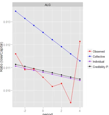
American States. The great innovation of this model was the incorporation of a linear trend – a regression model. Only as an example, we have run a naive implementation of this model in our
data, using the geographical region as the risk unit. Here, we will present only the scenario in
Algarve. The y-axis measures the ratios between losses and capital exposure, on the horizontal
axes it´s an indication of time which was centred in 2010 (which means: period = year of
development – 2010).
The red line connects the ratios observed in the period considered. The blue line presents the trend
if all the geographical regions were considered together; is an equivalent of the collective Premium
P á g i n a 14 | 46
of the previous models. The purple line incorporates a specific intercept and slope for each region,
so acts as the individual component of the credibility model. Finally the black line is a compromise
between the purple and red line, analogous to the credibility Premium. As we can see the predictive
results from this approach are very far from excellent, we decided either way to include it in our
work for two reasons: presents a nice visual interpretation of the concept of credibility and, more
important, was the first deliberate link established between regression and credibility. We will
devote the next sections of our work to the presentation of others links between both subjects.
2. Credibility via linear mixed models
Hachemeister introduction of the regression in the universe of credibility was in a certain way
incidental, probably explained in a major part by the necessity to include the turmoil of the seventies
inflation within the ratemaking process. In a time where the stability of prices seems to be
strengthen, does this connection between regression and credibility still pertinent?
The answer to this question can be traced to the birth of regression itself. The story comes in
hundreds statistics books: Francis Galton´s famous experience interpreting the heights from
children´s using the heights of their parents. The rather famous, although somehow simplified,
conclusion states that, on average, the sons of the taller parents won´t be as tall as their
progenitors; a similar effect should be seen within the shortest families even if in the opposite
direction. Galton described this phenomenon coining the term: «regression to the mean», which he
used interchangeably with the more pessimistic «reversion to the mediocrity». It´s difficult to not
see some familiarity between this concept of regression to the mean and the shrinking towards the
average (credibility) Premium proposed by the credibility models developed in the chapter before.
This link, nevertheless, won´t be established by the more traditional regression models; we will rely
P á g i n a 15 | 46
2.1. Linear Mixed Models in the credibility framework
A Linear Mixed Model (LMM) is nothing other than a classical linear regression model with the
incorporation of the so called “random” effects which should be combined with the usual, now
called, “fixed” effects. In the simplest form we will have something like:
(4) 𝑌𝑖 = 𝑋𝑖𝛽 + 𝑊𝑖𝑢𝑖 + 𝜀𝑖 .
We will describe with more detail each term of this equation but so far we present some short notes.
First, we see that the only major innovation regarding the classical regression model is the inclusion
of the random effects term - in this case 𝑊𝑖𝑢𝑖 - representing subject specific component related,
for instance, with risk profile of a specific policyholder. As usual 𝑋𝑖𝛽 represents the fixed effects of
the independent variables and 𝜀𝑖 an error term with zero mean. Now if we compare this with a
slightly modified version of (1):
(5) 𝑃𝑖 = 𝑍𝑖𝑀𝑖 + (1 − 𝑍)𝑀 = 𝑀 + 𝑍(𝑀𝑖− 𝑀).
We start to get some insight of the dynamics in the process. 𝑋𝛽 will be strongly interconnected
with estimation of M - the grand mean- and the role of the random individual effect, 𝑊𝑖𝑢𝑖, will be
linked to the behaviour of the risk specific deviation 𝑍(𝑀𝑖 − 𝑀).
Following Klinker (2011), we will describe this family of models with more detail. We start with:
(6) 𝑌 = 𝑋𝛽 + 𝑊𝑢 + 𝜀.
If we have n observations, Y is the response vector (for instance, the number of claims), X a n x p
design matrix (representing the structure of the fixed terms); 𝛽 will be a p-vector of parameters
and 𝜀 an error term like in the usual regression model. 𝑢 will have an equivalent role to 𝛽, so will
act like a q-vector of regression coefficients of random effects. W is also a design matrix (n x q) for
the random effects, generally a matrix with 0 and 1 elements, where 𝑊𝑖𝑗=1 if the random effect 𝑢𝑗
as some influence over the observation. Also:
P á g i n a 16 | 46
where G and R are a q x q matrix and n x n matrix respectively; G is usually assumed to be diagonal
with each non zero element equal 𝜎𝑢2. Since u aggregates the subject specific behaviour, it won´t
be surprise if we relate 𝜎𝑢2 with the concept of between variance exploited in the first chapter. R
isn´t necessarily a diagonal matrix, it can be used for instance to allow autocorrelated time series
structure, (see Klugman (2015)), but we can disregard those features in this context, where R is
strongly related with the idea of withinvariance. The nature of our work doesn´t allow us to go much
deeper in the technical discussion but more details can be found in Antonio and Zhang (2014a)
and Frees (2004).
Finally it will also be important for some future results to be aware of the some dichotomy that could
arise from the normal conditional distribution 𝑌|𝑢 with
𝐸[𝑌|𝑢] = 𝑋𝛽 + 𝑊𝑢 and 𝑉𝑎𝑟[𝑌|𝑢] = 𝑅
and the marginal distribution:
𝑦 ~𝑁 (𝑋𝐵, 𝑉 ≔ 𝑊𝐺𝑊′ + 𝑅).
If our interest is limited the fixed effects the marginal model can be used, when there is also explicit
concern in the random effects then we need to look to the conditional distribution.
2.2. Model application: Bühlmann model
We think that we´ve already presented enough arguments stating the similitudes between the
concepts of LMM and credibility. Before discussing theoretically that relation, we will present an
example using the Bühlmann model. In the example presented here we will take the sector of
activity as the risk unit, since it has only seventeen different categories, otherwise the presentation
of results would be very exhausting. The response average will be, again, the ratio between losses
and capital insured, in sector i at year t (as in the first chapter the time range will be 2007/2014).
Following the approach of Antonio and Zhang (2014) we will try to replicate the Bühlmann model
with the following equation:
P á g i n a 17 | 46
with: 𝑢𝑖~𝑁(𝑂, 𝜎𝑢2) 𝑖. 𝑖. 𝑑 and 𝜀𝑖𝑡~𝑁(𝑂, 𝜎𝜀2) 𝑖. 𝑖. 𝑑. Excluding the normality3 assumptions, (7)
is compatible with the Bühlmann assumptions and so, as we´ve already said, we believe that the
estimation of 𝛽0 will be equivalent to the search of the collective Premium while the estimation of
random effects 𝑢𝑖 should gave us a credibility weighted deviance to the mean. The results
obtained couldn´t be more convincing:
Bühlmann Model LMM
Sector Collective
Premium Indiv. Mean Weight Cred. Factor Cred. Premium Fixed Effects Random Effects Predictions A 0.01587481 0.039750337 8 0.9866863 0.039432466 0.01587481 0.0235576512 0.039432466 B 0.01587481 0.052409619 8 0.9866863 0.051923206 0.01587481 0.0360483918 0.051923206 C 0.01587481 0.035580736 8 0.9866863 0.035318377 0.01587481 0.0194435627 0.035318377 D 0.01587481 0.016091383 8 0.9866863 0.016088499 0.01587481 0.0002136849 0.016088499 E 0.01587481 0.007056838 8 0.9866863 0.007174237 0.01587481 0.0087005771 0.007174237 F 0.01587481 0.029072112 8 0.9866863 0.028896408 0.01587481 0.0130215931 0.028896408 G 0.01587481 0.010385374 8 0.9866863 0.010458458 0.01587481 0.0054163562 0.010458458 H 0.01587481 0.011278454 8 0.9866863 0.011339649 0.01587481 0.0045351655 0.011339649 I 0.01587481 0.013951406 8 0.9866863 0.013977014 0.01587481 0.0018978006 0.013977014 J 0.01587481 0.002620166 8 0.9866863 0.002796635 0.01587481 0.0130781800 0.002796635 K 0.01587481 0.005865306 8 0.9866863 0.005998570 0.01587481 0.0098762447 0.005998570 L 0.01587481 0.009447444 8 0.9866863 0.009533016 0.01587481 0.0063417988 0.009533016 M 0.01587481 0.004417178 8 0.9866863 0.004569721 0.01587481 0.0113050931 0.004569721 N 0.01587481 0.007298509 8 0.9866863 0.007412691 0.01587481 0.0084621233 0.007412691 O 0.01587481 0.011803860 8 0.9866863 0.011858059 0.01587481 0.0040167553 0.011858059 P 0.01587481 0.010163549 8 0.9866863 0.010239587 0.01587481 0.0056352272 0.010239587 Q 0.01587481 0.002679575 8 0.9866863 0.002855253 0.01587481 0.0130195619 0.002855253
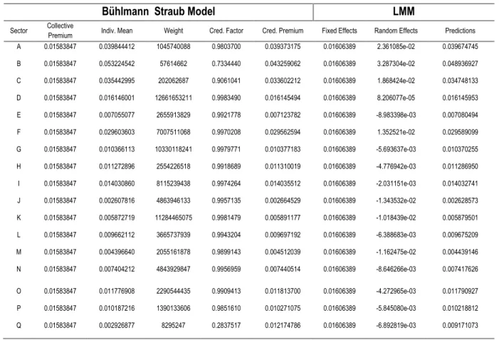
2.3. Model application: BS model
Now, reinforced with the previous results we will replicate the procedure from 2.1 to the BS model.
The formalization of the LMM will be quite similar:
(8) 𝑅𝑎𝑡𝑖𝑜𝑖𝑡 = 𝛽 + 𝑢𝑖 + 𝜀𝑖𝑡
with: 𝑢𝑖~𝑁(𝑂, 𝜎𝑢2) 𝑖. 𝑖. 𝑑 and 𝜀𝑖𝑡~𝑁(𝑂, 𝜎𝜀2/𝑤𝑖𝑡) 𝑖. 𝑖. 𝑑. As we can see the only improvement is the inclusion of the weights.
3 Which aren´t problematic, for instance, Klugmam (2014) reminds that: “While we may not believe that
the normal distribution is the correct model, we do note that there is a correspondence between the normal distribution and least squares estimation”.
P á g i n a 18 | 46
Before we get model application, we would like to present a more articulated theoretical evidence
sustaining the closeness between both concepts. Unfortunately, the limitations of space doesn´t
allow us to be as extensive as we wish in this approach. Nevertheless, we present in Annex 2, an
analytical demonstration of the equivalency between the presented LMM and the BS model under
some assumptions.
Returning to the model application, the results obtained this time will need a more attentive
interpretation:
Unlike with the Bühlmann model, we didn´t get an absolute coincidence of results, although they
weren´t generally that far. This results are consistent with the similar approach applied by Antonio
and Zhang (2014a) to the Hachemeister data; the authors relate the non-absolute equality in the
results with differences in the methods of estimation (Method of moments in the credibility
calculations; restricted maximum likelihood (REML) in the software package that we are using in
Bühlmann Straub Model LMM
Sector Collective
Premium Indiv. Mean Weight Cred. Factor Cred. Premium Fixed Effects Random Effects Predictions A 0.01583847 0.039844412 1045740088 0.9803700 0.039373175 0.01606389 2.361085e-02 0.039674745
B 0.01583847 0.053224542 57614662 0.7334440 0.043259062 0.01606389 3.287304e-02 0.048936927
C 0.01583847 0.035442995 202062687 0.9061041 0.033602212 0.01606389 1.868424e-02 0.034748133
D 0.01583847 0.016146001 12661653211 0.9983490 0.016145494 0.01606389 8.206077e-05 0.016145953
E 0.01583847 0.007055077 2655913829 0.9921778 0.007123782 0.01606389 -8.983398e-03 0.007080494
F 0.01583847 0.029603603 7007511068 0.9970208 0.029562594 0.01606389 1.352521e-02 0.029589099
G 0.01583847 0.010366113 10330118241 0.9979771 0.010377183 0.01606389 -5.693637e-03 0.010370255
H 0.01583847 0.011272896 2554226518 0.9918689 0.011310019 0.01606389 -4.776942e-03 0.011286950
I 0.01583847 0.014030860 8115239438 0.9974264 0.014035512 0.01606389 -2.031151e-03 0.014032741
J 0.01583847 0.002607816 4863946133 0.9957135 0.002664529 0.01606389 -1.343532e-02 0.002628573
K 0.01583847 0.005872719 11284465075 0.9981479 0.005891177 0.01606389 -1.018439e-02 0.005879501
L 0.01583847 0.009662112 3665737939 0.9943204 0.009697192 0.01606389 -6.388683e-03 0.009675209
M 0.01583847 0.004396640 2055161878 0.9899143 0.004512039 0.01606389 -1.162475e-02 0.004439146
N 0.01583847 0.007404212 4843929847 0.9956959 0.007440514 0.01606389 -8.646266e-03 0.007417626
O 0.01583847 0.011776908 2290544435 0.9909413 0.011813700 0.01606389 -4.272965e-03 0.011790927
P 0.01583847 0.010187216 1390133606 0.9851610 0.010271075 0.01606389 -5.845080e-03 0.010218812
Q 0.01583847 0.002926877 8295247 0.2837517 0.012174786 0.01606389 -6.892819e-03 0.009171073
P á g i n a 19 | 46
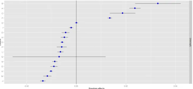
this chapter). Also, Klugman (2015) points a bias effect in REML estimates when the total
exposures differ among groups, but we believe that we should go deeper in this analysis. First,
let´s get a look to the graphical representation of the random effects in Figure 2.
We see that the biggest divergences in the predictions are related with the sectors with wider
prediction intervals, consequence of having an inferior weight (which, according with the model
specification, is inversely proportional to the variance). It´s important to point out that, even though
of the differences to the traditional application of the BS model, the implemented LMM stills very
effective in the inclusion of a shrinkage to the mean effect.
2.4. Model application: Hierarchical model. First level: CAE, Second level: Sector
To the next example following the same of reasoning, we can write a LMM functionally equivalent
to a hierarchical model by:
(9) 𝑅𝑎𝑡𝑖𝑜𝑘𝑖𝑡 = 𝛽0+ 𝛾𝑘+ 𝑢𝑘𝑖 + 𝜀𝑘𝑖𝑡
with:
𝛾𝑘~𝑁(𝑂, 𝜎𝛾2) 𝑖. 𝑖. 𝑑, 𝑢𝑖𝑘~𝑁(𝑂, 𝜎𝑢2) 𝑖. 𝑖. 𝑑 and 𝜀𝑘𝑖𝑡~𝑁(𝑂, 𝜎𝜀2/𝑤𝑖𝑡) 𝑖. 𝑖. 𝑑.
P á g i n a 20 | 46
We have repeated the same exercise as in the previous two model applications. Here we will need
an additional hierarchical level so we will use, again, the CAE. Figure 3 presents the differences
of the predictions coming from the traditional credibility hierarchical model and the LMM.
As we can see, generally we get quite coincident results, even thought that to around 5% of CAE´s
the differences are above 0.01. Although we didn´t see this kind of experience reproduced
anywhere else, we believe that the arguments presented by Antonio and Zhang (2014a) to the BS
model are even more relevant here, since the hierarchical model needs one supplementary
estimation of variance to the newly introduced level (actually, figure 3 suggests some sector specific
anomalies). We choose not reproduce the data here, it seems, nevertheless, to be a relation
between the differences in the predictions and the weights of each CAE, suggesting that there
could be a tendency to the mixed model be less severe in the shrinkage effect in the most sparsely
exposed CAE.
2.5. Some final relevant notes
One of our major sources of interest in the connection between classical credibility models and the
LMM framework was to find an intuitive, user friendly, tool to implement the credibility models, since
LMM are available in the basic menu of SAS, the software generally used for predictive tasks at
Fig. 3 - Differences in the predicted CAE premium between classical hierarchical model and the
P á g i n a 21 | 46
Fidelidade. Moreover, now we are allowed to use all the powerful analytical and graphical arsenal
of regression to evaluate the usefulness of several models (although we didn´t use those tools that
much in this particular work). Also, the variety of models at our disposal increases significantly; for
instance, crossed effects models, which evolve a relatively complex process of estimation, could
be implemented using this path. We think that it was sufficiently stated that the approximations
between both models could enrich largely the practice of credibility evaluation. What about the
reverse direction? Can credibility help to solve some difficulties of the regression models when
dealing with real world data? We believe so and our final chapter will try to exemplify how.
3. Credibility and generalized linear mixed models
Linear models aren´t, as far as we know, a major tool in actuarial practice, since the normality
assumptions doesn´t seem to fit the most frequent data sets used in the insurance industry. The
road taken by regression modelling in this field is the generalized linear modelling. GLM became
probably the most powerful resource of the actuaries in the so called, a priori risk classification:
selecting and measuring the most significant risk factors of a particular portfolio. It isn´t hard to
understand why: there are several very intuitive software packages able to apply this approach;
also the GLM´s outputs are easy to interpret and improve, an enormous advantage in commercial
world. However that doesn´t imply the obsoleteness of the credibility models; they still have an
important role, given their ability to capture individual specific behaviours that couldn´t be traced by
the GLM a priori approach. The results presented in Chapter 2, however, suggests a question: can
we do better? Since we were able to include the credibility in the linear models, could we do the
same with their generalized form? As the famous struggle of modern physics, can we find a unified
P á g i n a 22 | 46
3.1. From GLM to GLMM´s
GLM is a regression model where the response variables 𝑦𝑖 are assumed to be independent and
have a probability distribution that can be written as:
(10) 𝑓𝑦(𝑦) = 𝑒𝑥𝑝 (𝑦𝜃 − 𝜓(𝜃)𝜙 + 𝑐(𝑦, 𝜙))
which defines the so called exponential dispersion family. There are several useful properties
associated with these kinds of distributions; for instance, it can be easily shown that the mean and
variance are related, since:
(11) 𝑢 = 𝐸(𝑦) = 𝜓′(𝜃) and 𝑉𝑎𝑟(𝑦) = 𝜙 𝜓′′(𝜃)= 𝜙𝑉(𝑢).
Within this type of regression, the predictor variables 𝑥𝑖𝑗 are combined into linear predictors:
(12) 𝜂𝑖 = 𝛽0+ 𝛽1𝑥𝑖1+ ⋯ + 𝛽𝑘𝑥𝑖𝑘
where the coefficients 𝛽0, 𝛽1, 𝛽𝑘 are estimated using maxing likelihood estimation. Finally, the
expected values of 𝑦𝑖 -𝜇𝑖- are predicted using the inverse function of a monotonic and differentiable
link function 𝑔(𝑥).
Similarly to the LMM extension of the ordinary linear models, the GLMM´s add a random effect 𝑊𝑢
to the right side of (12). According to Antonio and Zhang (2014b), those random effects would
enable cluster-specific analysis and predictions. More formally, and conditionally on a
q-dimensional vector 𝑢𝑖, we can summarize the GLMM´s assumptions for the jth response on cluster
or subject i,
𝑦𝑖𝑗|𝑢𝑖~𝑓𝑌𝑖𝑗|𝑢𝑖(𝑦𝑖𝑗|𝑢𝑖)
𝑓𝑌𝑖𝑗|𝑢𝑖(𝑦𝑖𝑗|𝑢𝑖) = 𝑒𝑥𝑝 (
𝑦𝑖𝑗𝜃𝑖𝑗 − 𝜓(𝜃𝑖𝑗)
𝜙 + 𝑐(𝑦𝑖𝑗, 𝜙)).
Where 𝑢𝑖 are independent among clusters 𝑢𝑖, with a distributional assumption: 𝑢𝑖~𝑓𝑈(𝑢𝑖). In our
model applications we will use normally distributed random effects, although other assumptions are
admissible. Analogous to (11), the following conditional relations also hold:
P á g i n a 23 | 46
3.2. Model application: 2014 losses
We should have reasonable expectations that GLMM´s could also generalize the link between
credibility and LMM. We will start with a simple example, which should shed some light to how the
credibility (via GLMM´s) could improve the customary actuarial practice with GLM´s.
The idea could be found for instance in Guszcza (2011) (and, although in a seemingly different
shape, in Ohlsson and Johansson (2010)) and answers a familiar question to those usually
engaged with the actuarial practice using GLM. Frequently we find in our models some sparsely
populated levels (in Guszcza example: some body types of vehicles), with a high estimate but also
low statistical significance, due to their reduced exposure. How should we deal with them? The size
of parameter tell us that there could be some relevant effect there, whereas the low value of
significance acts like a warning about the real extension of that effect; should we discard that
estimate and use instead the mean? Should we use the GLM estimate ignoring the information
about the significance?
The GLMM approach could increase our range of choices. Ideally, the random effect will gave a
shrunken to the mean effect, so acts like a credibility weighted compromise between the two
solutions proposed above; in other words, we expect that the GLMM estimates to the sparsely
exposed levels will be prudently close to the mean while the levels highly exposed will have a
GLMM relativity close to the relativity suggested by a GLM.
To testify that process we have tried to replicate with our data set a case study presented in Klinker
(2011). We used three categorical variables with relevance in the ratemaking process: one related
with the dimension of the company, another with the area where the company is located and a third
one with the CAE. The first two were treated like fixed effects, our comparisons will have the CAE
as target.
The design of this experience is simple and, in our view, quite ingenious. Our response variable
will be the ratio between losses and the premium in 2014 (usually known by loss ratio). The idea is
P á g i n a 24 | 46
same exercise with a GLMM were the CAE´s will be treated as random effects. Finally, comparing
the results, we will try to detect some evidence of shrinkage to the mean effect related with the
volume of the exposure - the volume is introduced in the model by means of weights specification.
We have used the increasing popular Tweedie distribution with link function log. In our approach,
the Tweedie distribution will behave like a compound Poisson with a Gamma as secondary
distribution. This model as two main advantages; first: it deals simultaneously with the number and
extension of each claim. Also, it is reported as being particularly well fitted to describe data sets
implying a distribution with an important mass point at 0 and very skewed continuous data, features
obviously desirable in the workers compensation framework. It can also be pointed, as many
authors did, that a sequential approach, modelling first the claims and after the severity, is more
adequate, since it allows an enlarged insight of the several components within the losses. As our
proposes are demonstrative, we can disregard this argument (more: there are several reports
claiming difficulties in the implementation of the Gamma distribution within the GLMM´s
computation). For a similar reason we were not extremely careful in the process of search the best
parameter p. We have used the same value as Klinker (2011) (p=1.67) since it appears to be a
popular choice for this kind of data. Some preliminary notes should be made: in this model
application we have only used the policies in force during 2014, due missingness in data the GLM
procedure have deleted additionally around 3500 observations (and incidentally three whole
CAEs). The results for the first twenty CAEs are summarized in the table below.
CAE (1) Weights (2) Fixed E. (3) exp(FE) (4) Relativity F. (5) Random E. (6) exp(RE) (7) Relativity R. (8) IC (9)
11 62490930 0.0000 1.0000 1.2817 0.2486 1.2822 1.2653 0.9417
12 15860310 0.4441 1.5590 1.9982 0.5702 1.7685 1.7453 0.7466
13 7166521 0.2247 1.2520 1.6047 0.3062 1.3582 1.3404 0.5628
14 20608450 -0.1166 0.8899 1.1407 0.1206 1.1282 1.1134 0.8059
15 404375 0.7903 2.2041 2.8251 0.1228 1.1307 1.1158 0.0635
20 14488000 0.0661 1.0683 1.3693 0.2539 1.2891 1.2721 0.7369
50 10283410 0.4366 1.5475 1.9835 0.5156 1.6746 1.6525 0.6635
Table VI - Results from the application of Klinker (2010) experience in our portefolio (extract). Note
P á g i n a 25 | 46
131 16200 -0.5744 0.5630 0.7216 -0.0008 0.9992 0.9861 0.0501
132 10200000 -0.6144 0.5410 0.6934 -0.2373 0.7888 0.7784 0.7227
141 4956633 -0.4483 0.6387 0.8186 -0.0878 0.9160 0.9039 0.5298
142 5168791 -0.5800 0.5599 0.7176 -0.1508 0.8600 0.8487 0.5357
143 17654 -1.1496 0.3168 0.4060 -0.0020 0.9980 0.9849 0.0254
144 472729 -0.1531 0.8580 1.0997 0.0103 1.0104 0.9971 -0.0291
145 849632 -0.7800 0.4584 0.5875 -0.0623 0.9396 0.9273 0.1764
151 23743400 -0.1200 0.8869 1.1368 0.1246 1.1327 1.1178 0.8610
152 2886682 -0.4052 0.6668 0.8547 -0.0535 0.9479 0.9354 0.4444
153 4736808 0.0486 1.0498 1.3456 0.1672 1.1820 1.1664 0.4816
154 12309420 -0.0559 0.9456 1.2120 0.1622 1.1761 1.1606 0.7575
155 12016320 0.0177 1.0179 1.3046 0.2111 1.2350 1.2187 0.7181
156 2864224 -0.6124 0.5421 0.6948 -0.1196 0.8873 0.8756 0.4076
In column 2 are the values of the capital exposure by each CAE in 2014. Column 3 includes the
coefficients estimated by the GLM model, while in column 6 are the random effects obtained using
a GLMM. Now, as our idea is to compare both effects, we need some few adjustments in those
values in order to get a fair balance between those estimates. For instance, in the GLM the
coefficients for each CAE were obtained by their relative effect regarding a base level, determined,
in this case, by the CAE 11 ( in the GLMM such procedure is not applied).
So, in order to do our comparisons, we will start to revert the effect of the link function applying the
exponential function to the coefficients presented in 3 and 6; the results are in column 4 and 7.
Next, we followed a suggestion by Klinker (2010), we will “normalize” both effects, so they can be expressed relative to base level of mean one (column 5 and 8). The idea is to divide each one of
exponentials in column 4 and 7 by their column weighted mean, in order to take in account the
weighted specifications of our generalized models. After that, we should be able to make
reasonably comparisons between both effects. We can see that, with one exception (to which we
will return), the random relativities, suggested by the GLMM, shrunk to one the fixed relativities
obtained with the GLM. Also, as we can see Figure 4, the dimension of that shrinking seems to be
P á g i n a 26 | 46
Finally, we can measure the shrinking to the mean effect, defining an Inferred Credibility (IC) by:
(13) IC =(column(5) − 1)(colum (8) − 1)
obtaining the column 9.
The results obtained with our data didn´t seem as categorical as those reported by Klinker (2011),
for instance: around 8% of our IC´s is located outside the critical boundary [0,1] (e.g: CAE 144
included in table IV). However, they aren´t either as disappointing as a premature look may
suggest, since the original experience that we try to replicate also have issues with the boundary
[0,1] - in that case were analysed the results of twelve classes, one of them outside the desired
interval, so not far from our percentage. Two possible explanations for those circumstances were
suggested: first, when the levels of relativities are very close to one (which is usually the case of
our problematic IC´s), the implementation of (13) becomes very vulnerable even to small distortions
in the results; small differences in the level of the second or third decimal place could have
important impacts in the result. Also, it is suggested that the process that leads to the calculation
of the values in column 6 and 8 could introduce some correlations among the parameters. We
could add an argument explained in Antonio and Zhang (2014b). Both Klinker´s and our experience
have implement the GLMM using the Pseudo-likelihood algorithm, this procedure isn´t in general
2.5
2.0
1.5
1.0
Fig. 4– Relativities obtained with the GLM and GLMM for the first ten CAE´s and their relation with
P á g i n a 27 | 46
the most accurate way of implement the GLMM´s, although in other hand it is, by far, the most
flexible - we weren´t, for instance, able to apply other methods to this particular problem.
It should be pointed, either way, that the IC outside the boundary in the original experience was
anyhow pretty close (1.05) the upper level, while we got values as extreme as 4.34. Getting our
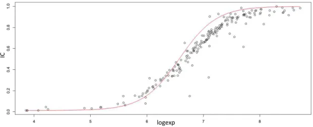
attention to values inside the boundary, nevertheless, we could try to find evidences for credibility.
For instance, we could plot the values of the IC´s for each one of those CAE´s and see if there is
relation between those values and the exposure of CAE: in order words to check if, as we expected
from the credibility theory, larger CAEs have bigger IC´s and the reverse for the smaller ones. We
can go even further: stating that
ICi = 𝑊 𝑊𝑖 𝑖+ 𝐾i ,
we get two hundred and ten different, although generally close, values for 𝐾𝑖. Let´s choose, for
instance, the median of those values 𝐾𝑚; we can also check if the theoretical credibility suggested
by function y=x/(x+𝐾𝑚) (represented in red in Figure 5) relates somehow with the pattern observed
in the plot with the values of IC´s.
The results obtained, although not immaculate (especially if we remember that around 8% of the
CAEs were not included in the plot), are in our view convincing enough to state that, at least to
some degree, the link between credibility and linear mixed models isn´t completely lost with the
generalization of the formers.
Fig. 5 - Relation between inferred credibility and the common logarithm of exposures.
IC
P á g i n a 28 | 46
3.3. Model application: forecasting the number of claims
Finally, we have tried to use those techniques in a predictive task. We were confident that the
introduction of random effects could allowed us to build a model capable to cope a priori and a
posterior ratemaking to every policy. Unfortunately, we were soon confronted with several
computational issues, the available implementations of the GLMM´s algorithms, when applied to a
larger set of data, demands an amount of hardware resources that we weren´t able to fulfil. After
several frustrating attempts, it became clear that this approach could only be applied to small
subsets of our data.
We decided instead to try another direction; our inspiration came from the Chapter 4 of Ohlsson
and Johansson (2010). In this work it is described a credibility-enhanced method of application of the GLM´s. Roughly, the idea formulated in this text is to use classical Bühlmann-Straub reasoning
in order to improve the reliability of GLM´s estimates related with scarcely populated level. We find
this problem somehow reminiscent of the GLMM´s applications prescribed by Guszcza (2011) and
Klinker (2011); so we´ve wonder if this approach could also be useful in the problem we´ve
struggled to solve with the GLMM´s software implementations. As we will see, the results collected
were encouraging.
The general framework followed is quite simple. The authors considered a multiplicative tariff:
(14) 𝐸[𝑋𝑖𝑡|𝐼𝑖] = 𝑢 𝛾𝑖1 𝛾𝑖 2… 𝛾𝑖𝑛𝐼𝑖 .
𝑋𝑖𝑡 is again our key ratio, 𝛾𝑗𝑖 (𝑗 = 1, … 𝑛) represents a priori ratemaking factors like geographical
zone or sector of activity that could be estimated using GLM´s. Similarly, 𝑢 will play the role of the
intercept term of the GLM estimation. 𝐼𝑖 will be treated as a random effect and estimated using
credibility. In Ohlsson and Johansson (2010) text, 𝐼 denotes a problematic ratemaking variable,
while our interpretation associates 𝐼𝑖 with the individual features, unrelated with the a priori
ratemaking factors, of policy 𝑖.
We will assume, in order to avoid redundancy between the parameters, that E(𝐼𝑖) = 1. We will
P á g i n a 29 | 46
with this procedure we can stablish a correspondence between this new notation and the one
presented in the first chapter: 𝑉𝑖 will have a similar role to 𝑢(𝜃𝑖). As a consequence:
(15) 𝐸[𝑋𝑖𝑡|𝑉𝑖] = 𝛾𝑖1 𝛾𝑖 2… 𝛾𝑖𝑛 𝑉𝑖.
For sake of simplicity we will also represent the fixed effects 𝛾𝑖1 𝛾𝑖 2… 𝛾𝑖𝑛 just with 𝛾𝑖 . Further
steps will renounce to some generality of the framework, as they are only valid for Tweedie models.
Luckily, this kind of models are the standard practice in ratemaking modelling. Working with these
distributions it is known (see Ohlsson and Johansson (2010) for details) that:
(16) 𝑉𝑎𝑟[𝑋𝑖𝑡|𝑉𝑖] = 𝜙( 𝛾𝑖 𝑉𝑖)𝑝/𝑤𝑖𝑡 .
Also, if we take 𝜎2 = 𝜙𝐸[𝑉𝑖𝑝] , we can write:
(17) 𝐸[𝑉𝑎𝑟[𝑋𝑖𝑡|𝑉𝑖]] =𝛾𝑖 𝑝𝜎2
𝑤𝑖𝑡 .
In order to make our reasoning more clear, we will rewrite the BS assumptions of our first chapter
in an equivalent, Ohlsson and Johansson (2010) fashion way:
BSO1- The random vectors (𝑋̃ , 𝑉𝑖𝑡 𝑖), i =1,2,….J; are independent.
BSO2- The 𝑉𝑖 i =1,2,….J are identically distributed with 𝐸[𝑉𝑖] = 𝑢 > 0 and 𝑉𝑎𝑟[𝑉𝑖] = 𝑎 > 0.
BSO3- Conditional on 𝑉𝑖 the vector of realizations 𝑋̅ = (𝑋𝑖 𝑖1, 𝑋𝑖2,… , 𝑋𝑖𝑇𝑖), 𝑖 = 1,2, … 𝑇 are
mutually independent with mean 𝐸[𝑋̃ |𝑉𝑖𝑡 𝑖] = 𝑉𝑖 and 𝐸 [𝑉𝑎𝑟[𝑋̃ |𝑉𝑖𝑡 𝑖]] = 𝜎2
𝑤̃𝑖𝑡 .
To fulfil those guarantees we need a subtle transformation of the observations. Considering:
𝑋̃ = 𝑋𝑖𝑡 𝛾𝑖𝑡
𝑖 𝑎𝑛𝑑 𝑤̃ = 𝑤𝑖𝑡 𝑖𝑡𝛾𝑖 2−𝑝
we have not only that:
𝐸[𝑋̃ |𝑉𝑖𝑡 𝑖] =𝛾1
𝑖𝐸[𝑋𝑖𝑡|𝑉𝑖] = 𝑉𝑖
using (15), but also,
𝐸 [𝑉𝑎𝑟[𝑋̃ |𝑉𝑖𝑡 𝑖]] =𝛾1
𝑖2𝐸[𝑉𝑎𝑟[𝑋𝑖𝑡|𝑉𝑖]] =
1 𝛾𝑖2
𝛾𝑖𝑝𝜎2
𝑤𝑖𝑡 =
𝜎2