José Rodrigo Ferreira Baleia
Licenciado em Ciências da Engenharia Eletrotécnica e de
Computadores
Haptic Robot
-
Environment Interaction
for Self
-
Supervised Learning in Ground
Mobility
Dissertação para obtenção do Grau de Mestre em
Engenharia Eletrotécnica e de Computadores
Orientador: Prof. Doutor José António Barata de Oliveira,
FCT-UNL
Co-orientador: Prof. Doutor Pedro Figueiredo Santana,
ISCTE-IUL
Júri:
Presidente: Doutor Ricardo Luís Rosa Jardim Gonçalves – FCT-UNL Arguente: Doutor Pedro Alexandre da Costa Sousa – FCT-UNL
Copyright
Haptic Robot-Environment Interaction for Self-Supervised Learning in
Ground Mobility
A Faculdade de Ciências e Tecnologia e a Universidade Nova de Lisboa têm o direito, perpétuo e sem limites geográficos, de arquivar e publicar esta dissertação através de exemplares impressos reproduzidos em papel ou de forma digital, ou por qualguer outro meio conhecido ou que venha a ser inventado, e de a divulgar através de repositórios científicos e de admitir a sua cópia e distribuição com objectivos educacionais ou de investigação, não comerciais, desde que seja dado crédito ao autor e editor.
Acknowledgements
I would like to thank my thesis supervisor Prof. Jose Barata for his support and for giving me the opportunity and enabling the resources for the hardware necessary for the robot implementation. I would also like to thank other professors from the institution, whose teachings had a big role in my growth not only as an engineering student but also a human being.
A special note of gratitude to my co-supervisor Prof. Pedro Santana, whose vision and knowledge on the field of robotics motivated and inspired me to accomplish more as an engineer. I’m grateful for the constant inputs on the overall work and readiness to help and improve. I would also like to thank Eduardo Pinto, whose hardware expertise were essential for the development of the robot.
My next acknowledgments go to all the ones whose paths crossed mine in this long journey of becoming an electrical engineer. A special word of thanks to Gustavo Fradique, Nuno Barata, Fernando Costa, Pedro Carvalho, Rui Borrego, Pedro Barreira, André Pereira, João Patrício, João Silva, and many others, that started out as colleagues and ended up as friends. I would also like to thank my work colleague Pedro Alves for his support in the roughness that is field testing.
Abstract
This dissertation presents a system for haptic interaction and self-supervised learning mecha-nisms to ascertain navigation affordances from depth cues. A simple pan-tilt telescopic arm and a structured light sensor, both fitted to the robot’s body frame, provide the required haptic and depth sensory feedback. The system aims at incrementally develop the ability to assess the cost of navi-gating in natural environments. For this purpose the robot learns a mapping between the appearance of objects, given sensory data provided by the sensor, and their bendability, perceived by the pan-tilt telescopic arm. The object descriptor, representing the object in memory and used for comparisons with other objects, is rich for a robust comparison and simple enough to allow for fast computations. The output of the memory learning mechanism allied with the haptic interaction point evaluation prioritize interaction points to increase the confidence on the interaction and correctly identifying ob-stacles, reducing the risk of the robot getting stuck or damaged. If the system concludes that the object is traversable, the environment change detection system allows the robot to overcome it. A set of field trials show the ability of the robot to progressively learn which elements of environment are traversable.
Resumo
Esta dissertação apresenta um sistema para interação háptica e mecanismos de aprendizagem auto-supervisionada para averiguar as possíveis ações sobre objetos a partir de informação sen-sorial. Um braço telescópico para obter informação háptica e um sensor de profundidade baseado na projeção de luz estruturada, ambos incluídos no chassis do robô, fornecem os requisitos para a geração de metodologias de interação háptica. O objetivo do sistema é o de continuamente avaliar o custo de navegação em ambientes naturais. Para alcançar este objetivo, o robô aprende o mapea-mento entre a aparência dos objetos, dada a informação sensorial, e a sua rigidez, percecionada através do braço telescópico. O descritor do objeto, representação do objeto em memória e utilizado para a comparação com outros objetos, é rico para permitir uma comparação robusta e simples para ser de rápida computação. O resultado do mecanismo de aprendizagem aliado com a análise ge-ométrica do objeto prioriza pontos de análise para aumentar a confiança na interação e corretamente detetar obstáculos, reduzindo o risco do robô ficar preso ou danificado. Se o sistema conclui que o objeto é trespassável, o sistema de deteção de mudança de ambiente permite ao robô atravessá-lo. Um conjunto de testes no terreno demonstra a capacidade do robô de aprender progressivamente que elementos do ambiente são trespassáveis.
Contents
List of Figures xv
List of Tables xvii
1 Introduction 1
1.1 Dissertation Outline . . . 3
2 Related Work 5 2.1 Interaction Methods . . . 5
2.2 Haptic-visual relation . . . 7
2.3 Vegetation Characterization . . . 7
2.4 Affordances . . . 9
2.5 Traversability . . . 10
2.6 Self-Supervised Learning . . . 12
3 Supporting Concepts 15 3.1 Point Clouds . . . 15
3.2 Random Sample Consensus (RANSAC) . . . 16
3.3 Voxel Grid . . . 17
3.4 Histograms . . . 18
3.5 Octree . . . 19
3.6 Supporting tools . . . 19
3.6.1 Robot Operating System (ROS) . . . 20
3.6.2 Point Cloud Library (PCL) . . . 21
4.2 Model Overview . . . 23
4.3 Calibration . . . 26
4.4 Object Evaluation . . . 28
4.4.1 Learning from Memory Evaluation . . . 28
4.4.1.1 Object Descriptor . . . 28
4.4.1.2 Memory Recall . . . 32
4.4.2 Interaction Points Evaluation . . . 34
4.4.3 Interaction with the Object . . . 38
4.5 Environment Change Detection . . . 41
5 Prototype 43 5.1 Prototype Overview . . . 43
5.2 Telescopic Antenna . . . 45
5.3 Depth Sensor . . . 47
5.4 Mobile platform . . . 48
6 Experimental results 51 6.1 Model Parametrization . . . 51
6.1.1 Calibration Parameters . . . 51
6.1.2 Object Evaluation Parameters . . . 53
6.1.3 Interaction and Environment Crossing Parameters . . . 54
6.2 Test results . . . 54
6.2.1 Classification Accuracy from Haptic Interactions . . . 55
6.2.2 Classification Accuracy from Learning . . . 56
6.2.2.1 Object Recognition . . . 59
6.2.2.2 Object Generalization . . . 59
6.2.2.3 Impact of alpha on the system interaction and speed . . . 61
6.2.3 Environment Change Detection . . . 61
7 Conclusions and Future Work 65 7.1 Conclusions . . . 65
7.2 Future Work . . . 66
List of Figures
2.1 Coordinate systems of the vibrissal system . . . 6
3.1 A point cloud image of a torus. . . 16
3.2 Voxel representations. The image on the left represents a single voxel, while the middle represents a voxel set. The image on the right shows a voxel grid. (Zirbes, 2014) . . . 18
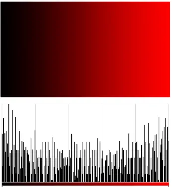
3.3 Example of a bar histogram representing the distribution of intensity levels for the red channel. . . 18
3.4 Space discretization of a cube and the corresponding octree depth. (Ferrando et al., 2011) . . . 19
3.5 ROS service communication between nodes diagram (adapted from ROSWiki (2014)). 21 4.1 Front and side view of the robot model. . . 24
4.2 Proposed system’s major steps. . . 24
4.3 Proposed system’s workflow. . . 25
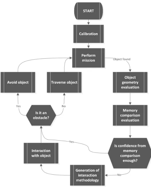
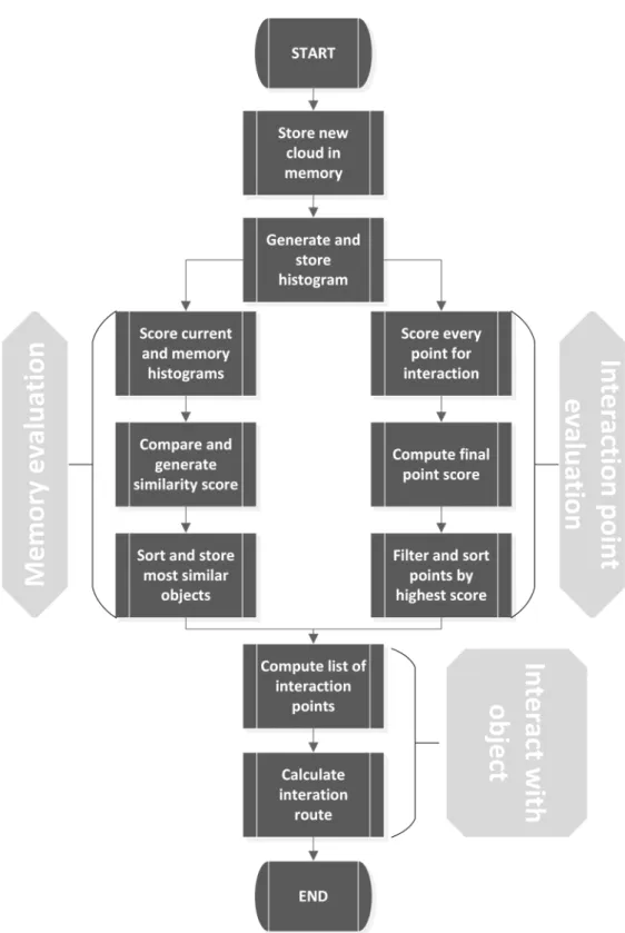
4.4 Flowchart showing both evaluations and interaction process. . . 29
4.5 Grid of dimensionsxH= 8 andyH= 10 being applied to a cloud. . . 30
4.6 Perspective view of the cloud where the histogram grid was applied. . . 31
4.7 Change of inclination impact on theyaxis. . . 31
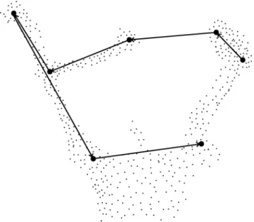
4.8 Example of a line evaluated by the described method. . . 32
4.9 Example of the sorting algorithm filter being applied. . . 37
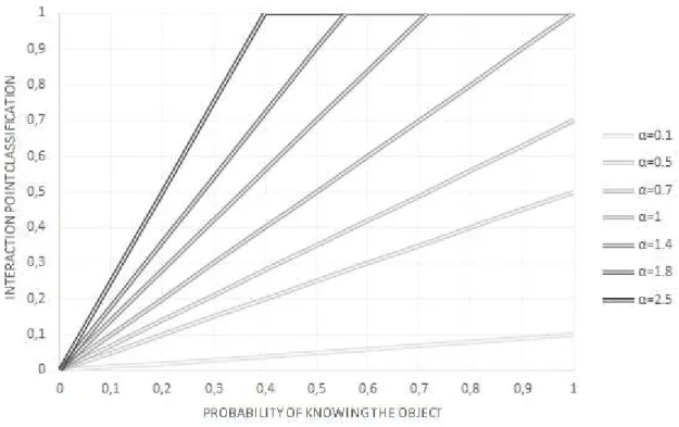
4.10 Effect ofαon the confidence of the system. . . 39
4.11 Example of a cloud being swept after evaluation. . . 40
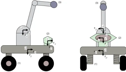
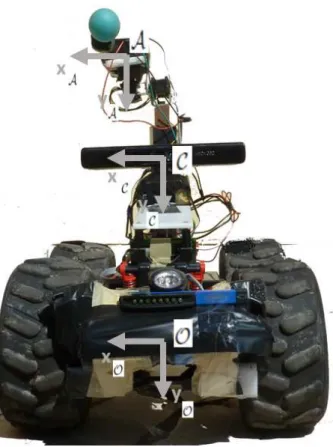
5.1 Front prototype view with the associated frames of reference. . . 44
5.2 Side prototype view with the associated frames of reference. . . 44
5.3 Layers and communications of the experimental setup. . . 45
5.5 Installation schematics of the phototransistor and encoder used. . . 47
5.6 Detail of the phototransistor and the encoder setup in the prototype system. . . 47
5.7 Robotic arm coordinate schematic. . . 48
5.8 Microcontrollers location and connections. . . 48
5.9 The robot prototype with its arm stretched to its maximum range. . . 49
6.1 Time lapse image of the calibration procedure. . . 52
6.2 Scoring system based on 3 tiers . . . 54
6.3 Objects used for classification accuracy analysis in a controlled environment (data set 1). . . 55
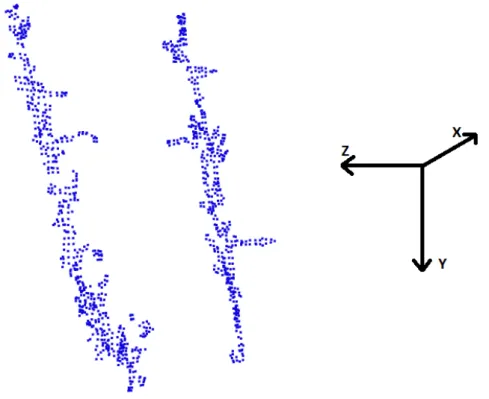
6.4 Object point clouds captured. . . 56
6.5 Typical haptic interaction execution. . . 57
6.6 Different interaction points suggested by the system for two objects. . . 57
6.7 First object used for the memory evaluation test (). . . 58
6.8 Second object used for the memory evaluation test (). . . 58
6.9 Classification confidence when progressively incorporating two new objects into memory. 59 6.10 Results on the random introduction to memory test. . . 60
6.11 Confusion matrix obtained from leave-one-out cross-validation. . . 60
6.12 Impact of differentαon the number of interactions. . . 62
6.13 Traversability test subjects. . . 63
List of Tables
6.1 Coordinates used for calibration, from the arm reference axisA. . . 52
6.2 Number of points selected for haptic interaction within a given score interval. . . 56
6.3 Classification of objects in data set 1 given knowledge about objects in data set 2 with k= 5. . . 61
6.4 Confidence levels and systems guess between same object encounters. . . 61
6.5 Results for traversing object (a) to open environment. . . 62
6.6 Results for traversing object (a) to closed environment. . . 63
6.7 Results for traversing object (b). . . 64
List of Notations
α Memory confidence factor
αC Weight of parameterCh(P)
αS Weight of parameterNHj(H’)
αρ Environment change difference threshold
βC Weight of parameterCd(P)
βS Weight of parameterWHj(H’)
∆ρ Relation betweenρjHandρ
j
H’
∆P Relation betweenPHjandP
j
H’ δS Weight of parameterPHj(H’) δρ Environment change difference
γC Weight of parameterCρ(P)
γS Weight of parameterρjH(H’)
A Robot Arm frame of reference
C Sensor frame of reference
H Histogram formalization
O Base of the robot frame of reference
µ Distance from sensor to wheel height
ω Comparison factor forWHj(H’)score
ρjH(H’) Comparison ofρjHscore between histogramH’andH
ρjH Point density per linejin histogramH
σ Robot architecture and sensor adaptive factor
τ Distance to the sensor dependence factor
c Coordinates to which the point is found in theCandAframe of reference
S List of thenclosest neighbors by similarity
υ Comparison factor forNHj(H’)score
ζ Centroid of a point cloud
Cd(P) Distance to centroid score for point interaction
Ch(P) Height score for point interaction
Ck Confidence of knowing a new object from memory evaluation
CT(P) Final score for point interaction
CA Point in theAframe of reference
CC Point in theCframe of reference
Cρ(P) Number of neighbor points score for point interaction
Cint Cloud used to generate the interaction points
Clf Cloud with the background removed
Cln New captured cloud
Clbkg Cloud without robotic arm in range
Eo Object labeled as obstacle
Et Object labeled as traversable
F Furthest point in a cloud from the robots arm referential
Hf Filtered cloud used for histogram creation
Hv Voxelization of the filtered cloud
i Histogram column iterator
j Histogram line iterator
jo Number of bins occupied in a line
M CtoAtransformation matrix
M−1 InverseM matrix,AtoCtransformation matrix
Mnn Maximum number of points in a sphere
NHj(H’) Comparison ofNHj score between histogramH’andH
Nl Number of points in a line
np Number of points used for calibration
NHj Number of clusters per linejin histogramH
nc Number ofcfound
Pρ Relation betweenPHjandP
j
H’
PHj(H’) Comparison ofPHjscore between histogramH’andH
Po Probability of the object being an obstacle
Pt Probability of the object being traversable
Pρ Density change input cloud value
PHj Maximum points in a cluster per linejin histogramH
P sρ Density change first input cloud value
R Rightmost point from the arm
rint Robot end effector interaction radius
rn Neighbor points search radius
SHj(H’) Score from comparing a single line between two a histogramHandH’
Scl Size of the input cloud
Svox Size of the cloud after voxelization
To Traversability of a object in memory
WHj(H’) Comparison ofWHjscore between histogramH’andH
WHj Largest cluster per linejin histogramH
xH Number of columns in a histogram
yH Number of lines in a histogram
SH′
H Similarity score between two histogramsHandH’
P Point in a x, y, z coordinate system
Chapter 1
Introduction
Since the first invertebrate ventured out of the Panthalassa, the ability to navigate through the environment became crucial for the species survival. Nature evolved in order to allow for different means of interaction and learning mechanisms, some insects developed antennas to sense the sur-roundings, while mammals brains grew to support the big influx of information provided by non-haptic feedback, like hearing, vision and olfactory perception.
Inspired by Nature, in which visual and haptic sensory feedback are known to be jointly exploited in the Human brain (Lacey et al., 2010; Schwenkler, 2013) this thesis presents an haptic robot-environment interaction system for self-supervised learning of vision skills for safe navigation. For this purpose, the robot is provided with a mechanism to learn a mapping between the volumetric appearance of obstacles, given sensory data provided by a depth sensor, and their bendability, per-ceived by physically interacting with them with a small arm. As interactions unfold, the robot grows its ability to properly assess the cost of navigating the environment from its depth sensor and, conse-quently, reducing the need for physical interactions. As a consequence, the robot’s spatial reasoning look-ahead grows significantly, which is key to ensure a safe navigation.
Models like Kim and Möller (2007) and Wijaya and Russell (2002) aim to mimic the simplicity and low processing power necessary to navigate the environment as used by some invertebrate species, like ants, or small mammals, like rats. On the other hand, some models went for a different route and created more complex interaction methods, aiming to give a deeper insight provided by interaction. An example of that is the model developed by Edsinger-Gonzales (2005), which recreated a complex hand which can sense force, or the model of Shin et al. (2010), recreating a force sensing arm. To learn how the species interact with the world is crucial to learn about the perception they have of the environment.
Chapter 1. Introduction
reaction to the interaction and use that experience to learn about its traversability. This non-invasive method offers safer results for the environment and to the subject under test, a desirable quality for field robots. U˘gur and ¸Sahin (2010) considered learning affordances from full-body interactions by moving the robot against the objects. Conversely, the system developed in this thesis proposes assessing navigation cost with a robotic antenna, which reduces the robot’s risk of getting stuck or damaged as well as it allows for a finer analysis of the object.
While studying the aspect is important to decide the best interaction, remembering past efforts allows for a long term evolution in the quality of those interactions. Lower animals use a match between the input image and the stored images (Tanaka, 1993) so inspired by this, a comparison method for self-supervised learning applied to robotics improves the interaction dynamics in the long run. The aspect of the object and the result of that interaction allows to enhance the knowledge of the surrounding world, and by applying an object descriptor and a memory recall system, both an empir-ical and theoretempir-ical weight is given to the decision. With this, the speed of interaction, meaning the time it spends with each object, and its quality is expected to improve as more object data is collected.
To correctly identify the objects found in nature, a robust descriptor is needed. Vegetation is not the same all around the world so it is difficult to find methods of classification and biomass estimation, and as shown by Lu (2006), this an area with room for more research. Flora can vary by size, mass, color, shape and density, making the correct classification of similar types of environments a challenging task. A correct flora descriptor is important to be able to learn from previous experiences, so a good descriptor is necessary. The descriptor has to be broad enough to be able to work in every kind of environment but specific enough to be able to detect flora changes in the surroundings. While flora is present in field environment, other natural objects such as rocks, trunks or man made objects can still be found and have to be correctly described.
In a natural environment, the system may encounter vegetation or other types of objects, such as rocks. To assess the traversability, the system must create a 3D descriptor for comparison with its memory. The knowledge of the common vegetation is important to create the descriptor. When comparing to previous encounters, the system applies what it has learned in order to generate a haptic interaction methodology by taking into account not only what was learned but also the probable best interaction points to assess the bendability affordance based on the object’s structure. This interaction is more detailed if the confidence in the new object is low, or coarser if the confidence is higher. If after the interaction the system concludes that the bendability affordance is present in the object, it proceeds to overcome it.
1.1. Dissertation Outline
1.1
Dissertation Outline
This dissertation is organized as follows:
Chapter 2 reviews the state of the art in affordances, traversability, self-supervised learning, inter-action methods and vegetation characterization;
Chapter 3 presents the supporting concepts of this work, like software libraries used, voxel grids and histograms;
Chapter 4 describes a possible model for the existing problems and the methods used for imple-mentation;
Chapter 5 shows and explains the prototype developed for testing the proposed model. Both hard-ware and softhard-ware perspective are approached;
Chapter 6 presents the experimental results based on the model and prototype developed, as well as the testing parameters used;
Chapter 2
Related Work
This chapter includes a description of the state of the art in robotic interaction methods, including projects offering different perspectives on the subject, the state of the art of recognition methods mainly based on natural environments, projects and studies about affordances, studies and systems about traversability and finally an explanation of self-supervised learning, including the merits of this learning mechanism.
2.1
Interaction Methods
Robotics often take biological inspiration in order to create robots that mimic what happens in nature to solve complex problems (Pfeifer et al., 2007). In nature one can find various methods of interaction, from seemingly simple mechanisms, like whiskers, to more mechanically complex, such as an human arm. These topics are deeply studied and a big array of solutions is available.
In a complex perspective, in order to simulate a human arm, a system needs to emulate the fine balance between stiffness and force control. To achieve this it is necessary to understand the actua-tors available and assemblies used. A commonly used actuator is based in series elastic actuaactua-tors (Pratt and Williamson, 1995). These actuators place an elastic element between the output of the ac-tuator and the robotic link to limit the high-frequency impedance of the acac-tuator to the stiffness of the elastic coupling. To limit the low-frequency impedance a linear feedback system is implemented to regulate the output torque of the actuator-spring system. Therefore, the series elastic actuators pro-vide low impedance across the frequency spectrum (Zinn et al., 2004). These actuators are mainly developed to provide safe human-robot interaction, by finding a safe balance between torque and speed. Recently, a different approach has been used in order to reach the same goal. The new trend is the use of variable impedance actuators, to achieve safe, energy-efficient, and highly dynamic motion (Vanderborght et al., 2013).
Chapter 2. Related Work
Figure 2.1:Coordinate systems of the vibrissal system (Ahissar and Knutsen, 2008).
deeper study of its capabilities (Vincent, 1915). Rodents use their whiskers to detect and identify objects in their proximal three-dimensional space. Each whisker shaft is embedded in a follicle struc-ture and mechanoreceptors surrounding the shaft measure the deflection in all directions. Whisker behavior involves repetitive (periodic or non-periodic) forward (protraction) and backward (retraction) movements of the whiskers. Whisker movements are largely synchronous on one side, but often oc-cur with a phase-shift across the two sides of the snout. Whiskers are usually grouped in vertical and horizontal rows, and each row is used to sense different information about the surroundings (Ahissar and Knutsen, 2008). Figure 2.1 shows the coordinate systems of the vibrassal system found in most rodents.
In robotics several sensors were developed in order to simulate whiskers found in small rodents. Whisker probes have the potential to be fast, accurate and cheap, while still providing enough infor-mation to be usable in small robots and with low bandwidth requirements. Russell (1992) developed a tactile sensor array, with each sensor consisting of a potentiometer and a long inflexible beam, and the potentiometer sensor at the whisker root measured the rotational angle, proportional to the contact force applied to the antenna tip, providing the ability to obtain the surface profile of an object. This kind of sensors were successfully applied in robots in order to improve the navigation capabili-ties (Jung and Zelinsky, 1996). More recently, whisker sensors have been refined to be able to detect minute differences in texture and shape of the encountered objects. Scholz and Rahn (2004) and Fend (2005) show how it is possible to use whiskers to detect textures and fine details on the objects. All these improvements require more processing power due to signal processing and elimination of false positives and self-generated signals from the whiskers (Anderson et al., 2010). More recent works rely on using several arrays of whiskers associated with whisker movements and signal pro-cessing to quickly determine characteristics of the objects (Kim and Möller, 2007), by using flexibility, friction, sweeping movements and different whisker width.
2.2. Haptic-visual relation
is made by generating a motion plan of interaction with the antenna depending on the characteristics of the object and confidence of the knowledge.
2.2
Haptic-visual relation
One of the parameters to generate the interaction methodolgy is the object’s geometry in the environment. Haptic-visual perception is a complex and old subject in studies. As early as 1690, the Molyneux problem raised the issue by questioning "if a man born blind can feel the differences between shapes such as spheres and cubes, could he similarly distinguish those objects by sight if given the ability to see?" (Locke, 1700). The haptic system uses sensory information derived from mechanoreceptors and thermoreceptors embedded in the skin ("cutaneous" inputs) together with mechanoreceptors embedded in muscles, tendons, and joints ("kinesthetic" inputs) (Lederman and Klatzky, 2009). Studies concluded that the haptic feedback obtained from an object surface and the real object properties are tighly bound to the nature of the interaction, meaning that different interaction methods can change the perception of the objects real properties (Lederman and Klatzky, 1987). The usual pattern to learn information from the object by active perception is to explore the objects texture, weight, hardness, volume, temperature and global shape. Lacey et al. (2010) shows that the multisensory view-independent object representation underlying visuohaptic object recognition integrates both structural and surface properties, while Phillips et al. (2009) concludes that there is a high degree of perceptual equivalence between vision and haptics. However, Held et al. (2011) concludes that the people that were previously blind failed to correspond the object’s visual properties to the haptic feedback provided from interaction, but Schwenkler (2013) concludes that there is a relation between visual properties and haptic feedback. As described here, there is not a clear consensus on the subject.
2.3
Vegetation Characterization
Chapter 2. Related Work
Above-ground biomass estimation acquired with optical sensor data can be directly estimated with different approaches, such as multiple regression analysis (Franklin and Hiernaux, 1991), K nearest-neighbour (Halme and Tomppo, 2001), and neural network (Zheng et al., 2004), and indi-rectly estimated from canopy parameters, such as crown diameter (Popescu et al., 2003), which are first derived from remotely sensed data using multiple regression analysis or different canopy reflectance models. The characteristics of the biomass estimation can be used to identify the vege-tation type presented. Fine spatial-resolution data can be airborne, such as aerial photographs, or spaceborne, such as IKONOS (Grodecki, 2001) and QuickBird (Toutin and Cheng, 2002) images, with spatial resolutions of less than 5 m (e.g. the spatial resolutions of panchromatic images of IKONOS and QuickBird are 0.83 and 0.61 m). They are frequently used for modelling tree parame-ters or forest canopy structures. The medium spatial-resolution ranges from 10 to 100 m. The most frequently used medium spatial-resolution data may be the time-series Landsat data, which have be-come the primary source in many applications, including AGB estimation at local and regional scales (Sader et al., 1989). Lefsky et al. (2001) evaluated the utility of several remotely sensed data for esti-mating stand structure attributes-age, basal area, biomass, and diameter at breast height (DBH). The coarse spatial resolution is often greater than 100 m. Common coarse spatial resolution data include NOAA Advanced Very High Resolution Radiometer (AVHRR), SPOT VEGETATION, and Moderate Resolution Imaging Spectroradiometer (MODIS). They are often used at national, continental, and global scales. The AVHRR data have long been the primary source in large-area surveys because they offer a good trade-off between spatial resolution, image coverage, and frequency in data acqui-sition. The AGB estimation using coarse spatial-resolution data is still very limited because of the common occurrence of mixed pixels and the huge difference between the size of field-measurement data and pixel size in the image, resulting in difficulty in the integration of sample data and remote sensing-derived variables.
In many areas of the world, the frequent cloud conditions often restrain the acquisition of high-quality remotely sensed data by optical sensors. Thus, radar data become the only feasible way of acquiring remotely sensed data within a given time framework because the radar systems can collect Earth feature data irrespective of weather or light conditions. Due to this unique feature of radar data compared with optical sensor data, the radar data have been used extensively in many fields, including forest-cover identification and mapping, discrimination of forest compartments and forest types, and estimation of forest stand parameters (Treuhaft et al., 2004).
2.4. Affordances
in natural environments due to its complexity and wide variety of types of vegetation, in both vegeta-tion analysis and types of sensors used for this task. There is still room to improve for developing a system that is able to correctly identify and learn the characteristics of the vegetation.
The knowledge of the characteristics of natural environments is important for the system devel-oped in this thesis for the generation of the object descriptors and the memory recall. Low vegetation is structured in a way that is usually denser at the bottom, and small plants are often harder to tra-verse if they do not bend in the middle. These factors were taken into account in the generation of the haptic interaction points classification. The type of sensor is also important, and it is known that structured light sensors are capable of detecting plants and vegetation correctly.
2.4
Affordances
The result of the interaction with vegetation can give an indication about its traversability. The term affordance was originally used by psychologist James J. Gibson (Gibson, 1979), where he explained how inherent "values" and "meanings" in the environment can directly be perceived, and how that in-formation can be linked to the action possibilities offered to the organism by the environment (Gibson, 1977). Gibson defined affordances as all "action possibilities" latent to the environment, objectively measurable and independent of the individuals ability to recognize them, always in relation to agents and therefore dependent on their capabilities. For instance, a set of steps which rises four feet high does not afford the act of climbing if the actor is a crawling infant. Gibson’s is the prevalent definition in cognitive psychology (Jones, 2003). Affordances are closely related to perception. Gibson stated that when the constant properties of constants are perceived the observer can go to detect their affordances. However, this concept has been a target of changes of perspective and meaning. Tur-vey (1992) claims that affordances are dispositional properties of the environment, their effectivities are dispositional properties of the subject and when they meet in space they get updated. However Stoffregen (2003) defends that the environment does not offer proprieties and they are only the result of the subject-environment interaction. Chemero (2003) introduces a new concept, the concept of abilities. For Chemero, an affordance is the result of the interaction of an ability of a subject with the features of the environment. ¸Sahin et al. (2007) created a model where he states that an affordance is an acquired relation between a behavior of an agent and an entity in the environment such that the application of the behavior on the entity generates a certain effect, but later revised to model to add the view of a third perspective, so an affordance became a relation between a entity-behavior perception of an agent such that the application of the behavior on the entity generates a certain effect.
Chapter 2. Related Work
of consequences (new information) and of selection. Selection is based on two principles: the affor-dance fit, link between the actions performed and the ensuing consequence of making contact with the resource offered; and reduction of uncertainty. Reduction of uncertainty is achieved by discovery of unity, order, and economy of actions. Unity is what is called to the detection of invariance provided by perceiving order, per example, one’s own moving hand. The minimal information that is invariant over transformations and contextual change will be preserved, meaning that the different detected features are the ones that abide. The principles of affordance fit and reduction of uncertainty operate together to determine what is learned in perceptual learning.
The concept of affordances have been applied to robotics in order to improve a robot’s ability to learn about the environment surrounding it, and how to interact with it. Montesano et al. (2008) using the concept of affordances and a Bayesian network, managed to teach a robot on how to interact with different objects by imitation and repetition. The system correctly learned the relations between actions, objects and effects, the affordance model according to Chemero. As stated above, ¸Sahin et al. created a new model and applied it to robotics. He created an affordance model based on three perspectives and applied it to robot control. Sinapov and Stoytchev (2008) took that concept and created a model that managed to learn the similarity between several tools and associate that similarly with actions on different objects. Santana et al. (2010) created a model where affordances of a scene are predicted by using visual context by utilizing gist descriptors (perceptual context), in order to prioritize perceptual resources and visual attention. The model was based on lazy learning and by associating gist with behaviors and successfully showed that self-supervised learning can be improved by using behaviors on context rather than using object descriptors. Detry et al. (2009) implemented a system that learned grasp hypothesis from previously learned sources, like imitation or visual cues, and correctly managed to perceive the grasp affordance.
2.5
Traversability
In this thesis, the affordance bendable is related to the affordance traversable. In the Oxford dictionary, the verb "traverse" means to travel across or through, so it is a relation between an ability from the agent and a feature of the environment, and as seen in Section 2.2, it is an affordance. Since most actions depend on mobility, traversability is a fundamental affordance for autonomous robots. Robotic applications such as planetary exploration, search and rescue, forestry and mining are made feasible by designing robots with reconfigurable components and learning mechanisms that passively, or actively adapt to the environment. Historically, terrain analysis through traversability estimation was addressed as binary classification, but the trend is for finer classification to englobe not only traversability in its most common definition, but also to include the concept of time and energy efficiency, an important aspect to model artificial intelligence (Horton et al., 2012).
2.5. Traversability
exteroceptive methods are usually preferred. Exteroceptive sensory data can be divided into two groups; geometry based and appearance based.
The majority of terrain traversability analysis methodologies rely on geometric processing. Ge-ometric analysis is based on creating models or representations of the robot and the environment and through diverse methodologies compute a likely traversability classification of the environment. A set of common features that characterize traversability analysis methods are the analysis of the terrain properties, robotic attributes, robot stability and robot kinematic constraints. The most com-mon methodologies used in robotics to predict the traversability affordance based on geometry are signal processing methods, convolution with kernel and statistic processing. Signal processing, ei-ther single-scale or multi-scale space analysis, is made by obtaining a set of roughness parameters of the environment by employing Fourier analysis or by utilizing wavelet decomposition. On the other hand, a more popular method, convolution with kernel, is obtained by simulation the vehicle as a fixed size 2D kernel and convoluting this kernel with the 2D terrain map. The idea is to iteratively pro-cess a window and try different orientations in order to obtain a traversability estimation. Finally, by using statistic processing, traversability grid maps are constructed by computing elevation statistics from the set of 3D points residing within each grid cell, namely, the maximum, minimum, variance of height and slope. These methods were first introduced by Langer et al. (1994) and in the first projects it relied on hard thresholds according to the vehicle capabilities. By definition, affordances cannot rely solely on the aspect of the object but also on the abilities of the subject, therefore it is also important to include robot dependent variables in order to correctly estimate traversability. Ugur et al. (2007) created a robot (KURT3D) that learned to perceive traversability by geometric analysis of objects. The robot, equipped with a 3D laser scanner, could navigate through a room filled with spheres, boxes and cylinders and it managed to distinguish between non-traversable objects (boxes, upright cylinders or lying cylinders in certain orientation) and traversable objects (spheres and lying cylinders in a rollable orientation). The system proved that geometric study of the environment can be successfully used to perceive the traversability affordance.
Appearance based analysis methods rely on image-processing classification in other to esti-mate the traversability. This kind of analysis usually have different sets of terrain classes labeled as traversable or not and by image comparison it determines the possible traversability. Some fea-tures used in geometric analysis, such as roughness, slope, discontinuity and hardness can also be obtained by means of image processing. This can give the system another mean of data collection to further refine the decision. With the improving quality of digital cameras and the growing processing power of computers, appearance based traversability can be further refined from the point of view of the structure of the underlying raw feature space.
Chapter 2. Related Work
traversability of terrain regions as the robot attempts to drive over them. Also, the system could es-tablish the correspondence between terrain regions in the local neighborhood of the robot and visual features that result from imaging the terrain regions using a standard stereo rig. Finally, that the system could afford to explore the terrain features in its environment without endangering the overall success of its mission was also an assumption. Starting with the observation that traversability is in the most general sense an affordance, the system implemented an on-line learning method that could accurately predict the traversability properties of a complex terrain using a stereo camera, and both geometric features of the terrain and appearance data. By separating the traversability classifier into two different steps, close range and long range, Manduchi et al. (2005) created a novel system that implemented two different algorithms to two different perspectives on the same problem. Us-ing a long-range 3D obstacle detection and terrain color classification, implemented through a color stereo camera based on stereo range measurement and a color-based classification system to label the detected obstacles according to a set of terrain classes appearance, and a single-axis LIDAR for close-range analysis, to allow the system to discriminate between grass and obstacles such as tree trunks or rocks, the system proved viable and robust for unsupervised autonomous navigation in off-road environments. Dang and Hoffmann (2005) created a model that does not need any a pri-ori information about the shape of the observed objects, but relies on the basic assumption that 3D points standing out of the estimated ground-planes are rigid and therefore obstacles. Santana et al. (2011) model introduced a hybrid approach. Large non planar objects were classified as obstacles while on smaller objects the geometrical relationships between neighbor 3D points were considered.
On the system developed in this thesis, the goal was to join the advantages of a proprioceptive method allied with a exteroceptive method in order to perceive the traversability information without the danger of damaging the system or the environment, resorting to a proprioceptive sensor con-ceived to determine traversability. As a proprioceptive sensor, a novel pan-tilt telescopic antenna was created and used. The robot’s characteristics and the interaction methods are closely related to be able to predict the traversability of the environment based on a controlled interaction. The di-mensions of the interaction sensor and the torque it provides must be adequate to the size of the platform. The system was further refined by implementing a learning mechanism based on close range geometry and memory recall.
2.6
Self-Supervised Learning
Autonomous navigation in unstructured natural environments is quite challenging because as opposed to more traditional urban environments, the lack of structured components in the scenes complicates the design of even basic functionalities such as obstacle detection. As seen in Section 2.5, obstacles can be labeled resorting to geometric descriptors, appearance descriptors or by ex-teroceptive sensor data, but the affordances that are available to the robot environment system are difficult to hard code due to the unpredictability of unstructured environments. Self-supervised learn-ing refers to the ability of systems to generate their own general rules based on the sensory input, ability of the subject towards the environment and the result of that interaction.
2.6. Self-Supervised Learning
a vehicle that implemented a self-supervised learning module that added increased robustness to detect drivable paths. By combining data from a laser range finder and a pose estimation system, the system could identify drivable surfaces, and using a color camera the system would generalize that patch of drivable surface outward into the far range. This was important to allow the vehicle to achieve greater speeds when it had higher confidence that a drivable path was ahead.
Kim et al. (2006) implemented a self-supervised system that could predict traversability. Based on close range exteroceptive sensors, the system could sense the traversability of the environment and learned from its appearance. Then it applied the learning vectors to a fixed radius around the robot and predicted the traversability of the surroundings, even on previously unseen terrain. Ba-jracharya et al. (2009) applied the concepts of self-supervised learning into a real-time system for au-tonomous off-road navigation that based on proprioceptive sensors, operator input and stereo cam-eras, adapted to local terrain and generalized those rules to the extended terrain. The short-range geometry-based classifier learned from proprioceptive examples and the image-based long-range classifier learned from the geometry-based classification and generalized those rules to appearance and to further distances. Contrary to more traditional autonomous off-road approaches that rely on traversability based on fixed parameters, this system obtained good results in correlating its obser-vations of the terrain with signals from its proprioceptive sensors while exploring its environment, enabling it to learn the traversability of the terrain on-the-fly. This created a system that could per-ceive the traversability on-line and autonomously. Wellington et al. (2006) model shows a solution for navigation in unstructured outdoor environments. A terrain model is used in combination with the of the vehicle to find a dynamic trajectory that avoids obstacles while protecting against roll-over, body collisions, high-centering, and other safety conditions. Using a generative, probabilistic approach to modeling terrain, the model exploits the 3D spatial structure inherent in outdoor domains and an array of noisy but abundant sensor data to simultaneously estimate ground vegetation height and classify obstacles. The system applied two Markov random fields and a latent variable that encodes the assumption that vegetation of a single type has a similar height.
Chapter 3
Supporting Concepts
This chapter introduces the reader to some concepts used in order to develop and implement the system described in this document. Sensor information storage methods, like Point Clouds, is approached (see Section 3.1). Point Clouds was the primary data format used for developing the system. To simplify the Point Cloud data and allow for faster computation, additional data represen-tation and storage methods were used (see Sections 3.3, 3.4 and 3.5). A method for parameters estimation, RANSAC, is explained in Section 3.2. RANSAC was applied in the system in order to recognize and identify the antenna appearance in the Point Cloud data. Finally, an introduction to the software frameworks used for real world implementation are presented in Section 3.6.1 and Section 3.6.2.
3.1
Point Clouds
A point cloud is a data structure used to represent a collection of multi-dimensional points and is commonly used to represent 3D data. The points are usually represent in a X, Y and Z geometric coordinates of an underlying sampled surface. When color information is present, the point cloud becomes 6D. Contrary to images, where only 2D information is stored, this method of acquisition and structure of data provides more information about the sampled surface. Relative distances between points and absolute distance to the sensor can be easily calculated and with great accuracy. This enables greater interaction detail due to the fact that the geometry of the environment is more deeply understood by the system. Figure 3.1 shows and example of a point cloud representation of a torus.
Chapter 3. Supporting Concepts
Figure 3.1:A point cloud image of a torus.
There are several methods and sensor types to obtain a point cloud. Some sensors use lasers and measure the reflected light from the object, in order to calculate distances (LIDAR), other sensors use a range imaging camera that resolves distance based on the known speed of light, measuring the time-of-flight of a light signal between the camera and the object for each point of the image (time-of-flight camera), while stereo cameras use two or more lenses with a separate image sensor to simulate human binocular vision, giving the ability to capture 3D images. Other method to obtain point cloud data is by using structured light. This process consists in projecting a known pattern (pixels, grids or horizontal bars) on an object and by verifying the deformation when striking the surface it allows the vision systems to calculate the depth and surface information.
3.2
Random Sample Consensus (RANSAC)
RANSAC is an iterative algorithm, proposed by Fischler and Bolles (1981), used to estimate parameters of a mathematical model from a set of observed data which contains outliers. The results improve the more iterations are allowed.
A basic assumption is that the data consists of inliers (data whose distribution can be explained by some set of model parameters, though may be subject to noise), and outliers (data that do not fit the model). The outliers can come from extreme values of the noise or from erroneous measurements or incorrect hypotheses about the interpretation of data. RANSAC also assumes that, given a (usually small) set of inliers, there exists a procedure which can estimate the parameters of a model that optimally explains or fits this data. The percentage of outliers which can be handled by RANSAC can be larger than 50 % of the entire data set. This percentage is known as the breakdown point and is commonly assumed to be the practical limit for many other commonly used techniques for parameter estimation.
Despise many modifications, the RANSAC algorithm is essentially composed of two steps that are repeated in an iterative fashion (Linsen, 2001):
3.3. Voxel Grid
and the model parameters are computed using only the elements of the MSS. The cardinality of the MSS is the smallest sufficient to determine the model parameters (as opposed to other approaches, such as least squares, where the parameters are estimated using all the data available, possibly with appropriate weights).
Test - In the second step RANSAC checks which elements of the entire dataset are consistent with the model instantiated with the parameters estimated in the first step. The set of such elements is called consensus set.
RANSAC terminates when the probability of finding a better ranked consensus set drops below a certain threshold. In the original formulation the ranking of the consensus set was its cardinality (consensus sets that contain more elements are ranked better than consensus sets that contain fewer elements).
An advantage of RANSAC is its ability to do robust estimation of the model parameters with a high degree of accuracy even when a significant number of outliers are present in the data set. A disadvantage is that there is no upper bound on the time it takes to compute these parameters. If the number of iterators is insuficient the solution obtained might not be optimal and it may not even be one that fits the data in a good way. RANSAC can only estimate one model for a particular data set. If two or more model instances exist, RANSAC may fail to find either one.
3.3
Voxel Grid
A voxel can be described as a set of small 3D boxes in space. It represents a value on a regular grid in three dimensional space. A voxel is a combination of "volume" and "pixel", where pixel is a combination of "picture" and "element". Voxels do not typically know their absolute position but are situated by their relative position to other voxels, in contrast to points and polygons where their position is often explicitly represented by the coordinates of their vertices. A voxel represents a single sample, or data point, on a regularly spaced, three-dimensional grid. This data point can consist of a single piece of data, such as an opacity, or multiple pieces of data, such as a color in addition to opacity. A voxel represents only a single point on this grid, not a volume; the space between each voxel is not represented in a voxel-based dataset. Depending on the type of data and the intended use for the dataset, this missing information may be reconstructed and/or approximated, e.g. via interpolation. A direct consequence of this difference is that polygons are able to efficiently represent a simple 3D structure with lots of empty or homogeneously filled space, while voxels are good at representing regularly samples spaces that are non-homogeneously filled. Voxel images are primarily used in the field of medicine and are applied to X-Rays, CAT (Computed Axial Tomography) Scans, and MRIs (Magnetic Resonance Imaging).
Chapter 3. Supporting Concepts
Figure 3.2:Voxel representations. The image on the left represents a single voxel, while the middle represents a voxel set. The image on the right shows a voxel grid. (Zirbes, 2014)
Figure 3.3:Example of a bar histogram representing the distribution of intensity levels for the red channel.
3.4
Histograms
3.5. Octree
Figure 3.4:Space discretization of a cube and the corresponding octree depth. (Ferrando et al., 2011)
3.5
Octree
An octree is a tree data structure in which each internal node has exactly eight children. First presented by Meagher (1982), this data structure is used to represent arbitrary 3D objects to any specified resolution in a hierarchical 8-ary tree structure. Due to the unpredictable nature of object’s shapes (concave, convex, inclusion of holes, either exterior or interior, disjoint parts or sculptured sur-faces), 3D representations of objects required high processing power and a large quantities of mem-ory. Also, prior representation techniques were not sufficiently robust to easily handle the object’s complexities required in a realistic environment. Manipulation and display algorithms performing functions such as interference detection (two or more objects occupying the same region of space) and hidden surface removal (necessary for realistic display) required extremely large numbers of calculations in practical situations. Their complexity was usually exponential growth and processing power was not available. Octree geometric modeling was created to develop a capability to represent any 3-dimensional or N-dimensionl object to any specific resolution in a common encoding format; to operate on any object or set of objects with the Boolean operations and geometric operations; to implement a computationally efficient (linear) solution to the N-dimensional interference problem; to develop the capability to display in linear time any number of objects from any viewpoint with color, shading, shadowing, multiple illumination sources, transparent objects, orthographic or perspective view and smooth edges (anti-aliasing); and finally to develop a scheme that can be implemented across a large number of inexpensive high-bandwidth processors that do not require floating-point operations, integer multiplication or integer division. Figure 3.4 represents the steps of the subdivi-sion methodology into octants and the octree representation of the object.
3.6
Supporting tools
Chapter 3. Supporting Concepts
3.6.1
Robot Operating System (ROS)
The Robot Operating System (Quigley et al., 2009) is a flexible open-source framework for writing robot software. It is a collection of tools, libraries, and conventions that aim to simplify the task of creating complex and robust robot behavior across a wide variety of robotic platforms. It allows for fast deployment and provides plenty of tools for a quick and inexpensive project implementation.
The primary goal of ROS is to support code reuse in robotics research and development. This aims to reduce the implementation time in new systems. ROS is distributed framework of processes (based on nodes) that enables executables to be individually designed and loosely coupled at run-time. These processes can be grouped into packages and stacks, which can be easily shared and distribuited. ROS also supports repositories to enable collaboration between different entities. ROS is also designed to be thin and usable with other robot software, uses any available library, is language independent, provides tools for testing and debugging (rostest) and allow easy scaling.
ROS has three levels of concepts, Filesystem level, Computation Graph level, and the Community level. In addition to the three levels of concepts, ROS also defines two types of names, Package Resource Names and Graph Resource Names.
The Filesystem level most important concepts are packages, message types and service types. Other concepts include metapackages, specialized Packages to present other type of packages; package Manifests, to describe a package; and repositories, which consist in a collection of packages that share a common VCS system. Packages are the building block in ROS software. A package might contain nodes, a dataset, configuration files or any type of software. The goal of packages is to provide useful functionality in an easy-to-consume manner so that software can be easily reused. Message types and service types describe how the messages are constructed. This structure defines how the ROS nodes transmit messages to each other and how they publish their available services.
The Computation Graph level is the peer-to-peer network of ROS processes that are processing data together. The main concepts of this level are Nodes, Master, messages, services, topics and bags. Nodes are in where the computation is performed. A package can include many nodes, i.e., one for each sensor or actuator in a robot. The ROS Master provides name registration and look up to the rest of Computation Graph. The Master allow the nodes to see each other and to exchange messages and invoke services. To communicate with each other, nodes rely on messages. A message is a data structure comprising typed fields, defined in the Filesystem level. ROS has predefined many message types but custom ones can be created. Similar to messages, nodes can also broadcast the services they provide. Services are published by the ROS node and via a request/reply other nodes can use the published services. Topics are named buses over which nodes exchange messages. Topics have anonymous publish/subscribe semantics, which decouples the production of information from its consumption. This means that nodes are not aware of who they are communicating with, and the connection between nodes is made through topics. There can be multiple publishers and subscribers to a topic. Finally, bags are a format to which ROS relies to save and playing back ROS message data. This facilitates the development and testing of algorithms.
3.6. Supporting tools
Figure 3.5:ROS service communication between nodes diagram (adapted from ROSWiki (2014)).
requesting node can request services to the node, by a request/reply model.
The last level of concept of ROS, the Community Level, provides the support for the community to exchange software and knowledge. These resources include distribuitions, to facilitate the installation of software and version management; repositories; the ROS Wiki, where all the documentation and tutorials are maintained; bug ticket system and mailing lists.
3.6.2
Point Cloud Library (PCL)
Point Cloud Library (PCL, Rusu and Cousins (2011)) is a standalone open-source framework for 2D/3D image and cloud processing. Written in C++, this cross-platform framework has been suc-cessfully compiled and deployed in Linux, MacOS, Windows and Android/iOS. PCL is developed by a large consortium of researchers and engineers around the world. This framework contains numer-ous state of the art algorithms for filtering, feature estimation, surface reconstruction, registration, model fitting and segmentation. These algorithms can be used, for example, to filter outliers, from noisy data, stitch 3D point clouds together, segment relevant parts of a scene, extract keypoints and compute descriptors to recognize objects in the world based on their geometric appearance, and create surfaces from point clouds and visualize them. These algorithms can be used in a wide range of applications, from perception in robotics to reconstruction of the world in 3D.
In its architecture, PCL is split into modular libraries. The used on this thesis are:
Filters - Used to remove noise and reduce measurement errors present in shadow points. This filtering is made by using statistical analysis and compute the distribution of points to decide which are removable.
Chapter 3. Supporting Concepts
Registration - Combining several datasets into a global consistent model is usually performed us-ing a technique called point set registration. The key idea is to identify correspondus-ing points between the data sets and find a transformation that minimizes the distance (alignment error) between corre-sponding points. This process is repeated, since correspondence search is affected by the relative position and orientation of the data sets. Once the alignment errors fall below a given threshold, the registration is said to be complete. The registration library implements a plethora of point cloud regis-tration algorithms for both organized and unorganized (general purpose) datasets. For instance, PCL contains a set of powerful algorithms that allow the estimation of multiple sets of correspondences, as well as methods for rejecting bad correspondences, and estimating transformations in a robust manner.
Octree - The octree library provides efficient methods for creating a hierarchical tree data structure from point cloud data (see Section 3.5). This enables spatial partitioning, downsampling and search operations on the point data set. Each octree node has either eight children or no children. The root node describes a cubic bounding box which encapsulates all points. At every tree level, this space becomes subdivided by a factor of 2 which results in an increased voxel resolution. The octree implementation provides efficient nearest neighbor search routines, such as Neighbors within Voxel Search, K Nearest Neighbor Search and Neighbors within Radius Search. It automatically adjusts its dimension to the point data set. A set of leaf node classes provide additional functionality, such as spacial occupancy and point density per voxel checks. Functions for serialization and deserialization enable to efficiently encode the octree structure into a binary format.
Sample Consensus - The sample consensus library holds SAmple Consensus (SAC) methods like RANSAC (see Section 3.2) and models like planes and cylinders. These can be combined freely in order to detect specific models and their parameters in point clouds. Some of the models implemented in this library include: lines, planes, cylinders, and spheres. Plane fitting is often applied to the task of detecting common indoor surfaces, such as walls, floors, and table tops. Other models can be used to detect and segment objects with common geometric structures.
IO - The IO library contains classes and functions for reading and writing point cloud data (PCD) files, as well as capturing point clouds from a variety of sensing devices.
Visualization - The visualization library was built to allow rapid prototyping and visualization of algorithms operating on 3D point cloud data. The library offers methods for rendering and setting visual properties (colors, point sizes, opacity, etc) for any n-D point cloud datasets, methods for drawing basic 3D shapes on screen (e.g., cylinders, spheres, lines, polygons, etc) either from sets of points or from parametric equations, a histogram visualization module for 2D plots, a multitude of Geometry and Color handlers, and a Range Image visualization module.
Common - Contains the common data structures and methods used by the majority of PCL li-braries. The core data structures include the PointCloud class and a multitude of point types that are used to represent points, surface normals, RGB color values, feature descriptors, etc. It also contains numerous functions for computing distances/norms, means and covariances, angular conversions, geometric transformations, and more.
Chapter 4
Proposed Model
This chapter describes the proposed model, in both a software and physical perspective. The main focus of the system is to provide a simple and fast solution in sensor and process power for mobile a autonomous vehicle mainly focused on natural environments. The algorithms used are appliable to any kind of navigation.
4.1
Robot Model
For the purposes of the application of this system, the robot model must comply with some hard-ware requirement. The system was projected only to use a depth sensor capable of producing 3D point cloud data and a robotic arm with an end effector capable of sensing if it got stuck in the envi-ronment. A point cloud is a set of data points in the X, Y and Z coordinate system. The position of the sensor is relevant, because the algorithms described on this thesis are based on the capacity of the robot to overcome an obstacle that is aligned with the sensor, so this should be placed at about wheel height, around the bumper level. Figure 4.1 shows a schematic of the model with the projected sensor and actuator requirements.
Due to the three main hardware components, in this model there are considered three different frames of reference, one for each component. As shown in Figure 4.1,Ois the frame of reference at the base of the robot,Cis the frame of reference from the sensor andAis the frame of reference from robotic arm.
4.2
Model Overview
Chapter 4. Proposed Model
Figure 4.1:Front and side view of the robot model.(1)- Locomotion,(2)- Depth sensor,(3)- Robotic arm and end effector. in the figure are also shown the associated frame of reference for each component.
Figure 4.2: Proposed system’s major steps. (Left) The robot finding an object with its depth sensor. (Middle) As the object’s class is still new to the robot, the latter physically interacts with so as to learn its traversability. (Right) The robot overcoming the traversable object.
4.2. Model Overview
Chapter 4. Proposed Model
4.3
Calibration
One of the main purposes of this system is the controlled interaction with the environment sur-rounding the robot, so it is fundamental to correctly interact with the objects detected by the sensor. Considering both axis from the arm and the sensor, A and C, through interaction between them is possible to compute the transformation matrix M, of 4x4 dimension. A point represented in the
C referential is shown as CC=(XC, YC, ZC,1), which can also be represented in theAreferential as
CA=(XA, YA, ZA,1). Is possible to find the relation between a point inCC andCAas
CC =M·CA (4.1)
in a similar way, the relation betweenAandCcan be found by using the inverse transformation matrix
M−1.
CA=M−1·CC (4.2)
To learn matrixM, the robot arm performs a babbling behaviour in order to cover its configuration
space. Simultaneously, the robot tracks the arm’s end effector with the depth sensor. This allows the robot to accumulate a set ofncorrespondences between points in the arm’s and in the sensor’s
frames of reference, CAj ↔ C j
C,∀j = 1,2, . . . , n. MatrixM is then estimated with a least-square
SVD-based closed-form solution to the problemPn
j=1||C
j A−MC
j
C||2(Haralick et al., 1989).
To learn the arm localization, the sensor first must learn about its surroundings. The first step is to capture a cloud from the sensor frame of reference without the arm visible. Clbkgrepresents the
captured cloud without the robotic arm in its range. After that, the arm moves to a set of positions, for a number of times,np, set by the user, and every time it captures a new cloud,Cln. For performance
reasons, a depth filter is applied to both clouds,ClbkgandCln, with the maximum estimated range
from the robots arm in the sensor frame of reference. The next step in the system is to utilize the sensor to detect the arms position in its frame of reference.
Using a 3D change detector background subtraction technique is possible to remove the points that are considered background (Clbkg) from the new Cln cloud. To remove the background, an
octree spatial change detection technique was used. An octree (Meagher, 1982) is a tree data structure where the cloud data is subdivided into octants. This allows for faster access, indexations and other operations within the cloud. The octree spatial change detection allows to detect new leaf nodes and serialize their point indices, meaning that the undesired points can be removed from the cloud, creating the filtered cloud, Clf. Changes in the background caused by the wind, noise
from the acquisition sensor or even changes in lighthing could be enough for the octree change detector algorithm fail at removing points, so a second procedure was implemented to reduce the false positives.
4.3. Calibration
or some specific arm part), and stores the pointcon theCframe of reference, as well as the point in theAcoordinates.
After every time the system successfully determines the arm position on the sensor, it increments a counter, nc, until c is foundnp number of times. These points are stored in a vectorC and A,
corresponding to theCandAframe of reference, respectively.
With the information of the coordinates in theAreferential and the correspondingCcoordinates and using a 3D rigid body transformation algorithm, the transformation matrixM is estimated. There
are several methods to calculate the 3D rigid transformation matrix, some faster with worse results and some slower but more accurate (Eggert et al., 1997). For best results and fast processing time, Singular Value Decomposition (SVD) method is preferred. Algorithm 1 outlines the entire calibration phase.
Algorithm 1Calibration pseudo-code. 1:
2: Input: VectorPof arm positions;npnumber of points to capture;ddepth filter limit
3: Output:Transformation Matrix,M
4: Data:Point C inCand point A inA,Cvector for C positions andAvector for A positions, 5:
6:
7: Capture background cloud,Clbkg, and apply depth filter withdvalue
8:
9: Initializenc←0
10:
11: InitializeCvector position andAvector position, (C∈ ∅,A∈ ∅) 12:
13: whilenp >nc do
14:
15: Move arm position to P(nc)
16: Capture new cloud,Cln, and apply depth filter withdvalue
17: Detect changes betweenClbkgandClnand store them inClf [see Section 4.3]
18:
19: if|Clf|> 0then
20:
21: Detect end effector appearance using RANSAC inClf
22:
23: ifEnd effector detectedthen 24:
25: Add C on theCframe of reference onCvector 26: Add A on theAframe of reference onAvector
27: nc←nc+ 1
28:
29: end if 30:
31: end if 32:
33: end while 34:
35: Estimate 3D rigid transformation, M, using correspondences betweenCandA 36: