SANDRA CRISTINA DOS REIS BORGES FERNANDES FUNCTIONAL ROLE OF MACROBENTHOS IN ESTUARINE SEDIMENT DYNAMICS

SANDRA CRISTINA DOS REIS BORGES FERNANDES

FUNCTIONAL ROLE OF MACROBENTHOS IN ESTUARINE

SEDIMENT DYNAMICS

Sandra Cristina dos Reis Borges Fernandes

Faculdade de Ciências e Tecnologia da Universidade Nova de Lisboa

Campus da Caparica

SANDRA CRISTINA DOS REIS BORGES FERNANDES

FUNCTIONAL ROLE OF MACROBENTHOS IN ESTUARINE

SEDIMENT DYNAMICS

Thesis submitted to the Universidade Nova de Lisboa,

Faculdade de Ciências e Tecnologia for the degree of

Doctor of Philosophy in Environmental Engineering.

This thesis was financed by Fundação para a

Ciência e Tecnologia SFRH/BD/6188/2001.

The author states that she afforded a major contribution to the conceptual design and technical

execution of the work, interpretation of the results and manuscript preparation of the

published articles included in this dissertation, according to the

nº2

of art 8º do Decreto-Lei

388-70.

I would like to express my sincere gratitude to Professor Paula Sobral. I deeply thank her for the

constant encouragement, valuable guidance and sustained support shown to me since my first

formative years at the FCT, and without whom I possibly would not have followed this path.

Above all, I deeply thank her for her friendship.

I deeply acknowledge Doctor Luca van Duren for have accepted to be my co-supervisor, for her

valuable guidance and assistance, constant support, critical appraisal in this study and for the

facilities allowed at the Netherlands Institute of Ecology (NIOO).

During my staying at the FCT:

I deeply appreciate the constant support of Professor Maria Helena Costa, who has always

provided encouraged and valuable guidance. I also thank the friendship and helpful support of my

colleagues: Ana Dulce Correia, Teresa Neuparth, Filipe Costa, Mário Diniz, Sandra Caeiro e

Gláucia Lima. I am also very grateful to Luis Fernandes for access to velocity data measurements

in the IMAR10-UNL.

I am very thankful to Professor Francisco Carrapiço for the facilities (the epiflourescence

microscope) allowed to at the Centro de Biologia Celular da Faculdade de Ciências, Universidade

de Lisboa.

During my staying at the NIOO:

I am very grateful to Professor Peter Herman for have accepted me in his group and for

constructive criticism and discussions.

I sincerely appreciated to work with Doctor Filip Meysman. I am very grateful for his support and

scientific supervision on the development of mathematical

I am deeply thankful to Doctor Jody de Brouwer, who kindly helped to improve a published

manuscript through his comments, criticism and very interesting and enlightening discussions. I

really appreciated his wisdom, honesty and humbleness and to me he represents the spirit that all

researchers should have.

I am deeply grateful to Jos van Soelen and Bas Koutstaal for support during field collections; Bert

treatment.

The two years spent at the NIOO could not be so pleasant without my staying at De Kêete and

without the constant support of Katrijn, Sandra, Sandrine, Marzena, Thomas, Stephane, Karel,

Silvia, the two Francescas, Alexis, and so many others. Thank you so much for your encouraging

support and for the nice parties and travels we have done together.

During my staying at the University of Caen

I acknowledge Doctor Francis Orvain for have accepted to receive me in Caen, for his assistance

with data treatment using MATLAB and for enlightening discussions.

I am sincerely grateful to Professor Michel Mathieu for his constant support and for all the efforts

he took to help me to solve problems related to the incompatibility of the French and the

Portuguese institutions logistics.

I was particularly lucky from participating in the Bioflow, a network gathering researchers from

most of the European flume laboratories. This was an opportunity to meet and discuss with very

interesting researchers: J. Widdows, N. Pope, P. Friend, T. Tolhurts, H-U Riisgård A. and R

Asmos and many others.

I would also like to express my sincere gratitude to Fundação para a Ciência e Tecnologia, who

funded my PhD Fellowship (SFRH/BD/6188/2001) and all the work presented in this thesis.

At REQUIMTE, I am sincerely grateful to: Professor Manuel Nunes da Ponte, Professor Isabel

Moura and to my colleagues Clara Cabrita, Isabel Rodrigues and António Nunes and to all the

community researchers for their constant support and encouragement to finish my PhD thesis.

I deeply appreciate all the support given by my friends Ben, Diogo, João André, Joana, Raquel

and Xico. Thank you so much for your friendship, constant support an eternal understanding.

A very special acknowledgement to my parents (grandmother and the rest of the family), who

have thought me so many precious things, who have always supported me and especially accepted

my absences. I am deeply thankful to them for so many other things for which the pages of this

Estuaries are areas of high sediment dynamics. Particles in suspension are an important vehicle of several biochemical substances and contaminants. Therefore, the knowledge on the processes ruling sediment dynamics is needed to develop tools for estuarine water quality management. Presently, few numerical models for sediment dynamics incorporate biological interactions with sediment dynamics.

The aim of this study is to gain understanding of the macrobenthic influences on cohesive sediment dynamics. The research was focused on the effects of two species of macrobenthos; 1) the cockle Cerastoderma edule (densities of 280 to 1000 ind m-2). Work on this species focused on sediment transport and deposition, by studying the hydrodynamic effect on the sediment removal activity (filtration) and its effects on topography and on the current velocities at the boundary layer 2) The ragworm Nereis diversicolor (densities of 320 to 1200 ind m-2). This work focused on sediment erodability and consolidation by studying the bioturbation effect on changes in the sediment properties, and 3) the effect of contamination (3 nmol Cu g-1 dw) on the bioturbation activity of N. diversicolor

and on sediment dynamics.

The results from experiments performed in a racetrack and in an annular flume showed that increasing density of C. edule is proportional to increasing sediment topography and related to reduced current velocities near the bed and increased shear velocity (u*), hydrodynamic roughness length and

turbulence kinetic energy (TKE). The higher TKE values were related to the presence of active filtering C. edule, producing additional turbulence to the TKE produced by topography. The effect of filtration activity on turbulence is most pronounced at low velocities (u* < 1.5 cm s-1), in agreement

with a unimodal response to increased velocities. Increasing densities of N. diversicolor are related to increased sediment shear strength (SS), increased biodiffusion coefficients (Db) and increased erosion rates (ER). This antagonistic effect of increase SS and ER is explained by erosion of bigger aggregates resulting from biological bound sediments.

This study provides some evidence that copper contaminated sediments are more stable, as a consequence of decrease in biological response to toxicity, observed in lower values of shear strength and erosion rates. In addition, new methodologies for the determination of some of the parameters involved with this research field are suggested.

Os estuários são áreas de grande dinâmica de sedimentos. As partículas em suspensão são um importante veículo de substâncias bioquímicas e contaminantes. Por essa razão, o conhecimento dos processos que regem a dinâmica de sedimentos é necessário para desenvolver ferramentas de gestão da qualidade da água do estuário. Presentemente poucos modelos numéricos incorporam as interacções biológicas com a dinâmica de sedimentos.

O objectivo deste estudo é o de contribuir para o conhecimento das interacções entre o macrobentos e a dinâmica de sedimentos coesivos. A investigação focou-se no efeito de duas espécies funcionais; 1) do berbigão Cerastoderma edule (densidades de 280 a 1000 ind m-2) no transporte de sedimentos, através do estudo do efeito hidrodinâmico na actividade de remoção de sedimentos (filtração) e o seu efeito na topografia e nas correntes junto ao fundo, 2) da minhoca-do-mar Nereis diversicolor (densidades de 320 a 1200 ind m-2) na erodibilidade e coesão do sedimento, através do estudo do efeito da bioturbação nas alterações das propriedades do sedimento, e 3) o efeito da contaminação (3 nmol Cu g-1 ps) na bioturbação de N. diversicolor e na dinâmica de sedimentos.

Os resultados experimentais, desenvolvidos em canais oval e anular, mostraram que o aumento de densidade de C. edule é proporcional ao aumento da topografia e está associado a velocidades reduzidas e com o aumento da velocidade de corte e energia de turbulência cinética (TKE). Os valores mais elevados de TKE relacionam-se com a filtração activa de C. edule, que produz uma turbulência adicional à produzida pela topografia. O efeito da actividade filtradora na turbulência é mais pronunciado nas velocidades mais baixas (u*<1.5 cm s-1), de acordo com a resposta unimodal da

filtração a velocidades crescentes. Crescentes densidades de N. diversicolor estão relacionadas com o aumento da força de corte do sedimento (SS), dos coeficientes de biodifusão (Db) e das taxas de erosão (ER). Este efeito antagónico entre o aumento simultâneo da SS e da ER é explicado pela erosão de agregados maiores em sedimentos ligados biologicamente.

Este estudo fornece evidências de que os sedimentos contaminados com cobre são mais estáveis, como resultado de atenuação da actividade biológica em resposta á toxicidade, sendo observados valores de força de corte do sedimento e taxas de erosão mais baixas. Novas metodologias para a determinação de alguns parâmetros envolvidos neste campo de investigação são sugeridas.

A area (m2)

ADV accoustic doppler velocimeter BBL benthic boundary layer

β local parameter on Eq. [3]

C suspended sediment/particle concentration C0 initial suspended particle concentration

CD entrainment drag coefficient

CFD computational fluid dynamics Chl a Chlorophyll a

CR clearance rates (L h-1)

CRind individual clearance rates (L h-1 ind-1)

CR280 clearance rates for a population of 280 ind m-2

Ct suspended particle concentration at time t

cv consolidation coefficient in vertical direction (m2 s-1)

Cu copper

Db biodiffusion coefficients

Df flock maximum dimension

dj exhalant siphon diameter (m2)

Ed eroded depth (m)

Em eroded matter (kg m-2)

EPS extracellular polymeric substances

ETDC erosion, transport, deposition and consolidation cycle of sediment dynamics ER erosion rates (kg m-2 s-1)

FP7 European Commission 7th Framework Programme (2007-2013)

φs volumetric solid concentration (kg m-3)

φs,0 in-situ volume concentration (-)

g gravitational field strength (acceleration) (m s-2)

γ vertical gradient of the critical bed shear stress on Eq. [3]

h water column height (m)

κ von Karman constant (~ 0.40 or 0.41) K dispersion coefficient (m2 s-1)

ME erosion parameter (m/Pa s) on Eq. [4, 5]

mv compressibility (m2 N-1)

μ dynamic viscosity (kg m-1 s-1)

n exponent for ER empirical calculations on Eq. [2]

NLI non-locality index

p permeability (m s-1)

ρ density (kg m-3)

ρd sediment particles dry density (kg m-3)

ρs sediment particles density (kg m-3)

ρw water density (kg m-3)

S smooth surface

SS sediment shear strength (Pa)

t time (h)

τb bed shear stress (Pa)

τd critical shear stress for deposition (Pa)

τe critical shear stress for erosion (Pa)

TKE turbulent kinetic energy (m s-2)

TKEU turbulent kinetic energy normalised with free stream velocity

U free stream current velocity (m s-1)

Ucrit critical erosion free-stream velocity (m s-1)

u vertically averaged velocity (m s-1) u* shear velocity (m s-1)

u*crit critical erosion shear velocity (m s-1)

uj siphon in/exhalant currents/jets (m s-1)

υs settling mud flock velocity (m s-1)

V volume of water (l)

Wd settling velocity (m s-1)

Ye uncorrected weights

Ys standardised and weight specific rates

z depth, distance above the bed (m) z0 hydrodynamic roughness length (m)

zm jet-in-cross-flow length-scale (m)

Acknowledgments ………...…….. v

Abstract ………...………..…... vii

Sumário ………...……….……... ix

Abbreviations ………...……….…….…. xi

Table of contents ………...………..………… xiii

Index of figures ………...……….………... xix

Index of tables ………...………...………... xxvii

PART I – GENERAL INTRODUCTION

Chapter 1 – Introduction

1.1 Cohesive sediments ……….………….. 2

1.2 Sediment dynamics ……… 3

1.2.1 Transport ……… 5

1.2.2 Erosion ……….………. 7

1.2.3 Deposition …….……….………... 9

1.2.4 Consolidation ……….……… 10

1.2.5 Sediment stability ………..……….…… 11

1.2.6 Contaminated sediments ……….………... 11

1.3 Biologic interaction with sediment dynamics ………..……….. 12

1.3.1 Stabilisers and destabilisers ……….….……….. 13

1.3.2 Topography ……….……….……… 14

1.3.3 Filtration activity ……….……… 15

1.3.4 Sediment reworking ……….………... 16

1.4 Species studied ………..………... 18

1.4.1 The cockle

Cerastoderma edule

…...……….…………... 18

1.4.2 The ragworm

Nereis diversicolor

……….………. 20

1.5 General objectives and structure of the thesis ………..……….. 22

1.6 References ………..……… 25

PART II – INTERACCTION BETWEEN

Cerastoderma edule

AND SEDIMENT

DYNAMICS

Chapter 2 - Clearance rates of

Cerastoderma edule

under increasing current velocity,

measured in two different flumes and interrelation with hydrodynamics

2.1 Introduction ………..………...….... 39

2.2 Material and Methods ……….….. 41

2.2.1 Organisms collection and experimental set-up and procedures …………..…. 41

2.3.1 Flume hydrodynamics ………... 46

2.3.2 Effect of cockles on hydrodynamics ………....…. 47

2.3.3 Visual observations on sediments with cockles ………... 50

2.3.4 The effect of hydrodynamics on clearance activity ……….. 50

2.4 Discussion ………. 52

2.4.1 Comparisons between flumes ……… 52

2.4.2 Influence of velocity on clearance rates ……….…………...…… 53

2.4.3 Influence of clearance activity on velocity parameters ………. 55

2.5 Conclusions ……… 56

2.6 Acknowledgments ……….. 57

2.7 References ………. 58

Chapter 3 - How cockles change the benthic boundary layer: density effects on

topography and turbulence

3.1 Introduction ………... 64

3.2 Material and Methods ………... 66

3.2.1 Experiment 1: Comparison of the effect of live and artificial cockle beds

on microtopography and turbulence ……….………. 66

3.2.1.1 Sediment and organisms collection ………... 66

3.2.1.2 Experimental design and flume runs ………... 66

3.2.1.3 Topography analysis ………. 68

3.2.1.4 Hydrodynamic analyses ……….... 70

3.2.2 Experiment 2: Relationship between filtration activity and turbulence …….... 71

3.3 Results ……….... 72

3.3.1 Experiment 1: Comparison of live and artificial cockle beds on

microtopography and turbulence ……….…… 72

3.3.1.1 Effects of

C. edule

on topographical roughness ……….... 72

3.3.1.2 Effects of

C. edule

on hydrodynamic roughness ……… 75

3.3.1.3 Effects of

C. edule

on turbulence ………... 76

3.3.2 Experiment 2: Relationship between filtration activity and turbulence ……... 79

3.4 Discussion ………..……… 82

3.4.1 The effect of

C. edule

on topographical roughness ……….. 82

3.4.2 The effect of

C. edule

on hydrodynamic roughness ………. ……… 82

3.4.3 Effects of

C. edule

on turbulence ………... 83

3.5 Conclusions ……… 85

3.6 Acknowledgments ……….. 86

DYNAMICS

Chapter 4 –

Nereis diversicolor

effect on the stability of cohesive intertidal sediments

4.1 Introduction ……… 91

4.2 Material and Methods ……… 91

4.2.1 Experimental set-up ………... 93

4.2.2 Shear strength measurements ……….... 94

4.2.3 Erosion measurements ……….. 94

4.2.4 Bioturbation effect (Be) ……… 95

4.2.5 Statistical analysis ………... 96

4.3 Results ……… 96

4.3.1 Visual observations ……… 96

4.3.2 Sediment shear strength ………. 97

4.3.3 Sediment erodability ……….. 97

4.3.3.1 Critical current velocity ………. 97

4.3.3.2 Eroded material ………. 97

4.3.4 Correlations with sediment shear strength ……… 102

4.4 Discussion ………. 104

4.4.1

N. diversicolor

effects below critical erosion velocity ………. 104

4.4.2

N. diversicolor

effect above critical erosion velocity ……… 106

4.4.3 Interaction between sediment stability parameters ……… 108

4.5 Concluding Remarks ………. 110

4.6 Acknowledgments ………. 110

4.7 References ………. 111

Chapter 5 – Measuring bioturbation of

Nereis diversicolor

with luminophores:

experimental and modeling artifacts

5.1 Introduction ……….. 117

5.2 Material and Methods ……….. 120

5.2.1 Organisms and sediment collection ……….. 120

5.2.2 Mesocosms set-up ……… 120

5.2.3 Luminophores analysis ……….. 122

5.2.4 Db estimations ……….. 122

5.2.5 Statistical analysis ………. 124

5.3 Results and Discussion ………. 124

5.3.1 Control interpretation ……… 124

5.3.2 Luminophores concentrations ……….. 127

5.3.3 Db estimations ……….. 128

5.3.4 NLI Index ……….. 134

5.4 Conclusions ………...………... 135

BIOLOGICAL ACTIVITY

Chapter 6 - The effect of

Nereis diversicolor

on shear strength and erodability of cohesive

sediments: the influence of copper contamination

6.1 Introduction ……….. 143

6.2 Material and Methods ………... 145

6.2.1 Sediment and organisms ………….………...…... 145

6.2.2 Experimental set-up ……….………... 145

6.2.3 Sediment properties ……….. 147

6.2.4 Erosion runs ……….………. 147

6.2.5 Critical erosion velocity and eroded matter ……….. 148

6.2.6 Copper analysis ………...……. 149

6.2.7 Statistical analysis ……….……… 149

6.3 Results and discussion ……….………. 150

6.3.1 Effects of bioturbation and copper contamination on sediment properties ... 150

6.3.1.1 Sediment shear strength ………….………. 150

6.3.1.2 Sediment dry bulk density and organic matter……….... 152

6.3.1.3 Chlorophyll

a

in the sediment ……….………..………... 152

6.3.2 Copper in the sediment and accumulation by

N. diversicolor

………. 153

6.3.3 Effects of bioturbation and copper contamination on erosion ………. 154

6.3.3.1 Eroded matter and critical shear velocities …….……… 154

6.3.3.2 Input of organic matter, chlorophyll a and copper to the water column …. 157

6.3.4 Eroded depth and sediment shear strength ……… 159

6.4 Conclusions ………... 161

6.5 Acknowledgments ………. 162

6.6 References ………. 162

Chapter 7 – The influence of Cu Contamination on

Nereis diversicolor

bioturbation

7.1 Introduction ………..………. 169

7.2 Material and Methods ……….……….. 171

7.2.1 Mesocosms set-up ………... 171

7.2.2 Luminophores analysis ………. 173

7.2.3 Db estimations ………... 173

7.2.4 Additional cumulative effect of bioturbation and copper ………....…... 175

7.2.5 Statistical analysis ………. 175

7.3. Results ……….. 175

7.3.1 Luminophores profiles ………... 175

7.3.2 Db estimates ………... 176

7.3.3 Non-locality index ………. 177

7.4.2 Interpretation of Db values and non-local effects ……… 181

7.4.3 The effect of Cu on Db values ………... 183

7.4.4 Db estimation on control treatments ………... 184

7.5. Conclusions ……….. 185

7.6 Acknowledgments ………... 185

7.7 References ………... 186

PART V – GENERAL CONCLUSIONS

Chapter 8 – General conclusions

8.1 The effect of

Cerastoderma edule

on sediment transport ………...……... 193

8.1.1 Topography and hydrodynamic conditions in the BBL ……… 193

8.1.2 Filtration activity ………... 194

8.2 The effect of macrobenthos on sediment stability ……….………. 194

8.2.1 Sediment shear strength ……….…... 195

8.2.2 Erodability: critical velocity for erosion and erosion rates ………..….. 195

8.2.3

Interaction between sediment stability parameters ………... 195

8.2.4 Sediment reworking ………... 196

8.3 The effect of Cu contamination in

N. diversicolor

bioturbation and estuarine

sediment stability ……… 197

8.4 Measuring Techniques ………... 197

8.5 Concluding remarks ……….. 198

Chapter 1

Figure 1.1 - Schematic representation of the role of suspended sediments in estuarine

biogeochemical processes. Boxes represent compartments hosting materials and chemical

constituents, and arrows denote physical and biogeochemical processes responsible for the

transfer of such between compartments (Turner and Millwards, 2002)…...………...………… 4

Figure 1.2 – Schematic drawing of a benthic boundary layer (BBL) in parallel flow at zero

incidence ………... 6

Figure 1.3 – The cockle

Cerastoderma edule

………..…….……….………….. 19

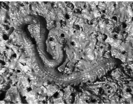
Figure 1.4 – The ragworm

Nereis diversicolor

………..……….…..………... 21

Chapter 2

Figure 2.1 - Comparison between velocities measured (ADV) and predicted (CFX) for the 10

cm width flume, at 5 and 10 cm s

. Lower graph showing the benthic boundary layer in detail

……….……….….. 46

Figure 2.2 - Hydrodynamic conditions in the flumes a) measurements in the NIOO flume with

ADV; b) CFX simulations for the IMAR flume ...……….………….…… 47

Figure 2.3 - Relationship between shear velocity u

estimations (using LW method) and

current velocity (U), in the IMAR and NIOO flumes corresponding to the following linear

regressions (u

= 0.2462U+0.0141, R

=1.0) and (u

= 0.0267U+0.1008, R

=0.96) ….…….… 48

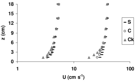
Figure 2.4 - Velocity profiles at 5 and 40 cm s

measured over a smooth surface (S), the

control sediments (C) and cockles bed (Ck) in the NIOO flume ………..…… 48

Figure 2.5 - Relationship between current velocity (U) and shear velocity (u

) for a smooth

surface (S), control sediments (C) and cockles bed (Ck) in the NIOO flume ………..…….... 49

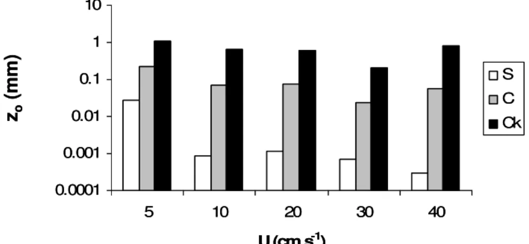
Figure 2.6 - Roughness length (z

) over increasing U in a smooth surface (S), over the control

sediments (C) and cockle bed (Ck) in the NIOO flume. z

axis is in a logarithmic scale for a

Figure 3.1 – Side-view of the artificial cockle beds using the two density of shells M (500 ind

m

) and H (1000 ind m

) and the three roughness levels, T4 being the roughest and T2 the

smoothest. The distance between two crosses of the white board is 5 cm …..……...……….. 67

Figure 3.2 -

Cerastoderma edule

changes in topographical roughness, measured as element

height (k, cm), over increasing free-stream velocities (u

, cm s

) for the natural treatments.

Lines refer to linear regressions for each treatment as: black broken line (C), solid grey line

(M) and solid black line (H). Legends as in Table 3.2 ..………... 69

Figure 3.3 –

Cerastoderma edule

changes in topographical roughness, measured as element

height (k, cm), over increasing free-stream velocities (u

, cm s

) for the natural treatments.

Lines refer to linear regressions for each treatment as: black broken line (C, control), solid grey

line (M, 500 ind m

) and solid black line (H, 1000 in m

)……...………..….. 73

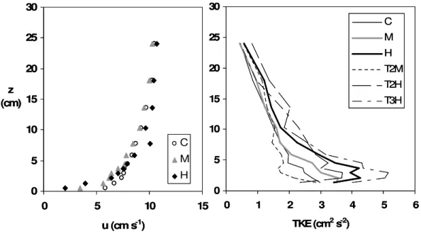
Figure 3.4 –

Cerastoderma edule

effect in the BBL. Average velocity profiles (u, cm s

, U of

~ 10 cm s

) and turbulent kinetic energy profiles (TKE, cm

s

, at U of ~ 25 cm s

). Each

profile is an average of 8 individual sub-profiles. Legends as in Fig. 3.3.………..………….. 75

Figure 3.5 –

Cerastoderma edule

effect in the relationships between shear velocity (u

) and

free-stream velocity (U) for comparable treatments. Individual points represent averages of 8

sub-profiles. Legends and functions of the relationships can be found in Table 3.2……...….. 76

Figure 3.6 –

Cerastoderma edule

effect in the relationships between turbulence kinetic energy

(TKE, cm

s

) and the square of free-stream velocity (U

) for comparable treatments.

Individual points represent averages of 8 sub-profiles. Legends and functions of the

relationships can be found in Table 3.2. ………..……. 78

Figure 3.7 –

Cerastoderma edule

effect in the relationships between normalised turbulence

kinetic energy (TKE

) and shear velocity (u

) for comparable treatments. Individual points

represent averages of 8 sub-profiles. Legends as in Table 3.2………..….... 78

Figure 3.8 –

Cerastoderma edule

effect in the relationships of normalised TKE (TKE

) as a

function of roughness or element height (k). Treatments are gathered in two groups: one with

live

C. edule

(M and H,

♦

) and the second with the treatments without live organisms (C and T

treatments,

฀

)……….……….………...… 79

Figure 3.9 -

Cerastoderma edule

effect on turbulence (TKE averaged in the first 6 cm from the

bed) as a function of individual clearance rate (CR) of a population of 280 ind m

, average

shell length and weight of 26 mm ± 2 and 0.16g ± 0.01. Linear regression presented in the

figure. ……… 80

Figure 3.10 -

Cerastoderma edule

jet length scale (z

, cm) and clearance rates (CR, L h

ind

(TKE

) as a function shear velocity (u

) for the control treatments of Exp. 1 (C,

○

) and of

Exp. 2 (Ct,

฀

) and the lowest density of

C. edule

(280 ind m

, L, *), medium (500 ind m

, M,

▲

) and the highest density (1000 ind m

2, H,

♦

).……… 81

Chapter 4

Figure 4.1 - A: Annular flume used to study the effects of bioturbation by

Nereis diversicolor

on the resuspension of sediment exposed to different current velocities. B: Experimental setup

(view across the flume channel). (adapted from Sobral & Widdows, 2000) ……..………….. 95

Figure 4.2 - a) Aspects of the sediment surface at the beginning of the incubation period (day

0). Note, on the upper microcosms, the trace of a

N. diversicolor

burrowing. b) Sediment

surface at day 20, in the control treatment. It is possible to observe the developed biofilm;

lighter shaded areas on the surface correspond to sediment from lower layers, transported to the

surface by the meiofauna. (photos from experiment MAR) ………. 96

Figure 4.3 - Effect of free stream velocity (cm s

) on eroded matter (E

) (g m

)(± SD)

(symbols) and on the content of OM on E

(lines) for experiments NOV (A) and MAR (B), for

the controls (CNOV and CMAR) and the treatments with

N. diversicolor

(N350, N530 and

N790). Symbols with arrows represent the average U

(cm s

) of each treatment...…...…. 100

Figure 4.4 - Eroded chl

a

(g m

) (symbols) and chl

a

content of eroded matter (mg chl

a

g

dw) (lines), as a function of the free stream velocity, for experiments NOV (A) and MAR (B).

Legends as Fig 6.3 ……….…………..….…. 101

Figure 4.5 - Variation of U

(cm s

) and sediment shear strength before erosion s

(kPa) for

both experiments NOV and MAR. Linear regression is based on all data points (F= 8.16,

p<0.01, n=15). Legends as Fig. 6.3 ……….…..…….…… 103

Figure 4.6 - Variation of E

(g m

) and sediment shear strength after erosion s

(kPa) for both

experiments NOV and MAR. Lines indicate linear regression tendency for each experiment.

Legends as Fig. 6.3 ………..……...… 103

Chapter 5

Figure 5.1 - Comparison between the 570 density of

N. diversicolor

(570) and respective

control (Ct 570) for the luminophores concentration profiles found after 21 incubation days, in

terms of a) luminophores concentration, b) the percentage of standard deviation over the

respective average, and c) 570 concentrations with respective control subtraction ………... 125

Figure 5.2 – Profiles of luminophores concentration in depth estimated over time after

bioturbation of

N. diversicolor

for densities of 320, 450 and 570 ind m

………... 128

Figure 5.3 - Biodiffusion coefficients over the bioturbation period for a population of

N.

diversicolor

of 320, 450 and 570 ind m

(± standard deviation) estimated using M1 and M2

Exp. 3) for the different densities of

N. diversicolor

(320, 450 and 570 ind m

) (± standard

deviation) ………..………….. 130

Figure 5.5 - a) Calculations of Db for the 570 Ct treatment using the same concentrations but

different sampling time. b) Calculations of Db for 570 treatment using the profile

concentrations measured over the sampling period, but assuming these profiles were taken at a

fixed time of 3 days ……….……...…. 131

Figure 5.6 – Comparison between the observed profiles of luminophores (o) and predictions

from method M1 (bold line) and M2 (striped line) for each replicate taken on day 21 for 450

and 570 ind m

and 570Ct and for day 20 to 320 ind m

………..………….... 133

Figure 5.7 - Non-locality index measured after 21 days (20 days for 320 density) in the three

densities tested (and control for 570 density) and 450 and 320 density …………..…….….. 135

Chapter 6

Figure 6.1- Map of Tagus estuary (Portugal). A. Sediment collection; B. organisms

collection………..……….... 146

Figure 6.2 - Shear strength (KPa) profiles for each sediment before erosion runs: control (B),

sediment with

N. diversicolor

(N), copper spiked control (CB) and copper spiked sediment

with

N. diversicolor

(CN). Mean

±

SD. n=3. Significant differences among the four sediments

(two-way ANOVA F

=19.0410, p<0.001) and sediment layers (two-way ANOVA

F

=19.9465, p<0.001) ………..……….151

Figure 6.3 - Eroded matter (E

, g m

) in a log scale as a function of shear velocities (u

, cm s

). Lines represent the exponential relationships (expressed on Table 2) in each sediments:

control (B ), sediment with

N. diversicolor

(N ), copper spiked control (CB ) and

copper spiked sediment with

N. diversicolor

(CN ). n=3 ………..………... 155

Figure 6.4 – Input of chlorophyll

a

(mg m

) to the water column at selected shear velocities

(u* cm s

) for control sediment (B), sediment with

N. diversicolor

(N), copper spiked control

(CB) and copper spiked sediment with

N. diversicolor

(CN). Mean

±

SD. n=3 ...…….…….157

Figure 6.5 - Input of dissolved and particulate copper (dCu and pCu, µmol m

) to the water

column at selected shear velocities (u

, cm s

) for copper spiked control sediment (CB) and

copper spiked sediment with

N. diversicolor

(CN). Mean

±

SD. n=3...………..……… 158

Figure 6.6 - Relation between erosion depth (E

, mm) and sediment shear strength (KPa)

measured after erosion. Circle indicates sediments without

N. diversicolor

. Trend line was built

combining data from each sediment (F

=53.98. p < 0.001), control (B), copper spiked

control (CB), sediment with

N. diversicolor

(N) and copper spiked sediment with

N.

Figure 7.1 – Profiles of luminophores concentration over a period of 21 days for a

N.

diversicolor

density of 570 ind m

. The “N” treatment represents

N. diversicolor

in natural

sediment, while “CN” refers to

N. diversicolor

in Cu contaminated sediment. (Bars denote ±

standard deviation) ………..……… 176

Figure 7.2 – Evolution of the biodiffusion coefficient over a period of 21 days. “N” represents

N. diversicolor

in natural sediment, while “CN” refers to

N. diversicolor

in Cu contaminated

sediment. M1 and M2 refer to the different procedures of Db estimation. (Bars represent ±

standard deviation) ……….………. 178

Figure 7.3 – Non-locality index estimated over time for a population of

N. diversicolor

under

natural (N) and contaminated sediments (CN). (± Standard deviation) ………..………….. 178

Figure 7.4 – Depth profiles of luminophore concentration after 21 days for a

N. diversicolor

Chapter 2

Table 2.1 – Characteristics for IMAR and NIOO experiments in terms of a) organisms, b)

experimental conditions, c) flume characteristics and d) sampling conditions... 43

Chapter 3

Table 3.1 - Flume characteristics ………...………...……. 68

Table 3.2 – Topography characterised by the elements height (k, cm, ± standard deviation, n

~10) and by roughness length (z

, cm) in all treatments (C for control (n=10), treatments with

live

C. edule

(n=10): M for 500 ind m

density and H 1000 ind m

and for the artificial

treatments (n=5), the highest roughness level T4 until the lower roughness level T2 for

densities M and H). Relationships between hydrodynamic parameters: shear velocity (u

, cm s

), free-stream velocity (U, cm s

) and turbulence kinetic energy (TKE, cm

s

) (n=10 in C, M

and H and n=5 in T treatments) and normalised TKE (TKE

) ………….……...………. 74

Chapter 4

Table 4.1 - Changes in the shear strength

s

(

±

SD) of the surface sediment after the 20 day

incubation period (s

), and after erosion of the sediment surface (s

) for the experiments NOV

(CNOV and N350) and MAR (CMAR , N 530 and N 790). Also shown are values of SPM,

Em

, eroded OM, eroded chl

a

and erosion rates at the maximum current velocity tested (~50

cm s

)………...………….. 98

Table 4.2 - Additional cumulative effect of bioturbation (Be, %) on: sediment shear strength

(kPa) before (s

) and after (s

) resuspension; critical erosion velocity (U

,);

Em

; erosion rate;

eroded chl

a

and

μ

g chl

a

g

DW for the highest experimental velocity (~50 cm s

) for the

three

N. diversicolor

average densities (N350, N530 and N790 ind m

) ………..……... 99

Table 4.3 - Exponential regressions of SPM (y) (mg l

) on current velocity (x) (cm s

). Also

shown are critical current velocities (U

) required to increase the SPM above a threshold of

50 mg l

(

±

SD) ………..…….…… 99

Chapter 5

Table 5.1 – Biodiffusion coefficient values (cm

Table 6.1 – Biogeochemical characteristics of the sediment before erosion: Control (B),

sediment with

N. diversicolor

(N), copper spiked control (CB) and copper spiked sediment

with

N. diversicolor

(CN). mean

±

SD, (

n,

number of samples) ..………..……. 150

Table 6.2 –Parameters of the fitted equation E=a.e

* for eroded matter, E

, (g m

) and

erosion rates, E

, (g m

s

) as a function of shear velocity, u

(cm s

), and critical shear

velocities (u

cm s

, mean

±

SD, n=3), in the control sediment (B), sediment with

N.

diversicolor

(N), copper spiked control (CB) and copper spiked sediment with

N. diversicolor

(CN). (R

, n=24) .……….………... 154

Chapter 7

Table 7.1 – Db (cm

PART I

GENERAL INTRODUCTION

Introduction

INTRODUCTION

There is a present international concern about ecosystem water quality as well as sea-level rise and erosion of coastal margins, caused by increase of rainfall and storm episodes due to global climatic change. Coastal zone management has gained more attention and has been included in several international commitments (UN Framework Convention on Climate Change, UN Convention on Biological Diversity, UN Convention on Combating Desertification, International Strategy for Natural Disaster Reduction), the Kyoto and Montreal protocols, initiatives such as World Summit on Sustainable Development, Global Earth Observation System of Systems initiative (GEOSS), Intergovernmental Panel on Climate Change (IPCC).

One of the main objectives of the FP7- Specific Program for Environment (including Global Changes)1 is to promote sustainable management of the natural and human environment and its resources by advancing our knowledge on the interactions between the biosphere, ecosystems and human activities, and developing new technologies, tools and services for monitoring, prevention and mitigation of environmental pressures and risks including on health and for the sustainability of the natural and man-made environment, in order to address in an integrated way global environmental issues. Douvere and Ehler (2009) focus on the growing awareness of the need to establish marine spatial planning (as in land use management) and reviewed the international and legal framework relevant to the development of an ecosystem-base sea use management.

Estuaries (semi-enclosed coastal bodies of water) are areas of high biological productivity and have been attractive areas for population establishment for centuries. The consequent pressure of unsustainable and uncontrolled industrial and anthropogenic development creates conflicts with natural processes that sustain the health and productivity of coastal areas and results in situations of contamination and eutrophication and situations of loss or accretion of margins due to erosion and sedimentation.

the upper flats according to water inundation during the tidal cycle. The typology of intertidal mudflats can be characterised in terms of tidal range, wave energy, sediment supply, steepness, bed forms, organic content and biology (Dyer, 1998).

Intertidal mudflats are areas of high production of flora and fauna. They support large populations of birds and form nurseries and feeding areas for coastal fisheries. They are also known as places of high organic matter mineralization (Middelburg et al., 1996; Guarini et al., 2000; Heip et al., 2001), and they constitute an important component in global biogeochemical cycles. Additionally, these zones of high sedimentation are a potential trap for solid phase contaminants. The sedimentation of contaminated sediments, chemical reactions and dissolution under anaerobic conditions (observed in few mm depths in some cases) and resuspension events (leading to recontamination events) are processes that need to be clarified.

The increasing anthropogenic pressures on the environmental systems and the need for sustainable management tools, led to an extensive research focusing on contaminated sediments. Toxicity towards the benthos is another important issue considering their importance at the lower levels of the trophic chain, and considering the contamination amplification to higher levels of the food web and ultimately to human consumption.

1.1 Cohesive sediments

Estuarine sediments are composed of sand (non-cohesive sediments) and mud (cohesive sediments). The non-cohesive sediments can be characterised by being inert material whose transport/erosion/deposition behaviour is mainly determined by physical properties such as gain size distribution (Berlamont et al., 1993). In this case, particle adhesion is due to water-film surface tension. The cohesive sediment particles are characterised for being chemically very reactive. Due to its wide variability of origins and composition the prediction of behaviour, transport and fate of cohesive sediments is much more complex than the non-cohesive.

The granular size and composition are of prime importance for the mechanical behaviour of sediments (in transport, flocculation, erosion, deposition and consolidation). The textural classification of gravel-free muddy sediments was revised by Flemming (2000), who proposed the most recent and more precise diagram using the sand/silt/clay ratio. The chemical properties of organic matter (organic polymers, colloids or dissolved organic carbon) in the liquid phase are also very important for the cohesive behaviour of sediments by influencing the formation of aggregates and flocs. In general, the amount of organic matter is well correlated and proportional to the clay content (Winterwerp and van Kestereren, 2004). According to these authors, there is a group of organic substances that can be regarded as flocculants (polysaccharides, proteins composed of peptides and amino acids) a second group that is neutral (lipids, hydrocarbons like cellulose, lignin composed of aliphatic and aromatic hydrocarbons), and a third group that are dispergents or deflocculants (humic acids). These polymers occur as charged, or as neutral particles and can adsorb to clay particles through van der Waals forces, bipolar forces or hydrogen bonding (Winterwerp and van Kestereren, 2004).

1.2 Sediment dynamics

The cycle of sediment dynamics, also known by the ETDC cycle (erosion, transport, deposition and consolidation) is a present concern considering that the pollutant dynamics of an estuary is closely linked to the distribution of particulate mater. Therefore, the knowledge of the processes governing sediment dynamics is essential to a better prediction and management.

The sediment particles along with seston are transported in the flowing water. The trajectory of each particle follows laminar flows and turbulent eddies. In their trajectories particles collide with other particles and form aggregates with subsequent adherence among particles of cohesive sediment. These aggregates, or flocs, can collide with each other causing floc break-up.

The sediments are transported in suspension in the water column as long as current velocities exceed critical values for deposition. The critical velocity for deposition is dependent on the shape and the height of the floc, i.e. the flocs in suspension do not deposit at the same time or with the same settling velocity.

and floc break-up. The lower the current velocities, the higher deposition rates are observed. Once the particles or flocs are deposited on the seabed, they can either be buried by subsequent deposited sediments or they can be resuspended if current velocity increases. Underneath the deposited sediments there is an increasing pressure that pushes the sediment down and promotes the expulsion of interstitial water as the consolidation process take place. When the current velocities increase and exceed the critical erosion velocity, the consolidated sediments are eroded and brought back in to the water column where they become exposed to turbulent eddies, floc break-up and further aggregation.

Because of their reactivity, mobility and nutritional value, suspended particles have an important role in biogeochemical cycles in estuaries as transfer vehicles of chemical constituents between water column, bed sediment and food chain (Fig. 1.1).

Figure 1.1 - Schematic representation of the role of suspended sediments in estuarine biogeochemical processes. Boxes represent compartments hosting materials and chemical constituents, and arrows denote physical and biogeochemical processes responsible for the transfer of such between compartments (Turner and Millwards, 2002).

feeders on sediment and nutrient dynamics have but a description of suspension-feeding activity and other ecophysiological variables (Sohma et al., 2001, 2008; Turner and Millwards, 2002). Due to the multidisciplinary range of processes and their interactions, the clear relevance of each process (within the scale of observation) on sediment dynamics is still not clear.

1.2.1 Transport

The physical processes that dominate sediment transport in aquatic ecosystems are relatively well defined (e.g. Mehta et al., 1989; Houwing, 1999; Gleizon et al., 2003; Dyer et al., 2004). Sediment transport is governed by an advection-dispersion equation for the mass conservation of suspended sediments:

C

K

C

U

t

C

∇

∇

=

∇

+

∂

∂

[1]

where C is the suspended sediment concentration (kg m-3) and t is time (s).

t C

∂

∂ _{expresses the}

accumulation rate in time and space. U is the free stream current velocity (m s-1_{) and K is the}

dispersion coefficient (m2 s-1).

The description of transport is only completed after considering bottom exchanges by erosion and deposition rates. Erosion and deposition are sources and sinks that started to be taken in to account recently (Brenon and Le Hir, 1999; Cancino and Neves, 1999; Cugier and Le Hir, 2000). These two processes will be discussed in detail later.

The structure of the flow is characterised by shear flow near the bed (Fig. 1.2). At the bottom, there is a benthic boundary layer (BBL) characterise by a velocity gradient developed between U in the water column and the boundary, where no slip- condition applies (i.e. at z=0, U=0). Within the part of the turbulent boundary layer, the velocity profile is logarithmic and may be described by the Prandtl von Karman equation or “law of the wall”:

=

0

z z u z U

κ [2]

of the logarithmic velocity profile (u (z) versus ln (z)) and z0 is estimated from the intercept

between the relation (u(z) versus ln (z)) and the Y-axis.

Figure 1.2 – Schematic drawing of a benthic boundary layer (BBL) in parallel flow at zero incidence.

Shearing stresses within the benthic boundary layer of a flow (∂u/∂z) are a

manifestation of the drag force at the bed and the flux of momentum per unit area per unit time is known as the bed shear stress (τ, Pa). The modelling approaches used to estimate erosion and deposition rates are dependent on τ and its critical values at which erosion or deposition start (Houwing, 1999). Therefore, τ is one of the most important parameters used in the modelling of sediment transport in the benthic boundary layer and in evaluation of the benthic flux of material.

Most numerical models using hydrodynamic parameters are based on empirical

formulas assuming τ as a quadratic function of shear velocity (u*, m s-1) τ ∝ u2 (Winterwerp

et al., 2006), or using the Manning roughness coefficient (Dias and Lopes, 2006) or the Nikuradse roughness coefficient to express topographical roughness (Houwing and Van Rijn, 1998; Lumborg, 2005, Zimmermen et al., 2008).

The estimation of τ is normally performed using indirect approaches and the properties of the sea bed are frequently disregarded, which reduces the accuracy of its

velocity (U) height

(z)

BBL

0

velocity (U) height

(z)

BBL

determination and the accuracy of hydrodynamic models. Therefore the knowledge on the parameters of the BBL over natural structures needs to be developed.

Some efforts have been taken by El Ganaoui et al. (2004) to discriminate the erosion and deposition behaviour of the top “fluff layer” and of the deeper sediment. They have showed that multi-class models, using two critical shear stresses for erosion and deposition dependent on sediment characteristics, have a better fit to observed data.

1.2.2 Erosion

Sediment erosion is an important component of sediment dynamics. It produces a source of sediment to the water column, but also nutrients, organic matter and contaminants. From the theoretical point of view, the mechanical processes of sediment erosion are well described. A review of the calculation methods to estimate erosion rates was performed by Mehta et al. (1982). The formulations for erosion rates (ER, kg m-2 s-1) are based on the concept of critical bed shear stress. Erosion happens when τb > τe , which means that erosion

occurs as long as the applied bed shear stress (τb, Pa) is larger than the critical bed shear

stress for erosion (τe, Pa). ER is then described as:

n e

b

z

z

M

ER

=

τ

−

τ

where M(z) is an empirical erosion coefficient with its dimension depending on an exponent

n, τe(z) is the critical bed shear stress for erosion that may vary with z.

Sanford and Maa (2001) revised the mathematical formulation for erosion and proposed a suitable assumption that neglected M and τe while setting n = 1, and derived the

previous formulation [2] to:

0

0

t t e

b

d

z

e

ER

=

ρ

β

τ

−

τ

where ρd(z) is dry bulk density at sediment depth z, β is a local parameter, τe0 is critical bed

shear stress when τb is first applied at t = t0, t is time (h), and γ =dτe dz is the vertical gradient of the critical bed shear stress.

biological factors influencing them, are an unknown function of sediment depth (Aberle et al., 2004).

There are known linear relationships between ER and sediment characteristics such as dry bulk density, water content, mud/sand content, organic content, colloidal carbohydrate (Houwing, 1999, 2000; Friend et al., 2003; Aberle et al., 2004). Friend et al. (2003) verified that the use of Chlorophyll a sediment content as a proxy for τe is related to seasonal

variability for intertidal silty sand sediments of the Ria Formosa. This relationship would only be suitably used for late summer/early autumn.

In 2004 Winterwerp and Van Kesteren proposed a formulation for ER that would incorporate some mechanical sediment characteristics:

d e b E

M

ER

=

τ

−

τ

ρ

and

SS

d

c

M

50 0

10

φ

=

ME (m/Pa-1s) is an erosion parameter, cv (m2 s-1) is the consolidation coefficient in vertical

direction,φs,0 (-) is sediment concentration by volume at onset of swell (i.e. the in-situ volume

concentration), 10d50 (µm) median floc size, SS (Pa) undrained shear strength. cv (m2 s-1) is a

function of permeability and compressibility of the skeleton:

g

m

p

c

w v v

ρ

1

=

where p is permeability (m s-1_{), m}

v (m2 N-1) is the compressibility, ρw (kg m-3) the water

density and g gravitational acceleration (m s-2).

Although some efforts have been taken to include properties of the sediment on the description of erosion mechanisms, the relationships that are likely to influence the quantity of eroded matter, are still poorly described. The proper formulation of ER would imply the numerical descriptions of known physical (shear and critical velocities), chemical and biological functions, involved in sediment biogeochemical properties.

of the knowledge gained from these and other works, approaching both advances and shortcomings related to mud sampling and the use of benthic erosion devices.

1.2.3 Deposition

The deposition component of sediment dynamics has received attention from many science fields: in geology, because of the depositional record; in geochemistry areas focusing chemically less permanent deposits and interactions with previously deposited constituents and in biology areas focusing settlement of larvae and food particles to benthic fauna.

Deposition is the gross flux of cohesive sediment flocs on the seabed and sedimentation is the net increase in bed level (Winterwerp and van Kestereren, 2004). Thus, the sedimentation rate is the deposition rate minus the erosion rate.

By definition, sediment is formed of granular material that can settle in water by gravity. Settling velocity of an individual particle (Wd, m s-1) in still water corresponds to the

constant velocity at which particles settle through a static fluid when the resistance of the fluid exactly equals the downward force of gravity acting on the particle. It is dependent on particle density, shape, size, and surface texture, and on the density and viscosity of the fluid. According to the Stokes Law, Wd can be estimated as

µ

ρ

ρ

18

10 2 50 d g

W s w

d

−

= [8]

where ρs is the density of sediment particles (kg m-3), ρw is the density of water (kg m-3), g is

the gravitational field strength (m s-2), 10d50 is the floc size (m) and µ is the dynamic

molecular viscosity of water (kg m-1 _s-1_{). Observations from previous studies show}

relationships between Wd and salinity (van Leussen, 1999). A comparison between Wd

observed on natural sediments and a model prediction using Stokes law show that natural sediments have Wd two orders of magnitude larger (McCool and Parsons, 2004). Techniques

to measure settling velocities of cohesive sediment aggregates were recently reviewed by Mantovanelli and Ridd (2006). They briefly describe a wide variety of devices emphasizing logistical and scientific implications of its use and measuring purposes.

The first particles to deposit are the largest (e.g. aggregates), most dense or closest to the bottom. During deposition, flocs will have high probability of aggregation and collision with other flocs with different Wd. The processes of flocculation (Winterwerp, 2002;

(Jarvis et al., 2005) are a function of shear stress at steady state. Flocculation plays an important role on the vertical transport of sediments towards the bed (Lick et al., 1992) and is important to understand the partitioning between contaminants and the sediment, organic and water phase (Ongley et al., 1992).

Recent approaches using numerical analysis have indicate correlations between the median floc size and sediment concentration (Xu et al., 2008) and provided a new heuristic formula for turbulence induced flocculation of cohesive sediments (Winterwerp at al., 2006).

The present descriptions of deposition in estuaries are mostly based on the characteristics of the hydrodynamics and suspended matter. Realistic numerical simulations of these phenomena’s are complex due to the variety of particle characteristics in time in the water column and the definition of critical shears for deposition of different sediment classes. In addition, there are biologic activities that may influence sediment deposition. For example, the suspended sediment that is removed from the water column by the benthic organisms is transformed and deposited as faeces, i.e. larger aggregates of suspended material (Turner and Millward, 2002).

1.2.4 Consolidation

As mud flocs accumulate on the bed, the flocs that arrived first are squeezed by the ones on the top and suffer a vertical pressure gradient. Pore water is driven out of the flocs and out of the space between the flocs. This process is known as self-weighting consolidation (Winterwerp and van Kestereren, 2004). In the consolidation phase, flocs are mainly supported by particle interactions and are described by the Gibson equation, which is a simple wave equation in vertical direction z, over time t:

(

)

=

0

∂

∂

+

∂

∂

s s s

z

t

ν

φ

φ

[9]

where φ_sis the volumetric solids concentration (kg m-3_{) and}

s

ν is the settling velocity of the

mud flocs (m s-1) relative to a fixed reference plane. The consolidation of cohesive sediments can be expressed as cv, the consolidation coefficient (see section 1.2.2, Equation [7]),

dependent on sediment permeability and compressibility.

usually assessed through measurement of the critical erosion threshold (Teisson et al, 1993; Houwing, 1999) and shear strength (Watts et al., 2003). The relationships between some of these parameters are not clear. The expected trend of increasing shear strength and decreasing porosity with depth was only observed in 31% of drill sites from the entire suite of expeditions from the OceanDrilling Program (Bartetzko and Kopf, 2007).

Although the activity of burrowed organisms is not usually taken into account in the processes of consolidation, there are evidences of the effects of the crab Mictyris longicarpus

(Webb and Eyre, 2004) and the bivalve Yoldia limatula (Ingalls et al., 2000) on sediment

porosity and irrigation.

1.2.5 Sediment stability

Sediment stability is not by itself a component of what is understood to be the dynamic cycle of estuarine sediments. The concept of sediment stability refers roughly to the resistance of cohesive sediments to erosion. It should be understood as a general term, which can be characterised in terms of the properties of the sediment: sediment shear strength, critical erosion shear stress, porosity, grain size, and in terms of the response to shear velocities: erosion rates, critical shear stress.

The effect of biological processes on sediment stability is important in the transport of microbenthos, nutrients, organic matter and contaminants to the water column (Rasmussen et al., 1998; Mazik and Elliot, 2000). In addition, benthic organisms are known to affect sediment stability and other properties such as their effect on sediment strength and erodability (Baillie and Welsh, 1980; Kornman and de Deckere, 1998; Widdows et al., 2000; Blanchard et al., 2001).

1.2.6 Contaminated sediments

Heavy metals bind to clay mineral particles follow the same transport and deposition pattern than other particles, having a negligible transport towards the open sea (Sondi et al., 2008). A recent study focusing on the distribution of contaminants in three shelf areas from the Portuguese coast was published by Mil Homens et al. (2006). They observed that the character of the contaminated sediments transported to these shelf areas is further influenced by grain-size sorting as well as by dilution with other marine sediments.

The effect of floods is an important issue because it is a source of material derived from the runoff of the basin soils, increasing suspended sediments, nutrients and pollutants. Zonta et al. (2005) highlighted the effect of floods on the transport of suspended sediments and contaminants in the estuary of the Dese River (Venice Lagoon). They concluded that the transport of most of the analysed heavy metals was driven by the suspended particulate matter concentration.

There are some studies focusing the effect that macrofauna have on contaminant distribution in the sediments and their input to the water column (Rasmussen et al., 1998; Ciarelli et al., 2000; Delmotte et al., 2007; French and Turner, 2008), but the effect of contaminated sediments on the bioturbation activity of macrofauna was never investigated.

In terms of sediment dynamics, contaminated sediments are normally approached as an object (to be transported, deposited or resuspended), and not as an influencing factor on sediments dynamics. In order to predict the response of mudflats to environmental and anthropogenic pressures, a greater understanding on the multidisciplinary processes that affects sediment dynamics with associated contaminants is needed. So far, the effect of contaminate sediments on sediment stability has not been investigate.

1.3 Biologic interactions with sediment dynamics

A wide diversity of organisms, from bacteria to benthic invertebrates and marsh plants that inhabit the sediment bottom performs a variety of activities that influence sediment physical structure, biogeochemical properties, and species distribution (Hewitt et al., 2006; Rabaut et al., 2007).

maintain and/or create habitats. The distinction between “ecosystem engineers” and “key-stone species”, one whose effect is large and disproportionately large relative to its biomass and abundance (Power et al., 1996) has been widely discussed (Jones et al., 1997; Crain and Bertness, 2006; Wright & Jones 2006 and references within).

The concept of estuarine ecosystem engineers is more applied to plants due to their importance on the processes of fine particles retention and in the promotion of refuge for other macrofauna species influencing the habitat and the distribution of the surrounding community (Brusati and Grosholz, 2006; Hewitt et al., 2006; Neira et al., 2007; Rabaut et al., 2007).

The benthic communities influence sediment dynamics by affecting some components of the ETDC cycle and sediment stability. They are characterized according to size; micro (< 32 µm), meso (>32 µm and < 1 mm) and macrobenthos (> 1 mm) and according to location; hyperbenthos (organisms living above the sediments), epibenthos (living on top of the sediment) and endobenthos (living inside the sediment). They change sediment characteristics and stability, influencing biogeochemistry, bottom topography and velocities near the bed, sediment deposition and in the case of suspension feeders, constitute an additional removal of suspended particles. Although this is a known fact, the quantification of these influences is not properly addressed.

1.3.1 Sediment stabilisers and destabilisers