Todos os direitos reservados.
É proibida a reprodução parcial ou integral do conteúdo
deste documento por qualquer meio de distribuição, digital ou
impresso, sem a expressa autorização do
Less Inequality, More Welfare? A Structural
Quantitative Analysis for Brazil
António Antunes
Tiago Cavalcanti
Juliana Guimarães
Less Inequality, More Welfare? A Structural Quantitative Analysis
for Brazil
António Antunes
Tiago Cavalcanti
Juliana Guimarães
António Antunes Banco de Portugal [email protected]
Tiago Cavalcanti
University of Cambridge and
Sao Paulo School of Economics - FGV [email protected]
Juliana Guimarães
Less Inequality, More Welfare?
A Structural Quantitative Analysis for Brazil
∗
António Antunes
Banco de Portugal ❛♥t✉♥❡s❛❛❅❣♠❛✐❧✳❝♦♠
Tiago Cavalcanti
University of Cambridge and Sao Paulo School of Economics - FGV
t✈❞✈❝✷❅❝❛♠✳❛❝✳✉❦
Juliana Guimarães
Homerton College, University of Cambridge ❥❣❝✷✾❅❝❛♠✳❛❝✳✉❦
Abstract
This article studies how the recent fall in wage inequality in Brazil affected individual allocations and welfare. It first documents the evolution of wage inequality in the coun-try between 1996 and 2009. Then, it constructs a parsimonious structural model of the Brazilian economy, which is based on a standard Yaari perpetual youth model in which agents are heterogenous in their skills and on their idiosyncratic labor productivity. The model is calibrated to match, besides other statistics, the skill wage premium, the share of skilled workers in the labor force and the cross sectional variance on unobservable wage inequality in Brazil in 1996 and 2009. Our simulations show that the fall in wage inequality in Brazil from 1996 to 2009 generated an average welfare gain equivalent to a 2.24 percent permanent increase in annual consumption. The gains were distributed unevenly: While welfare gains were large for poor individuals (e.g., about 16 percent in permanent consumption for the first income decile), workers in the top of the income distribution experienced, in general, welfare losses (e.g, a loss of 6 percent in permanent consumption for the last income decile). Using counterfactual exercises we also study the importance of different structural factors which shaped inequality on individual welfare.
JEL Classification:E21; D91; D63; D31
Keywords: Inequality; Welfare; Brazil
∗ We have benefited from discussions and conversations with Jonathan Heathcote and Gustavo
“While headline economic growth has not been as spectacular in Brazil as in China and India... the balance of income distribution has improved more rapidly in Latin America’s largest economy than in the other large emerging markets.
On the winning side have been an estimated 33m people who since 2003 have risen to the ranks of the so-called “new middle classes” or above...
On the losing side, say sociologists, are the 20m or so people of the “traditional” middle classes...
The process has been driven partly by increasing access to education. The new middle class has flocked to private universities and technical colleges and begun competing for jobs with the traditional middle class.” Financial Times, July 20th, 2011. Brazil’s tale of two middle classes.
1
Introduction
Brazil is one of the most unequal countries in the world. According to the World De-velopment Indicators (WDI) Brazil is actually at the 7th position in the world league of income inequality. The Gini index of income in Brazil (the average value between 2007 and 2009) is 0.5521 and it is on the right tail of the cross-country distribution of the Gini coefficient in the world. In addition, not only the level of inequality is high in the country, but at the same time there is low social intergenerational mobility by international standards (e.g.,Ferreira and Veloso,2006;Dunn,2007).
Brazil, however, was even more unequal in 1996. According to the World Devel-opment Indicators, the average value of the Gini coefficient in Brazil between 1994 and 1996 was equal to 0.604 and Brazil was the third most unequal country in the world. Therefore, contrary to what is observed in most OECD countries, in which the gap between rich and poor individuals has reached its highest level for over 30 years,1
inequality of wages in Brazil has been decreasing sharply in the last 15 years2
(Sec-tion2provides a detailed description of wage inequality in Brazil). See, for instance, Figure1. The conditional skill premium, measured by the returns on education when wages are controlled for other individual characteristics such as age, gender and race, for example, decreased from 140 percent in 1996 to 100 percent in 2009. Not only ob-servable inequality (e.g., individual characteristics such as human capital) has been decreasing over time but also residual inequality (e.g., individual risks), measured by the cross-sectional variance of the residual in a Mincerian regression of wages on individual characteristics, has declined. See the bottom left graph of Figure2. This is in contrast with most evidence on developed countries such as in the United States and in the United Kingdom, where the skill premium has been increasing, despite the
1SeeOECD(2011). Inequality has risen even in traditionally egalitarian countries, such as Germany, Denmark and Sweden.
higher relative supply of skilled workers, as well as idiosyncratic wage volatility.3 In
developed countries inequality has been in the forefront of discussions recently (see
Piketty,2014;Atkinson,2015).
Therefore, Brazil is a very interesting laboratory, since the movements in inequal-ity have been quite different from those observed in developed countries.4 More importantly, due to the fast pace inequality is declining in the country, Brazil has be-come a reference for other developing countries in adopting policies to reduce inbe-come inequality. In addition, in contrast to the literature for the United States, which has a large and growing number of articles on the welfare implications of rising wage inequality,5 there is no study which investigates how changes in the factors which
shaped the Brazilian wage distribution affected individual allocations and welfare.6 This article fills this gap.
Related to our paper is Jones and Klenow (2011), who provide welfare analysis for a cross-section of countries. They do not consider households’ decisions, but they instead use a direct approach by considering measures on consumption, leisure, in-equality, and mortality directly into a utility function. They show that relatively to other countries, welfare in Brazil is reduced by its high level of consumption inequal-ity. However, welfare in the country has increased at a higher rate than income per capita from 1980 to 2000. Heathcote, Storesletten, and Violante(2013), however, ex-plain clearly the importance to use a structural approach rather than a direct approach using observations on the cross-sectional distribution of consumption to evaluate the welfare implications of changes in the wage distribution. The structural approach takes into account the decisions of agents, the costs associated with each decision and therefore the trade-offs individuals face to achieve some outcomes, while the indirect approach does not. This justifies our structural approach to address the question of how changes in wage inequality affected welfare in the country.
We quantify the welfare effects of changes in factors which shaped inequality in Brazil by using a parsimonious structural model of the Brazilian economy. We build a standard Yaari perpetual youth model in which agents face uninsurable risks on labor productivity and credit constraints in the same spirit ofHuggett(1993) andAiyagari
3For the United States, see for instance Heathcote, Storesletten, and Violante(2010), and for the United Kingdom seeBlundell and Etheridge(2010). The changes in inequality in Brazil are not neces-sarily observed in other emerging market countries, such as Russia and Mexico. In Russia residual in-equality has been decreasing but skill premium has been roughly constant (seeGorodnichenko, Peter, and Stolyarov,2010). In Mexico in the 1990s inequality increased over the years (Binelli and Attanasio (2010)).
4Spain had a similar path of inequality (seePijoan-Mas and Sanchez-Marcos,2010).
5See, for instance, Attanasio and Davis(1996),Krueger and Perri(2004),Heathcote, Storesletten, and Violante(2010) andHeathcote, Storesletten, and Violante(2013).
(1994) and in which there are two levels of skills.7 In each period of time there is
a constant mass of agents dying, which is replaced by new agents with equal mass so that population is constant. Agents enter the economy as unskilled workers and can invest in education to acquire skills and therefore become skilled workers. In the main calibration we use data on college education to define a skilled worker. In Ap-pendixAwe base the definition of skilled workers using data on high school degree. We calibrate the model to the Brazilian economy so that we match key moments of the data in 1996 and then perform several counterfactual exercises by changing three structural parameters of the model: (i) The implicit cost of acquiring skills; (ii) the importance of skilled workers in production (skill biased technical change); and (iii) the residual variance of individual wage inequality. We change these structural pa-rameters of the model, such that we match the following statistics of the Brazilian economy in 2009: the skill wage premium, the share of skilled workers in the labor force and the cross sectional variance of unobservable wage inequality. We then cal-culate the percentage in permanent consumption needed to compensate households for being in an economy with the parameters observed in 1996 instead of those ob-served in 2009. The welfare analysis focuses not only on stationary equilibria but also on transitional dynamics.
The main findings were the following: The recent fall in wage inequality in Brazil is equivalent to an increase of 2.24 percent in annual consumption when only station-ary equilibria are analyzed. Calculating transitional dynamics leads to larger welfare gains.8 The gains were distributed unevenly: While welfare gains were large for poor
individuals (e.g., about 16 percent increase in annual consumption equivalent to the baseline for the first income decile), workers in the top of the income distribution ex-perienced, in general, welfare losses (e.g., a loss of 6 percent of consumption equiva-lent to the baseline for the last income decile). Then, in order to calculate the impact of each factor in shaping inequality and welfare, we modified each parameter separately per simulation and compared welfare of each counterfactual economy with respect to the baseline calibration. We found that the large welfare gains were due mainly from the reduction in the barriers to acquire skills and from the reduction in the variance of the residual inequality (or individual wage volatility). The skill-biased technical change, on the other hand, decreased average welfare but its effects were not strong enough to compensate the positive effects of the other two factors. Therefore, overall the recent movement on the factors which shaped inequality in Brazil has benefited mostly poorer individuals, while workers in the top of the income distribution are, in general, worse off.
It is important to emphasize that we abstract from important dimensions of real
7Our model is a simplified version of the model presented byHeathcote, Storesletten, and Violante (2013). We simplified it due to some data restrictions on Brazil, so that we could easily identify the parameters of the model from the data and how they changed over the years using the Brazilian households survey. See alsoHeathcote, Storesletten, and Violante(2014).
life, such as fertility choices, and some policies which might have affected the shape of the wage inequality in Brazil and could have implications to our welfare analysis. We are aware that our approach is not free from model misspecification and thus should be viewed as only an illustration of the potential magnitude of the welfare impacts of the recent changes in wage inequality in Brazil.
Interestingly, American workers have faced opposite movements in wage inequal-ity which are translated into a rising skill wage premium (despite the strong rise in the supply of skilled workers) and an increasing wage volatility. Nevertheless, in model-based calculationsHeathcote, Storesletten, and Violante(2013) surprisingly find that such movements in wage inequality in the United States have generated welfare gains exceeding one percent of lifetime consumption (see alsoHeathcote, Storesletten, and
Violante,2010). Under the new wage structure, however, there are welfare losses on
the lower tail of the wage distribution. Therefore, while the changes in the factors that shaped inequality in the United States have not been pro-poor welfare enhancing, in Brazil that is the case. Our results are robust to different calibrations of the model as shown in AppendixB.
This paper has four more sections. The next section analyzes the movement on wage inequality over 15 years in Brazil using the Brazilian household sample survey. Section 3describes the model economy and defines the equilibrium. Section 4 cali-brates the parameters of the model and provide the counterfactual exercises. The last section contains concluding remarks.
2
Empirical motivation
We start by studying the movements on wage inequality over the past 15 years in Brazil.9 We begin by investigating the variance of individual log wages for our
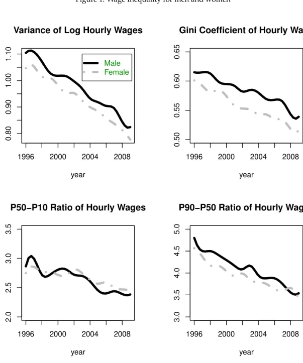
sam-ple of the Brazilian household samsam-ple survey, PNAD (Pesquisa Nacional por Amostra de Domicílios), comprising the period from 1996 to 2009. All estimations were performed for a sample of males and females, separately, aged from 16 to 65 years. As we may notice in the left-upper graph of Figure1, the variance of male and female log wages decreased steadily over the period by around 28 log points. The wage Gini coefficient decreased 12 percent for males (see the right-upper graph of Figure1) and 14 percent for females.
In order to understand this pattern across the distribution, we estimated the ra-tios for the 50th and 10th (P50-P10) percentiles and the 90th and 50th (P90-P10) per-centiles. The patterns are similar for both men and women. The P50-P10ratio (left lower graph in Figure1) had a small decrease over the period, changing roughly by 0.31 points for females and 0.48 for males. The decrease in inequality on the top of the
wage distribution was more accentuated as shown by theP90-P50ratio plots (right lower graph in Figure1). Both for males and females, inequality at the upper part of the wage distribution decreased steadily from 1996 onwards.10 This wage ratio
decreased by approximately 30 percent for both males and females workers.
We now investigate the sources of the fall of wage inequality in Brazil. We estimate the role of some important individual characteristics such as education and age on reducing inequality in the country. The education wage premium was defined as the ratio between the average hourly wage of workers with college degree with respect to those without a college degree. We also estimated the conditional college degree premium as the coefficient for the indicator variable for college degree in a Mincerian wage equation that controls for other observable characteristics.11 Figure2reports the unconditional and conditional skill wage premium. Both measures show a decline in the college wage premium that starts on 1998 for males and a bit later for females. In AppendixAwe also show a similar decline for the unconditional and conditional high school wage premium (See Figure6). The conditional college wage premium for males decreased by roughly 40 percentage points from 1996 to 2009, from 140 percent to 100 percent. With a close look at the data, we notice that in the same period there was an increase in the average level of education in Brazil of almost two years on average. Historically, this increase had been, on average, one year per decade. This is also shown on our plot of the ratio of number of workers with a college degree and number of workers without a college degree for the period, which increased from 3.5 percent in 1996 to about 6.5 percent in 2009 for male workers (see Figure3). This ratio increased even more rapidly for female workers. Using some decomposition techniques,Barros, Carvalho, Franco, and Mendonça(2010b) found that together, the decline in the level of inequality in schooling and also on the premium for schooling over the decade, are responsible for 50 percent of the decline on wage inequality and 30 percent of the decrease in income inequality in Brazil.
We also report the experience wage premium (see the right-upper graph of Figure
2). It was estimated as the ratio between the average hourly wage of 45–55-year-old workers and the hourly wage of 25–35-year-45–55-year-old workers. The male experience premium remained roughly constant over the entire period. However, the experience premium for female workers decreased by more than 20 percent during the period.12
10The decline in inequality in Brazil has received great attention. Barros, Carvalho, Franco, and Mendonça(2010b) analyzed the movements on income inequality and measures of poverty for the pe-riod of 2001-2007. They show that in 2001 the degree of inequality, measured by the Gini coefficient of family income in Brazil was close to the average for the previous 30 years, whereas by 2007 inequality had decreased by 7%. As we show here, it kept declining for the rest of the decade. See alsoBarros, Carvalho, Franco, and Mendonça(2010a).
11The Mincerian wage equation controlled also for experience, gender, race, region of residence within the country and wether or not the worker was a civil servant. We also add an indicator vari-able of whether or not the worker has a formal job and the college wage premium was robust to this variable. See alsoCavalcanti and Santos(2015).
Figure 1: Wage Inequality for men and women
1996 2000 2004 2008
0.80
0.90
1.00
1.10
year
Male Female Variance of Log Hourly Wages
1996 2000 2004 2008
0.50
0.55
0.60
0.65
year
Gini Coefficient of Hourly Wage
1996 2000 2004 2008
2.0
2.5
3.0
3.5
year
P50−P10 Ratio of Hourly Wages
1996 2000 2004 2008
3.0
3.5
4.0
4.5
5.0
year
P90−P50 Ratio of Hourly Wages
Figure 2: College, experience wage premia and residual inequality
1996 2000 2004 2008
3.5
4.5
5.5
year
Male Female College Wage Premium
1996 2000 2004 2008
0.8
1.0
1.2
1.4
1.6
year
Experience Wage Premium
1996 2000 2004 2008
0.9
1.1
1.3
year
Conditional College Wage Premium
1996 2000 2004 2008
0.0
0.4
0.8
1.2
year
raw residual Variance of Residuals
Figure 3: Supply of skilled workers
1996 1998 2000 2002 2004 2006 2008
0.04
0.05
0.06
0.07
0.08
year Male
Female
College to Non−College Ratio
Source: Brazilian household survey (PNAD) and authors’ calculations. Black solid line: Males. Gray dot-dash line: Females.
Finally, the plot for variance of residual inequality, measured as the variance of the residual from a regression of male log wages on workers’ characteristics, shows that the inequality not explained by observable characteristics has also been declining over the sample period (see the right-lower graph of Figure2). In addition, compared to the variance of hourly wages in Brazil, the residual inequality accounts for 60% of the whole male wage dispersion.13
3
The model
3.1
Environment
Time is discrete and index byt =0, 1, 2..., and the economy lives forever.
Demographics: We follow the Yaari perpetual youth model in which agents survive
from age jto j+1 with constant probability δ. In each period, 1−δ agents die, and
constant for males.
an equal mass of agents are born, so that the population remains constant. The mass of population is equal to one and the mass of agents with ageJis equal to(1−δ)δJ.
Preferences and productivity shocks:Let β∈ (0, 1)be the subjective discount factor andct be consumption at period t. Lifetime utility for an agent born in timet = kis
given by:14
U =Ek " ∞
∑
t=k
(βδ)t−ku(ct)
#
. (1)
Expectations are taken over an idiosyncratic shock, zt ∈ Z, on labor productivity,
where
ln(zt+1) =ρln(zt) +ǫt+1, ρ∈ [0, 1]. (2)
Variableǫt+1is an iid shock with zero mean and varianceσǫ2. The one-period utility
function has a constant elasticity of intertemporal substitution, 1σ:
u(c) = c1 −σ
1−σ, σ >0 .
Education: There are two education levels: skilled and unskilled, such that g ∈ S = {s,u}. Unskilled agents have one unit of unskilled labor and can become skilled with
probability pe ∈ [0, 1] if they invest φ in terms of the consumption good in
educa-tion. Therefore, φ corresponds to the cost of acquiring skills. These cost represent
not only monetary costs but also pecuniary costs to acquire skills, which might reflect the education system in the country (e.g., barriers to entry in the education system, regulation). Once skilled, agents can work as skilled or unskilled workers.
Production technology: The consumption good is produced with a CES technology
that uses skilled, S, and unskilled labor, U, as inputs. The technology exhibits con-stant returns to scale and is given by:
Y =AγSθ−θ1 + (1−γ)Uθ−θ1
θ−θ1
, A>0, γ∈ (0, 1), andθ >0 . (3)
The elasticity of substitution between skilled and unskilled labor is equal to θ.
Pa-rameter γ corresponds to the importance of skilled labor in production relative to
unskilled labor.
Asset market: Markets are incomplete as in Huggett (1993) and Aiyagari (1994).
There are no state contingent assets and agents trade a risk-free bond,a∈ A = [a,∞).
Agents have also access to annuities to insure against the risk of survival. At birth agents are unskilled and are endowed with zero financial wealth.
In order to avoid a Ponzi game, we followAiyagari(1994) and use a natural bor-rowing limit.Aiyagari(1994) defines a “natural” borrowing limit as a situation where in an agent’s worst possible state, z, interest payments do not exceed labor income (i.e., current debt can at least be rolled over after a long spell of low productivity shocks). The steady-state natural borrowing limit is given by:15
a′ ≥a =−wuz
r .
3.2
Optimal behavior and equilibrium
Firms: Factor markets are competitive. Profit maximization implies that input prices
are equal to the marginal product of each factor, such that
ws = Aγ
γSθ−θ1 + (1−γ)U θ−1
θ
θ−11
S−θ1, (4)
wu = A(1−γ)
γSθ−θ1 + (1−γ)Uθ−θ1
θ−11
U−θ1. (5)
Therefore, the skill premium is given by:
ws
wu =
γ
1−γ
U
S 1θ
, (6)
which is decreasing in the skilled to unskilled labor ratio, S
U. It also depends on the
importance of skilled workers in production,γ.
Households: The problem of an unskilled agent with financial wealth a and labor productivity shockzis to choose consumption,c, next period level of financial wealth, a′, and whether or not to invest in education,e, to maximize:
vu(a,z,λ) = max
c,a′,e{u(c) +βδE[epevs(a
′,z′,
λ′) + (1−epe)vu(a′,z′,λ′)]}, (7)
subject to
c+δa′+φe = wu(λ)z+ (1+r(λ))a, (8)
lnz′ = ρlnz+ǫ′, ǫ′ ∼iidN(0,σǫ2), (9)
λ′ = H(λ) (10)
c≥0, a′ ≥ a(λ), ande∈ {0, 1}. (11)
15See, for instance,Antunes and Cavalcanti(2013) for a formulation of this restriction during a tran-sition. They also show that the shape of the borrowing limit (e.g., natural,ad-hocor endogenous) does
Equation (8) is the one-period budget constraint, equation (9) defines how the id-iosyncratic shock evolves over time, and equation (11) describes the restriction on the choice variables. Observe that the household’s value function depends not only on the current idiosyncratic state and asset holding, but also on aggregate variables such as the wage of skilled and unskilled labors, which are affected by the aggregate mea-sureλ. To compute such measure in the next period, the households need to know
the current period’s entire measureλ, and an aggregate law of motion, which we will
callH, such thatλ′ = H(λ). We will define H(·)shortly.
Analogously, the problem of a skilled agent can be summarized by the following equations:
vs(a,z,λ) = max
c,a′ {u(c) +βδE[vs(a
′,z′,λ′)]}, (12)
subject to
c+δa′ = ws(λ)z+ (1+r(λ))a, (13)
lnz′ = ρlnz+ǫ′, ǫ′ ∼iidN(0,σǫ2), (14)
λ′ = H(λ) (15)
c ≥0, and a′ ≥ a(λ). (16)
Equilibrium:The state space is defined byM =A×Z×S. The typical element ofM
ism ∈ M. LetχA andχZbe the associated Borelσ-algebra ofA andZ, respectively.
LetP(S)be the power set forS. DefineΩM =χA⊗χZ⊗P(S)as theσ-algebra onM;
therefore,(M,ΩM) is the corresponding measurable space. For each B ∈ ΩM, λ(B)
corresponds to the mass of households whose individual state vectors lie inB.
The policy functions associated with problem (7) area′u =hau(a,z,λ),cu =hcu(a,z,λ)
and e = he(a,z,λ). The policy functions associated with problem (12) are a′s =
has(a,z,λ) and cs = hcs(a,z,λ). Define Q(m,λ,B;h) as the endogenous transition
probability of the households’ state vector. It describes the probability that a house-hold with statem = (a,z,g ∈ {s,u})will have a state vector lying in Bnext period, given the current asset distributionλand a vector of decision rulesh. Therefore,
Q(m,λ,B;h) =
∑
(h(m,λ),z′)∈B
Prob(z′ ∈ Z|z)δ+
∑
(h(m=(0,z,u),λ),z′)∈B
Prob(z′ ∈ Z|z)(1−δ).
The aggregate law of motion implied by transition function Q is an object T(λ,Q) that assigns a measure to each Borel setB. It can be computed as
T(λ,Q)(B) =
ˆ
M
Q(m,λ,B;h)dλ. (17)
Note thatλ′(·) = T(λ,Q)(·). We now define a stationary recursive competitive equi-librium.
and vs(a,z,λ); set of price functions {r(λ),wu(λ),ws(λ)}; firm decision rules U(λ) and
S(λ); and aggregate function H(λ), such that:
(i) Given price functions r(λ), wu(λ) and ws(λ) and aggregate function H(λ),
opti-mal decision rules hau(a,z,λ), hcu(a,z,λ), he(a,z,λ) are associated to value function
vu(a,z,λ).
(ii) Given price functions r(λ), wu(λ) and ws(λ) and aggregate function H(λ), optimal
decision rules has(a,z,λ)and hcs(a,z,λ)are associated to value function vs(a,z,λ).
(iii) Given price functions wu(λ)and ws(λ), firm decision rules U(λ)and S(λ)maximize
profits.
(iv) Markets clear:
U =
ˆ
M,g=u
zdλ (18)
S =
ˆ
M,g=s
zdλ (19)
0 =
ˆ
M,g=u
hau(a,z,λ)dλ+ ˆ
M,g=s
has(a,z,λ)dλ, (20)
Y =
ˆ
M,g=u
(hcu(a,z,λ) +φhe(a,z,λ))dλ+ ˆ
M,g=s
hcs(a,z,λ)dλ. (21)
(v) Distributions are consistent with individual behavior: H(λ)coincides with T(λ,Q).
4
Quantitative experiments
The purpose of the quantitative analysis is to assess numerically the impact of the changes in inequality on welfare in Brazil. The exercises require us to firstly calibrate the theoretical model (i.e., determine values for a set of parameters for preferences, technology, the stochastic process on labor productivity, and education costs). We choose parameter values consistent with empirical observations for male workers in Brazil in 1996. We consider male workers only for the following reason: the male labor force participation and the average number of hours worked by male workers remained roughly the same over the period of analysis,16 while female labor force
participation increased continuously in the same period. Therefore, the inclusion of female workers would require us to build a different framework to account for the increase in female labor participation and the fertility transition.
Once parameters are calibrated, we change three structural parameters (c.f., cross-sectional variance on residual inequality, importance of skilled workers in produc-tion, and costs to acquire skills) so that the model economy is consistent with three statistics related to inequality (c.f., skilled to unskilled workers ratio, skill wage pre-mium and individual wage volatility) for the 2009 data. We then compare welfare of the 1996 baseline economy with the economy that matches 2009 statistics. We also perform counterfactual analysis to understand the role of each factor in welfare.
This approach has at least three caveats. The first is that when we match the statistics in 2009, we are implicitly assuming that in that year the economy is in the stationary equilibrium. This is of course not necessarily the case, but the exercise of subsection4.2.2shows that the transition is relatively fast, with the three prices (r,wu
andws) within 5% of their long run values after 13 years. This assumption simplifies
the analysis and it might underestimate welfare (losses) gains, since wage inequality is still falling. Although in recent years inequality has reduced at a lower speed.
The second shortcoming is that we are assuming that all three parameters change instantaneously in the first year, and then the economy will adjust to the new station-ary equilibrium. While we have experimented with more gradual transitions in the parameters, with results that are not far from those reported here, this would imply that we could not calibrate the model for the 2009 data for the reason explained in the first caveat.
Finally, changing three particular parameters to attain three different data targets implies that we are selecting the type of structural changes that led to the observed changes in those targets. However, this is a parsimonious model, and the unchanged parameters control for other aspects of the model economy, which are not directly related to changes in the labor market and in access to education.17
4.1
Calibration
We now describe how the value of each parameter was set. The time period of the model is set to be 1 year. We choose the surviving probabilityδsuch that the expected
life time during adulthood is equal to 50 years. This implies thatδ =0.98.
Utility: Risk aversion coefficient σ is set at 2.0,18 which is consistent with micro
ev-idence in Mehra and Prescott (1985). The subjective discount factor β was chosen
such that the real risk free interest rate is about 4.0 percent. The calibrated value was
β = 0.9054. This is lower than the real interest rate on Brazilian Treasury bonds, which has been around 6 to 7 percent according to the Brazilian Central Bank. But it
17For instance, parameterσdetermines the elasticity of intertemporal substitution in consumption; and parameterθdetermines the elasticity of substitution between skilled and unskilled labor.
is important to emphasize that this is the interest rate on risk free bonds, while the Brazilian Treasury rate reflects also Brazil’s unstable macroeconomic past and any country specific risk, which was not negligible in the 1990s and up to the first half of the last decade.
Stochastic process on labor productivity:For the idiosyncratic process, we followed
Krueger and Perri(2005). We use a finite approximation of the following
autoregres-sive process
ln(z′) = ρln(z) +ǫ′, (22)
whereǫ′is normal iid with zero mean and variance σǫ2. We approximate it using a 9
state Markov process spanning 3 standard deviations of the log wage (seeTauchen,
1986). Since there is no household panel for Brazil comparable with the Panel Study of Income Dynamics (PSID) in the United States, we do not have estimates for the persistence parameterρ.19 As a result, we setρ equal to 0.98, which is a value
con-sistent to what is observed in the United State. See, for instance,Krueger and Perri
(2005).20 Table6in AppendixBcontains sensitivity analysis to all parameters
deter-mined outside the model (σ, θ, ρ, pe and δ), including the persistence parameter ρ.
We show that welfare results are in general robust to local variations in all exogenous parameters. For the cross-section variance of idiosyncratic income we use the PNAD data and estimate it by removing the effects of observable variables in a Mincerian equation, as explained in section2. The value for 1996 for this cross-section variance in the male regression isσz2 = σǫ2
1−ρ2 =0.621 (see the lower-right graph of Figure2).
Production and education variables: We set the elasticity of substitution between
skilled and unskilled labor to be equal toθ = 1.5, which is a number reported in the literature.21 SeeKrusell, Ohanian, Ríos-Rull, and Violante(2000). Then we chose pa-rameterγand education costφjointly such that we match the following two statistics: 19There is thePesquisa Mensal de Emprego(PME) in Brazil which is a longitudinal wage data in Brazil. However, individuals in this survey stay in the sample for a maximum of 16 months and since our model period is one year, we cannot estimate with precision the persistence of yearly idiosyncratic shocks in Brazil.
20In a recent paper,Kaplan and Violante(2010) show that Bewley models with a highly persistent parameter (above 0.97) display an average level of consumption smoothing that is consistent to what is observed in the data. Since wage mobility in Brazil is low by international standards (e.g.,Ferreira and Veloso,2006; Dunn, 2007), we should expect a higher value for ρ. Higher values for ρ lead to larger welfare gains of reducing wage inequality and therefore our simulations produce conservative welfare numbers. See part I of Table6in AppendixB.
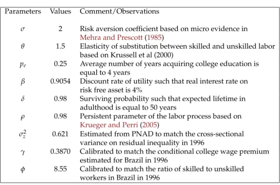
Table 1: Parameter values, baseline economy
Parameters Values Comment/Observations
σ 2 Risk aversion coefficient based on micro evidence in Mehra and Prescott(1985)
θ 1.5 Elasticity of substitution between skilled and unskilled labor based on Krussell et al (2000)
pe 0.25 Average number of years acquiring college education is
equal to 4 years
β 0.9054 Discount rate of utility such that real interest rate on risk free asset is 4%
δ 0.98 Surviving probability such that expected lifetime in adulthood is equal to 50 years
ρ 0.98 Persistent parameter of the labor process based on Krueger and Perri(2005)
σz2 0.621 Estimated from PNAD to match the cross-sectional
variance on residual inequality in 1996
γ 0.3870 Calibrated to match the conditional college wage premium estimated for Brazil in 1996
φ 8.55 Calibrated to match the ratio of skilled to unskilled workers in Brazil in 1996
the conditional college wage premium, which is equal to 140 percent (see the lower-left graph of Figure 2); and the ratio of college workers and non-college workers, which is equal to 3.5 percent (see the left graph of Figure3). The calibrated values are: γ =0.3870 andφ =8.55.22 The probability to become skilled, pe, is chosen such
that the average number of years in acquiring college education is 4 years, which implies that pe = 0.25. Table 1 reports the values of all parameters and contains a
comment on how they were selected.
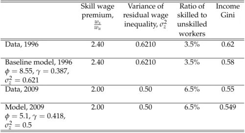
Table2shows that all calibrated statistics were matched including the skilled wage premium and the skilled to the unskilled workers ratio. The 1996 Gini index of in-come in the model is equal to 0.58, while in the data it is equal to about 0.62. However, notice that in the model the sources of inequality are the idiosyncratic risks on labor productivity and the skill premium, while in the data there are other factors in shap-ing inequality, such as race and age, among others.
The last row of Table2shows the statistics of the model economy when we match the 2009 moment for the skill wage premium, the variance of the residual wage in-equality and the skilled to unskilled workers ratio. The model matches well all statis-tics for the 2009 data. Notice that to match these statisstatis-tics observed in 2009, the vari-ance of the idiosyncratic shocks decreased from 0.6210 to 0.50 (a reduction of 20%);
Table 2: Selected statistics data and model
Skill wage Variance of Ratio of Income premium, residual wage skilled to Gini
ws
wu inequality,σ 2
z unskilled
workers
Data, 1996 2.40 0.6210 3.5% 0.62
Baseline model, 1996 2.40 0.6210 3.5% 0.58 φ=8.55,γ=0.387,
σz2=0.621
Data, 2009 2.00 0.50 6.5% 0.55
Model, 2009 2.00 0.50 6.5% 0.549
φ=5.1,γ=0.418, σz2=0.5
Sources: statistics constructed using the 1996 and 2009 PNAD microdata.
the relative importance of skilled workers in production increased from 0.387 to 0.418 (an increase in 8%); and the implicit cost to acquire skills reduced from 8.55 to 5.1 (a reduction in 40%). Although there was an important decrease in the relative wage of skilled workers it was mainly caused by the sharp increase in supply of skilled work-ers in the labor force, and not because recent technological change has not been skill-biased.23 Quite the opposite, since γ has increased in the period and technological
change has also been skill-biased in Brazil. Interestingly the Gini index in the model decreased from 0.58 in the baseline to 0.549 with the parameters of 2009. This implies a 5.61 percent decrease in the Gini coefficient. In the data in the same period the Gini Index decreased from 0.62 to 0.55, which corresponds to a 11.29 percent decrease in this index. Therefore, the model accounts for roughly 50 percent of the decrease in the Gini coefficient in this period. This is consistent with the findings ofBarros, Carvalho,
Franco, and Mendonça(2010b) who using decomposition techniques show that the
decline in level of inequality in schooling and its premium explain about 50 percent of the decline in wage inequality in Brazil.
4.2
Welfare
4.2.1 Stationary equilibria
Now we perform counterfactual exercises using the calibrated model to investigate how welfare changed in Brazil due to the changes in different factors which shaped the recent movements in inequality in the country.24 Results are reported on Table3. Firstly, we jointly changed the following three parameters: (i) the cost to acquire skills,
φ; (ii) the importance of skilled workers in production,γ; and (ii) the variance of the
idiosyncratic shock,σz2 = σǫ2
1−ρ2 - we keep ρconstant and changeσ
2
ǫ. We change them,
such that we matched the following statistics of the Brazilian economy in 2009: the skill wage premium, the ratio of skilled to unskilled workers and the cross sectional variance on unobservable wage inequality. The second row in Table3 contains the results of this experiment. Observe that the income Gini index decreases by more than 5 percent. It falls from 0.58 to 0.55. The interest rate increases since there is less precautionary savings with the reduction in idiosyncratic risks. A higher interest rate increases welfare in the top of the wealth distribution but reduces it in the bottom of this distribution, since asset rich agents have a large fraction of their earnings coming from interest income.
Quantitatively, the welfare implications are large and the effects are asymmetric across the income distribution.25 We report an average welfare measure, which is
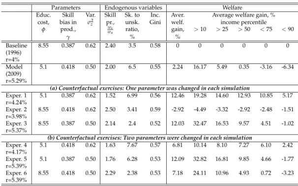
a weighted average of the welfare gains (losses) of all agents in the economy. This aggregate welfare gain is about 2.24 percent of permanent consumption equivalent of the baseline economy when these three parameters are changed so that we match key statistics of the Brazilian economy in 2009. This implies that on average workers in Brazil would need to be compensated by an increase in 2.24 percent of permanent consumption to be in an economy with a level of inequality similar to that observed in 1996, instead of the one observed in 2009.26 This is a substantial measure when compared to important supply-side reforms.27 Table3also reports the welfare
impli-24We calculate the consumption equivalent, µ, for the benchmark economy and for the economy after the change in some parameters relative to the baseline, such that(1+µ)1−σv1996
g −v2009g = 0,
g=s,u. We compare welfare by income deciles.
25We measure the welfare by the average permanent consumption supplement (e.g., Lucas,1987) that makes households in an economy with benchmark parameters value as well off as in an economy with some specific parameter change.
26Table5in AppendixAprovides the welfare implications of the changes in the wage distribution in Brazil when we define skilled workers by those with a high school degree. Welfare gains are much larger than those presented here. So we could see this number as a conservative measure of the impact of changes in the wage distribution on welfare in Brazil.
Table 3: Welfare analysis and counterfactual exercises
Parameters Endogenous variables Welfare
Educ. Skill Var. Skill Sk. to Inc. Aver. Average welfare gain, % cost, bias in σz2 pr., unsk. Gini welf. income percentile
φ prod., ws
wu ratio, gain, >10 >25 >50 <75 <90
γ % %
Baseline 8.55 0.387 0.62 2.40 3.5 0.58 0 0 0 0 0 0 (1996)
r=4%
Model 5.1 0.418 0.50 2.00 6.5 0.55 2.24 16.17 5.49 0.35 -3.16 -6.34 (2009)
r=5.29%
(a) Counterfactual exercises: One parameter was changed in each simulation
Exper. 1 5.1 0.387 0.62 1.52 6.99 0.56 12.46 19.28 14.60 12.93 10.85 5.17 r=4.24%
Exper. 2 8.55 0.418 0.62 2.50 3.41 0.59 -2.92 -4.49 -3.32 -2.92 -2.48 -1.51 r=3.98%
Exper. 3 8.55 0.387 0.50 2.14 2.4 0.52 12.03 32.47 16.53 9.57 4.51 -1.02 r=5.37%
(b) Counterfactual exercises: Two parameters were changed in each simulation
Exper. 4 5.1 0.418 0.62 1.63 7.67 0.57 6.81 10.14 8.10 7.27 6.10 2.42 r=4.17%
Exper. 5 5.1 0.387 0.50 1.76 6.28 0.53 12.09 32.82 16.81 9.85 4.66 -1.77 r=5.39%
Exper. 6 8.55 0.418 0.50 2.29 2.38 0.53 7.18 24.11 10.96 4.93 0.72 -3.23 r=5.39%
cations per income decile. For agents in the bottom of the income distribution there are large welfare gains coming mainly (as we will see next in the counterfactual ex-ercises) from the reduction in the barriers to acquire skills and from the reduction in the variance of idiosyncratic shocks. Agents are worse off in the top of the income distribution. For those workers welfare decreased substantially. Although the cost to acquire skills decreased, skill premium also decreased, which reduced welfare of agents in the top of the income distribution.
Figure 4 displays a three dimensional graph of the welfare gains. The welfare gains are on thez-axis, while thex-axis andy-axis contain labor earnings (in logs), and worker asset holdings, a, respectively. Quantitatively, households with a low labor income and low net wealth position benefit considerably from the changes in the factors that shaped the recent fall in inequality in Brazil. For other households with a high level of labor earnings and positive asset position, the changes in inequality have been welfare reducing. Therefore, overall the recent movement on inequality in Brazil has benefited mostly relatively poorer workers, while workers in the top of the income distribution are, in general, worse off. The movements in inequality in Brazil increased slightly the unskilled wage and reduced the skilled wage. In addition, the distribution of the idiosyncratic shocks became less disperse. Such changes tend to keep average consumption constant and reduce consumption inequality. Under an utilitarian welfare measure, this increases average welfare since marginal utility is
Figure 4: Welfare gains per asset holdings and idiosyncratic shock
−2
−1 0 1
0
1
2
3
4
−10 0 10 20 30 40
assets average welfare gains (in percentage)
labor earnings (in logs)
higher for workers in the bottom of the earnings distribution.
Next, we perform counterfactual exercises in order to investigate the role of each factor in shaping the overall welfare gains. We divide these counterfactual exercises into two sets: (a) we change only one parameter in each experiment; and (b) we change two parameter in each experiment. Those are pure counterfactual exercises and would try to capture the dynamics of the economy if for instance only the cost of acquiring skills had changed while the other parameters, such as labor income risks and the production function, would have remained at their initial value. In the first counterfactual exercise we decreased only the value of the cost to acquire skills, such that the value is similar to the implicit value calculated for 2009. Notice that as a consequence of lower costs to acquire skill, the fraction of skilled to unskilled workers in the labor force increases, which in turn decreases the skill wage premium. Inequality in income decreases. There is an average welfare gain of 12.46 percent of consumption equivalent to the baseline. Welfare increases across all income deciles but the gains are mainly concentrated at the lower tail of the income distribution. The concentration of welfare on the lower tail of the income distribution is explained by two facts: (i) some agents who were unskilled with a lower cost to acquire skill could now invest in education and therefore can enjoy a higher permanent income and consumption level; and (ii) in equilibrium the unskilled wage increases with a lower barrier to acquire skills and consequently higher supply of skilled workers.
0.387 to 0.418, which as discussed previously indicates a skill-biased technical change in Brazil in this period. Average welfare reduces by 2.92 percent of consumption equivalent to the baseline and there are welfare losses across all percentiles of income. In equilibrium, the unskilled wage decreases, reducing welfare. The losses are mainly concentrated in the lower tail of the income distribution.28 This experiment suggests that the skill-biased technical change has benefited only a small fraction of agents in the economy, but overall it has had a negative effect on welfare.
Experiment 3 reports the exercise in which we only change the cross-sectional variance on residual inequality, such that instead of matching the value observed in 1996 (σz2 = 0.62), we match the value observed in 2009 (σz2 = 0.5). We kept the value of the other parameters at those observed in 1996. Notice that income inequality de-creases substantially by more than 10 percent, since the Gini index decreased from 0.58 to 0.52. The interest rate rises substantially since there is less precautionary sav-ings. Average welfare increases by 12.03 percent of consumption equivalent to the baseline and the welfare gains are mainly concentrated at the bottom of the income distribution. For agents in the bottom decile of income, for instance, average welfare gains from reducing idiosyncratic variance from 0.62 to 0.5 are large, corresponding to an increase in permanent consumption of 32 percent of the baseline value. On the other hand, for agents in the top decile of the income distribution the average welfare loss is about 1 percent of consumption equivalent to the baseline level.
We then perform counterfactual exercises in which we changed two parameters per simulation instead of only one. In experiment 4, we change both the cost to ac-quire skills and the relative importance of skilled workers in production. In experi-ment 5 the parameters changed were the cost to acquire skills and the variance of the idiosyncratic shocks. Finally, experiment 6 reports the case in which we changed the importance of skilled workers in production and the variance of residual inequality. All parameters are changed from their baseline value to the value observed in the 2009 model economy. These exercises confirm previous findings that the reduction in the barriers to acquire skills and on the variance of the residual inequality were important factors in shaping the recent movement in inequality in Brazil. Moreover, they have contributed substantially to improvements in welfare in the country and in particular the welfare of those workers who are in the bottom of the income distribu-tion.
4.2.2 Transitional dynamics
Comparing welfare of two stationary equilibria is a valid exercise. It is as if we were evaluating the welfare of two economies with different characteristics and therefore we can analyze who is better off or worse off by income brackets. In evaluating the welfare effects of the changes in the factors which shaped the recent movements in
Figure 5: Transitional dynamics: Prices and welfare
−2
−1 0
1 0
2 4 0
20 40 60
assets average welfare gains (in percentage)
labor earnings (in logs) 0 10 20 30
1 1.02 1.04 1.06 1.08 1.1 1.12 1.14
t
w u
unskilled wage
0 10 20 30
2 2.1 2.2 2.3 2.4
t
w s
skilled wage
0 10 20 30
0.04 0.045 0.05 0.055 0.06 0.065
t
r
interest rate
equality in Brazil it is also important to investigate the transitional dynamics. Firstly, the median agent, for instance, in the initial stationary distribution is not necessar-ily the same median agent in the final stationary distribution, and this is true for all agents ranked according to the wealth or income distribution. There is social mobility in the economy and comparing value functions of two different stationary equilibria for agents at the same point of the wealth or income distribution might be mislead-ing. We therefore calculate each agent’s value function considering the transition from one stationary equilibrium to another. Also, the adjustment on prices might be slow and therefore abstracting from such adjustments might lead to different values of welfare.29 Are our results robust when we consider transitional dynamics?
Figure5plots the adjustments of prices (unskilled and skilled wages and interest
rate) from the baseline economy to an economy with the all the three parameters (c.f. cost to acquire skills, importance of skilled workers in production, and variance of the idiosyncratic shocks) with values observed in 2009. Figure5 shows that it takes about 10 years for prices to be close to their long-run level.30 The transition of the
unskilled wage and of the interest rate are not monotonic. The unskilled wage firstly increases because there is a jump in the number of workers deciding to acquire skills. Then, the unskilled wage decreases to a value that is about 0.10 percent larger than the baseline value. The skilled wage decreases monotonically from its initial value of 2.4 to its final stationary level of 1.99. The interest rate rises in the transition and stays above the initial stationary level since there is less precautionary savings due to a decrease in idiosyncratic wage volatility.
The first graph of Figure5displays a three dimensional plot of the welfare gains. Observe that the shape of the welfare gains (losses) is similar to the one in which we consider only stationary equilibria (see Figure4). Welfare gains are concentrated on the lower tail of the net wealth and income distributions and welfare losses are ob-served in relative rich (in asset and income) workers. However, gains are larger and losses are smaller when we consider transitional dynamics than when we do the anal-ysis using only stationary equilibria.31 The average welfare gain when we consider
transitional dynamics is about 6.34 percent of consumption equivalent of the baseline economy when the three parameters are changed so that key statistics of the Brazilian economy in 2009 are matched. This is about 2.8 times the average welfare measure when we consider only stationary values. For agents in the bottom decile of income, the average welfare gains from changing the factors that shaped the recent move-ments in inequality in Brazil corresponds to an increase in permanent consumption of about 24 percent of the baseline value (instead of 16 percent when we abstract from transitional dynamics). For agents in the top decile of the income distribution the av-erage welfare losses is about 4.31 percent of consumption equivalent to the baseline level (instead of an average welfare loss of 6.34 percent).
Finally, notice that we are comparing the value of each parameter in two different points in time. However, the changes that we observed in the cost to acquire skills, on the importance of skilled workers in production, and on the idiosyncratic wage volatility did not necessarily happen in such a discrete and profound way. Important reforms and policies were implemented in Brazil during the period of analysis, but the changes in the parameters of the model might have happened with a smoother adjustment. We have experimented with more gradual transitions in the parameters, with an average welfare gain larger than those reported here when we consider tran-sitional dynamics.32 One important issue is that for each point in time the vector
30We assume a rapid change in the parameters, which implies that the economy is very close to the stationary equilibrium in 2009.
31This is explained by the movement in prices during the transitional dynamics. Both the unskilled wage and the skilled wage are higher in the transition than at their final long-run level.
of the labor productivity shocks changes. In addition, the model does not necessar-ily match the observed endogenous statistics (e.g., skill wage premium and share of skilled workers in the labor force) in 2009. An alternative is to change parameters such that they match the endogenous related variables, but this would require us to basically calibrate the model in each point in transition, which is extremely demand-ing for this class of models.
5
Concluding remarks
This paper firstly documents how wage inequality evolved in Brazil in the last 15 years. In particular, it shows the evolution of the skill wage premium, cross-sectional variance on observed and unobserved wage inequality and the change in the stock of skilled workers in the labor force. Then, it develops a structural model of the Brazil-ian economy in which agents are heterogenous in their skills and face uninsurable idiosyncratic shocks to labor productivity. The simulations show that the fall in wage inequality in Brazil from 1996 to 2009 generated an average welfare gain equivalent to a 2.24 percent permanent increase in annual consumption.33 The gains were
dis-tributed unevenly: While welfare gains were large for poor individuals (e.g., about 16 percent in permanent consumption for the first income decile), workers in the top of the income distribution experienced, in general, welfare losses (e.g, a loss of 6 percent in permanent consumption for the last income decile). Overall the recent movement on the factors which shaped inequality in Brazil has benefited mostly rel-atively poorer workers, while individuals in the top of the income distribution are, in general, worse off.
Using counterfactual exercises we also study the importance on welfare of differ-ent structural factors which shaped inequality in the country. Our exercises show that the large welfare gains we found were due mainly to the reduction in the bar-riers to acquire skills, and to the reduction in the variance of the residual inequality (or individual wage volatility). The skill-biased technical change, on the other hand, decreased average welfare but its effects on welfare were not strong enough to com-pensate the positive effects of the other two factors.
Our analysis abstracts from government transfers to the poor, such as the Bolsa
Famíliaprogram. We consider only wage income, and how the factors that shaped
the movement on wage inequality in Brazil affected individual welfare. Given the importance of cash transfers for poor households, we might expect even larger
wel-1996 to the value in 2009. In this experiment it takes 6 periods for the value ofφ,γandσǫ2to converge to the 2009 value. In each period the change in the parameter is the same. For instance,φdecreased by 0.575 in 6 periods. The average welfare gain of this experiment is about 12 percent of a permanent increase in annual consumption.
fare gains if we had considered the changes in income inequality rather than wage inequality. In a recent article, Berriel and Zilberman (2011), focusing on the Bolsa Famíliaprogram, provide a welfare analysis of conditional cash transfers in Brazil in a model with idiosyncratic shocks and incomplete markets. They find that the condi-tional cash transfers program in Brazil increased average welfare by about 3.2 percent of consumption equivalent to an economy without cash transfers when transitional dynamics are considered, but about 0.3 when only stationary equilibria are evalu-ated. Therefore, not only the changes in wage inequality in Brazil were pro-poor welfare-enhancing, but also some adopted government social policies. While the
Oc-cupy movementagainst social and economic inequality in rich countries, such as the
United States and the United Kingdom, might be justified due to raising inequality and individual wage volatility, in Brazil workers can still complain about the level of inequality, which is still one of the highest in the World, but not about its trend.
References
AIYAGARI, S. R. (1994): “Uninsured Idiosyncratic Risk and Aggregate Saving,” Quar-terly Journal of Economics, 109(3), 659–684. 3,10,11
(1995): “Optimal Capital Income Taxation with Incomplete Markets, Borrow-ing Constraints, and Constant Discount Factor,”Journal of Political Economy, 103(6), 1158–1175. 18
ANTUNES, A., AND T. CAVALCANTI(2013): “The Welfare Gains of Financial
Liberal-ization: Capital Accumulation and Heterogeneity,”Journal of the European Economic Association, 11(6), 1348–1381. 11,18
ANTUNES, A., T. CAVALCANTI, AND A. VILLAMIL(2013): “Costly Intermediation &
Consumption Smoothing,”Economic Inquiry, 51(1), 459–472. 18
ATKINSON, A. B. (2015):Inequality: What Can Be Done? Harvard University Press. 3
ATTANASIO, O., ANDS. J. DAVIS(1996): “Relative Wage Movements and the
Distri-bution of Consumption,”Journal of Political Economy, 104(6), 1227–1262. 3
BARROS, R. P., M. CARVALHO, S. FRANCO, ANDR. MENDONÇA(2010a): “Declining
Inequality in Latin America: a Decade of Progress?,” in Markets, the State, and the Dynamics of Inequality in Brazil, ed. by L. F. Lopez-Calva,andN. Lustig. Brookings Institution Press and UNDP. 6
(2010b): “Determinantes da queda da desigualdade de renda no Brasil,” Working Paper 1460, IPEA. 6,17
BEHAR, A. (2010): “The Elasticity of Substitution between Skilled and Unskilled
BERRIEL, T. C., AND E. ZILBERMAN(2011): “Targeting the Poor: A Macroeconomic
Analysis of Cash Transfer Programs,” Mimeo, Pontifícia Universidade Católica do Rio de Janeiro. 25
BEZERRA, J., AND T. CAVALCANTI (2009): “Brazil’s Lack of Growth,” inBrazil under Lula, ed. by W. Baer,andJ. Love. Palgrave. 5
BINELLI, C. (2015): “How the Wage-Education Profile Got More Convex: Evidence
from Mexico,”B.E. Journal of Macroeconomics, 15(2), 509–560. 15
BINELLI, C., AND O. ATTANASIO (2010): “Mexico in the 1990s: The Main
Cross-Sectional Facts,”Review of Economic Dynamics, 13(1), 238–264. 3
BLUNDELL, R., AND B. ETHERIDGE (2010): “Consumption, Income and Earnings
In-equality in Britain,”Review of Economic Dynamics, 13(1), 76–102. 3
CASELLI, F.,ANDW. J. COLEMAN, II (2006): “The World Technology Frontier,” Amer-ican Economic Review, 96(3), 499–522. 15,32
CAVALCANTI, T., ANDA. P. VILLAMIL(2003): “The Optimal Inflation Tax and
Struc-tural Reform,”Macroeconomic Dynamics, 7(3), 333–362. 19
CAVALCANTI, T. V., AND M. R. D. SANTOS (2015): “(Mis)Allocation Effects of an
Overpaid Public Sector,”Mimeo, University of Cambridge. 6
DUNN, C. E. (2007): “The Intergenerational Transmission of Lifetime Earnings:
Ev-idence from Brazil,” The B.E. Journal of Economic Analysis & Policy, 7(2), Contribu-tions, article 2. 2,15
ENGERMAN, S. L.,ANDK. L. SOKOLOFF(2012):Economic Development in the Americas since 1500: Endowments and Institutions. Cambridge University Press. 2
FERREIRA, F. H. G., P. G. LEITE, ANDJ. A. LITCHFIELD(2008): “The Rise and Fall of
Brazilian Inequality, 1981-2004,”Macroeconomic Dynamics, 12(S2), 199–230. 3
FERREIRA, F. H. G., P. G. LEITE, AND M. RAVALLION (2010): “Poverty Reduction
without Economic Growth? Explaining Brazil’s Poverty Dynamics, 1985-2004,” Journal of Development Economics, 93(1), 20–36. 5
FERREIRA, S.,ANDF. VELOSO(2006): “Intergenerational Mobility of Wages in Brazil,”
Brazilian Review of Econometrics, 26(2), 181–211. 2,15
FIRPO, S. P., G. GONZAGA, AND R. NARITA(2003): “Decomposição da Evolução da
GONZAGA, G., N. MENEZES-FILHO, AND C. TERRA (2006): “Trade Liberalization
and the Evolution of Skill Earnings Differentials in Brazil,” Journal of Development Economics, 68(2), 345 ˝U367. 3,9
GORODNICHENKO, Y., K. S. PETER, AND D. STOLYAROV (2010): “Inequality and
Volatility Moderation in Russia: Evidence from Micro-Level Panel Data on Con-sumption and Income,”Review of Economic Dynamics, 13(1), 209–237. 3
HEATHCOTE, J., K. STORESLETTEN, ANDG. VIOLANTE(2010): “The Macroeconomic
Implications of Rising Wage Inequality in the United States,” Journal of Political Economy, 118(4), 681–722. 3,5
(2013): “From Wages to Welfare: Decomposing Gains and Losses from Rising Inequality,” inAdvances in Economics and Econometrics: Theory and Applications, ed. by D. A. M. Arellano,andE. Dekel, vol. 2, pp. 235–282. Cambridge University Press.
3,4,5,17
(2014): “Consumption and Labor Supply with Partial Insurance: An Analyti-cal Framework,”American Economic Review, 104(7), 2075–2126. 4
HELPMAN, E., O. ITSKHOKI, M.-A. MUENDLER, AND S. J. REDDING (2012): “Trade
and Inequality: From Theory to Estimation,”NBER Working Paper No. 17991. 9
HUGGETT, M. (1993): “The risk-free rate in heterogeneous-agent
incomplete-insurance economies,” Journal of economic Dynamics and Control, 17(5-6), 953–969.
3,10
ISSLER, J. V., AND N. S. PIQUEIRA (2000): “Estimating Relative Risk Aversion, the
Discount Rate, and the Intertemporal Elasticity of Substitution in Consumption for Brazil Using Three Types of Utility Function,”Brazilian Review of Econometrics, 20(2), 201–239. 14
JONES, C. I., AND P. KLENOW (2011): “Beyond GDP? Welfare across Countries and
Time,”Mimeo, Stanford University. 3
KAPLAN, G.,AND G. L. VIOLANTE(2010): “How Much Consumption Insurance
Be-yond Self-Insurance?,”American Economic Journal: Macroeconomics, 2(4), 53–87. 15
KRUEGER, D., ANDF. PERRI(2004): “On the Welfare Consequences of the Increase in
Inequality in the United States,”NBER Macroeconomics Annual 2003, p. 83. 3
KRUEGER, D., ANDF. PERRI (2005): “Understanding Consumption Smoothing:
KRUSELL, P., L. OHANIAN, J.-V. RÍOS-RULL, AND G. L. VIOLANTE(2000):
“Capital-Skill Complementarity and Inequality: A Macroeconomic Analysis,”Econometrica, 68(5), 1029–1053. 15,32
LUCAS, JR, R. E. (1987):Models of Business Cycles. Basil Blackwell, Oxford. 18
(1990): “Supply-side economics: an analytical review,” Oxford Economic Pa-pers, 42(2), 293–316. 18
(2000): “Inflation and Welfare,”Econometrica, 68(2), 247–274. 18
MEHRA, R., AND E. C. PRESCOTT (1985): “The Equity Premium: A puzzle,”Journal of Monetary Economics, 15, 145–162. 14,16
OECD (2011):Divided We Stand: Why Inequality Keeps Rising. OECD: Paris. 2
PIJOAN-MAS, J., AND V. SANCHEZ-MARCOS (2010): “Spain is Different: Falling
Trends of Inequality,”Review of Economic Dynamics, 13(1), 154–178. 3
PIKETTY, T. (2014): Capital in the Twenty-First Century. Harvard University Press. 3
TAUCHEN, G. (1986): “Finite-State Markov Chain Approximations to Univariate and
Vector Autoregressions,”Economics Letters, 20, 177–181. 15
A
High school premium
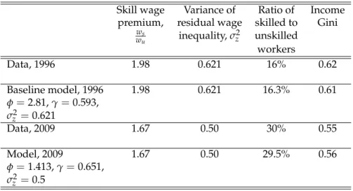
In Section2we investigate the education wage premium by comparing workers with and without a college degree. In this appendix, we compare workers with and with-out a high school degree. This is important in the mapping of some key statistics of the data to the model in order to consider the robustness of our results to another definition of skilled workers. Here we defined skilled workers as those with a high school degree.
Figure 6: High school wage premium
1996 1998 2000 2002 2004 2006 2008
3.0
3.5
4.0
year
Male Female
High School Wage Premium
1996 1998 2000 2002 2004 2006 2008
0.65
0.70
0.75
0.80
0.85
0.90
0.95
year
Conditional High School Wage Premium
Source: Brazilian household survey (PNAD) and authors’ calculation. Black solid line: Males. Grey dot-dash line: Females.
Figure 7: Supply of skilled workers
1996 1998 2000 2002 2004 2006 2008
0.20
0.25
0.30
0.35
year
Male Female HS to Non−HS Ratio
Table 4: Selected statistics data and model
Skill wage Variance of Ratio of Income premium, residual wage skilled to Gini
ws
wu inequality,σ 2
z unskilled
workers
Data, 1996 1.98 0.621 16% 0.62
Baseline model, 1996 1.98 0.621 16.3% 0.61 φ=2.81,γ=0.593,
σz2=0.621
Data, 2009 1.67 0.50 30% 0.55
Model, 2009 1.67 0.50 29.5% 0.56
φ=1.413,γ=0.651, σz2=0.5
Sources: statistics constructed using the 1996 and 2009 PNAD microdata.
supply of the two type of skills were similar from 1996 to 2009, however, the initial levels were substantially different.
We now study the implications for the welfare changes when we define skilled workers as those with a high school degree instead of limiting the skilled worker definition to those with a college degree. The model we consider here is similar to the one presented in Section 3. Ideally we would endogenously introduce the two decision of skills (high school degree and college degree) within the model. We do not follow this approach for two reasons. First, the model would become much harder to solve since it would increase the state space and its dimension. In addition, we believe that the model presented in Section3describes well the trade-off of acquiring or not a college degree (should or not individuals give up some income today for future increases in their wage?) while a high school degree depends also on the choice of parents, which are not explicitly modelled in our framework. Therefore, we see this more as a robustness exercise to our previous findings when we broaden our definition of skilled workers. We choose parameters value such that we match the unobservable inequality, the (high school) skill wage premium, the fraction of (high school) skilled workers in the labor force and the real interest rate for the Brazilian economy. The parameters we changed relative to those presented in Table1were: β, γ, andφ. For instance, the cost of acquiring skills in 1996 is nowφ = 2.81 instead of