Simulation and Calibration Between Parameters of Continuous
Time Random Walks and Subdifusive Model
†A.P.P. PEREIRA1*, J.P. FERNANDES2, A.P.F. ATMAN3 and J.L. ACEBAL4
Received on November 23, 2016 / Accepted on April 17, 2017
ABSTRACT.We address the problem of subdiffusion or normal diffusion to perform a calibration between simulations parameters and those from a subdiffusive model. The theoretical model consists to a general-ized diffusion equation with fractional derivatives in time. The data generated by simulations represents continuous-time random walks with controlled mean waiting time and jump length variance to provide a full range of cases between subdiffusion and normal diffusion. From simulations, we compare the accuracy of two methods to obtain the diffusion constant and the order of fractional derivatives: the analysis of the dispersion of the variance in time and an optimized fitting of the histograms of positions with theoretical model solutions. We highlight the connection between the parameters of the simulations those of theoretical models.
Keywords:anomalous diffusion, fractional diffusion equation, calibration.
1 INTRODUCTION
Anomalous diffusion has been attracting the attention of the scientific community due the large plethora of natural systems which display large deviations from normal diffusion, as plasma diffusion [3], fluid flow in porous media [7, 22], diffusion in fractal structures [23], turbulence [8] etc. Differently to the normal diffusion, associated to local, short range correlations, the presence of long range correlations lead to non-Gaussian probability density functions (PDF).
†Trabalho financiado pelo Cefet-MG e apresentado no CNMAC 2016.
*Corresponding author: Ana Paula de Paiva Pereira – E-mail: [email protected]
1Departamento de Matem´atica, UNIFEI (Campus Itabira), R. Irm˜a Ivone Drumond, 200, 35903-087 Itabira, MG, Brasil. Modelagem Matem´atica e Computacional, PPGMMC-CEFET-MG, Av. Amazonas, 7675, 30510-000 Belo Horizonte, MG, Brasil. E-mail: [email protected]
2Departamento de Engenharia El´etrica, CEFET-MG, Av. Amazonas, 7675, 30510-000 Belo Horizonte, MG, Brasil. E-mail: [email protected]
3Departamento de F´ısica e Matem´atica, CEFET-MG, Av. Amazonas, 7675, 30510-000 Belo Horizonte, MG, Brasil. Instituto Nacional de Ciˆencia e Tecnologia de Sistemas Complexos, INCT-SC, Rua Dr. Xavier Sigaud, 150, 22290-180 Rio de Janeiro, RJ, Brasil. E-mail: [email protected]
In the class of problems generically called anomalous diffusionsome or anomalous Brownian motions, the microscopic kinetics is characterized by increasing probabilities to observe large steps, causing non-Gaussian PDF with heavy tales, or conversely, to observe large waiting times elapsed between steps causing non-Gaussian PDF, causing non-Gaussian PDF with light tales. From a macroscopic point-of-view, those anomalous diffusion processes do not fit in the classical diffusion description by a Fokker-Planck equation for the evolution of the PDFu(x,t)in space and time [11, 24].
As a direct consequence of the central limit theorem, Markov processes displays a linear evolu-tion of the mean square displacement with time,x2(t) ∝ Dt, featuring the normal, or Brow-nian, diffusion [25]. According to that theorem, if the single variable PDF has finite second moment, the cumulative density functions (CDF) is also gaussian.
On the other hand, if the PDF has long-range tails, determining the divergence of the second moment, the L´evy-Gnedenko limit theorem states that the CDF is L´evy distributed, meaning that it has long-range tails too [9]. Alternatively, the q-central limit theorem states that, in the same conditions for the PDF, aq-Gaussian CDF with 1<q <3 is obtained [27]. Those process are generally characterized by a non-linear dependence of the mean square displacement in time, withx2(t) ∝ Dtα [17]. According to the value of the exponentα, the anomalous processes can be classified as sub-diffusive(0 < α <1)or super-diffusive(1 < α < 2)[17]. A relation between the diffusion exponentαand theqparameter was proposed by Bukman and Tsallis [26], and recently verified experimentally [6].
Random walks flight simulations can be generalized as continuous time random walk (CTRW) which are able to simulate processes displaying anomalous diffusion. In particular, considering a random distribution of step lengths as well a random distribution on waiting times, it is possible to control the process in order to simulate both sub-diffusion or super-diffusion regimes [17, 18, 19].
The description of the macroscopic behavior ofu(x,t)for anomalous diffusion process can be modeled by means of generalized diffusion equations with fractional derivatives in time as well as in space [1, 2, 13, 14, 15]. Another class of generalizations of diffusion equations is obtained by the inclusion of nonlinearity in the partial differential equation [4, 13, 25]. Those complementary approaches have motivated this study, which aims understanding the phenomena of anomalous diffusion in complex dynamic systems [14, 16, 18, 20].
In the present work, we address the problem of subdiffusion and normal diffusion to perform a calibration between simulation microscopic parameters and macroscopic theoretical model pa-rameters of a generalized anomalous diffusion (subdiffusion) model. The data is generated by simulations of CTRW with controlled mean waiting time and jump length variance to provide a full range of cases between subdiffusion and normal diffusion. The theoretical model consists in a contour value problem with asymptomatically vanishing boundary conditions having a frac-tional partial differential equation (FPDE) as an subdiffusion equation, with fracfrac-tional derivatives in time. From the simulations, we obtain the diffusion constant and the order of fractional deriva-tives by two different approaches: (1) optimization fitting of theoretical model solutions to the histogram of positions of the particles and (2) by analysis of the dispersion in time of the variance of the particles position. The microscopic parameters of the simulations are then associated to the theoretical macroscopic parameters. We then highlight the connection between the parameters of the simulations the parameters of the theoretical models for the cases of fractional derivatives in time. In Section (2), we present the generalized model and solutions. The long range behavior of the solutions is discussed in Section (3). Section (4) comprises the aspects of the simulations which is followed by the Section (5) of results and Section (6) for the conclusions.
2 SUBDIFFUSION EQUATION AND INITIAL BOUNDARY VALUE PROBLEM
To theoretically describe the subdiffusion, the differential partial equation for the probability density functionu(x,t)of finding a particle betweenxandx+δxat the timetis written by means of a generalized diffusion equation with fractional derivatives in time. Hence, a uni-dimensional open contour value problem subject to asymptotic contour conditions and appropriated initial conditions can be written as
CDα
tu(x,t)=Dα
∂2u(x,t) ∂x2 ,
u(±∞,t)=0, u(x,0)=Nδ(x−x0) , ut(x,0)=0,
−∞<x<∞ t >0,
(2.1)
whereDαis the subdiffusion coefficient corresponding to constant of proportionality between the
concavity of the solution and the generalized velocity of the process represented by the fractional derivative with respect to time. In turnαrepresents the order of this derivative. The fractional derivative operator in timeCDα
t is defined in the Caputo sense in order to allow the statement of
initial conditions with physically meaningful derivatives of integer order in time [21],
CDα t f =
1
Ŵ(1−α)
t
0
f′(τ ) 1
(t −τ )αdτ, 0< α <1. (2.2)
The solution of the problem (2.1) reads
u(x,t)= N
2√Dαt
α
2
∞
k=0
(−z)k
k!Ŵ(−α2k+(1−α2))
, z= |√x−x0| Dαt
α
2
. (2.3)
Such solution describe subdiffusive process. After normalization of the solution (2.3) one finds the Mittag-Leffler PDFGα(x,t)[10]. By using (2.1) and (2.2), one can obtain the following
expression for the mean square displacement:
x2(t)G = 2Dα Ŵ(α+1)t
α, 0< α <1. (2.4)
We use these case to fit the histogram of displacements of CTRW simulations to produce subdif-fusive processes.
3 LONG RANGE BEHAVIOR OF THE MODEL
By means of the the Laplace transform in the Caputo sense on the time variableL{u(x,t);s} = ˜
u(x,s)and the Fourier transform on space variable,F{u(x,t);k} =u(k,t), one obtains from (2.1) its Laplace-Fourier transform [18, 21],
u˜(k,s)= s αu(k,0) s(sα +D
αk2)
. (3.1)
For a CTRW, the probability distribution function of a walk to the a given positionx in a time t is given by the length of jump as well as the waiting time between successive jumps are well described by a function(x,t), whose the marginal probabilities in the space and time are re-spectively given byλ(x)andψ (t)[17]. It is possible to show that the Fourier-Laplace transform of the PDFu(x,t)of finding the particle in the timet, betweenxandx+d xis given by
u˜(k,s)= 1− ˜ψ (s) s
˜
u(k,0)
(1− ˜ψ (s)λ(k)), (3.2)
which is known as the Montroll-Weiss formula [12, 19]. The long range behaviour of above equation is accessed in the infrared limit of the Fourier-Laplace transform,s → 0,k → 0. By representing the caracteristic functions,τ andσ2, in moments expansion by using, respectively, Fourier and Laplace transform ofλ(x)andψ (t)one finds
˜
ψ (s)≈1−ταsα, 0< α≤1,
λ(k)≈1−σ2k2
(3.3)
where, τ andσ are scale constants such thatτα andσ2 are identified to the first and second moments whenα=1 [17]. The equations (3.3) describes the Fourier-Laplace transform of the PDF in which the first moment,τ, diverges while the second moment,σ2, converges. To the first order in (3.3), equation (3.2) reduces to
u˜(k,s)= s
αu˜(k,0)
s(sα+ σ2
2ταk2+ · · ·)
The comparison betweenDα of equation (3.1) and the scalesσ andτ above allows us to obtain
the equation
log(2Dα)=log(σ2)−αlog(τ ). (3.5)
These equation exhibits a scale relation between the moments arising from the simulation and macroscopic parameters of the theoretical model.
Let the distributions of jump lengthδxand waiting timesδtbe, respectively,λ′(δx)andψ′(δt). Then, the type of anomalous diffusion simulated by CTRW is also determined also by the long range behavior of first momentδtψ′ and the second moment(δx)2λ′ by the following
rule [19]:
Case 1. Ifδtψ′ → ∞and(δx)2λ′ is finite, the process is subdifusive.
Case 2. Ifδtψ′ is finite and(δx)2λ′ → ∞, the process is superdifusive.
Case 3. Ifδtψ′ and(δx)2λ′ are both finite, the process is a normal diffusion.
Such cases can be read as prescriptions to produce CTRWs with the desired types of anomalous diffusions. The case 2, superdiffusive, presents several subtleties and characteristics that would lengthen the discussion and escape the scope of the present manuscript. In this way we decided to leave this analysis for future work and restrict ourselves to the cases 1 and 3, subdiffusive and normal diffusion.
4 SIMULATION OF ANOMALOUS RANDOM WALKS
A convenient distribution to control divergence of the moments is the power law PDF,K(ξ )= a
(ξ+ε)p, havingaas a normalization constant,ξ ≥0, p >1,stands for the upper limit cutoff
for the average integrals, andε, the lower limit one. In considering jump length,δx, and waiting time,δt, PDFs separated, we have
λ′(δx)= A
(|δx| +ε)r , and ψ′(δt)= B
(δt+ε)s . (4.1)
After determininga, them-th moment reads
ξm = p−1
p−(m+1)ε m ⎡ ⎢ ⎣ 1− ε +ε
p−(m+1)
1−
ε +ε
p−1
⎤ ⎥
⎦. (4.2)
Formally, if p > m +1,ξmis convergent in the limit → ∞. By setting the power de-pendenciesr ands with the criterion of the divergence p > m+1 from equation (4.2), and consequently, determining the convergence or divergence of the first momentδtψ′ or of the
second moment(δx)2λ′, it is possible to fulfill the cases 1 to 3 in Section (3), controlling the
Simulated processes consisted of unidimensional CTRW composed by a population of N = 10.000 particles with step lengths and waiting times randomly determined by a Monte Carlo al-gorithm from power law PDFs (4.1). The time stop criterion was chosen to be so thatδt≥210, since the number of simulations showed that the parameters remained almost constant. Figure (1) shows the time evolution of the population variance, log2(t)×log2(x2(t))for cases of
subdif-fusion and normal difsubdif-fusion. The histogram of positions of the particles is depicted in Figure (2) for the subdiffusion case.
Figure 1: Time evolution of log2(x2(t))generated by CTRW of a population ofN =10.000
particles over a timet≥210with random jump lengths and random waiting times, both obtained by power law PDF withr =4 and different values powerss. According to the parameters, the process is set to be normal or subdiffusive. The lines are fitted by linear regression in order to determine the model parameters. Cases=3 andr =4 correspond to a normal diffusion process.
5 RESULTS
Simulations were conducted by defining the parameters of the power laws PDF for jump length and waiting times. According to the definition of the parameters and, as the aforementioned cases 1 and 3 (Section 3), the processes were set to be subdiffusive or normal. The assessment of the macroscopic parameters from the simulated microscopic data which was acquired by two different approaches. Firstly, we analyzed the dispersion of the particles population by applying linear regression over the data in the space log2(t)×log2(x2(t))according to the equation (2.4).
Figure 2: Histogram of positions of a population of of N = 10.000 particles generated by simulation over a timet ≥210of a CTRW with random jump lengths and random waiting times, both obtained by power law PDF. According to the simulation parametersrands, the process is set to be normal or subdiffusive.
respectively, by the slope and ordinate intercept of the linear regression plots between time,t, and variance,x2, (see Fig. 1). Since those parameters are obtained by the simulated data without any reference to the theoretical model, they receive the subscript S assigning for ‘simulation’. The results of analysis of studied cases can be seen in Table (5).
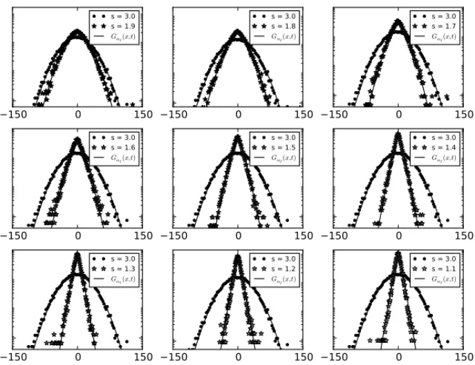
The second method to obtain the macroscopic parameters comprises the optimization fitting of the model solutionGα(x,t)(2.3) to the histogram of position of the processes according to the
subdiffusion. Hence,Gα(x,t)is fitted to subdiffusion processes to asses the parametersαand Dα. The adopted optimization method was the Broyden-Fletcher-Goldfarb-Shanno (BFGS) [5]
using a minimization function that considers the mean square error of the deviations. The param-eters obtained by that approach receive the subscriptT in mention to the theoretical solutions. Results of such analysis are depicted in Figure (3) and the parameters and mean squared devia-tions (MSD) are listed in Table (5).
Figure 3: Model solutionsGαT(x,t)(2.3) with parameters assessed by optimization fitting to the
histogram of positions generated by simulation over a timet ≥210of a CTRW for a population ofN=10.000 particles.
Table 1: Simulation data generated by power law PDFs for random jump sizes with r = 4 and for waiting time varyings in order to provide subdiffusion processes and the respective values of the parametersαandDα. The parameters assigned by ’S’ are
obtained by linear regression over the time evolution of the variance and those assigned by ’T’ are obtained by fitting the model solutionGα(x,t)(2.3) by BFGS optimization
technique. The mean squared deviations MSDs are also calculated in both cases.
s αS DαS αT DαT M D SS M D ST
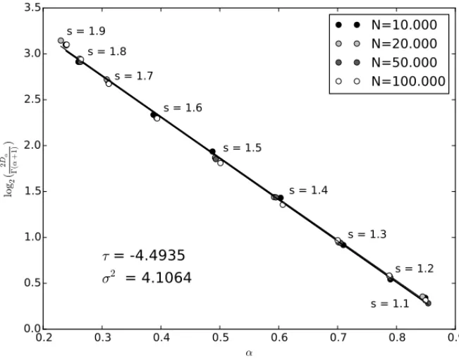
A calibration on the parameter space between simulation and theoretical model is depicted in (4) for varying populationN. The line slope is compatible with the effective values ofτ∗= −4.4935 andσ2=4.1064 in equation (2.4).
Figure 4: Calibration between microscopic or simulation parameters and macroscopic or theo-retical model parameters.
6 CONCLUSION
Both methods, in order to determine the parameters of the model, presented the same mean squared deviations. The method of the fitting dispersion by the time evolution of the variance, however, produces results with much lower computational cost and presents the same dispersion of the optimized fitting histograms of positions.
The definition of the power laws is not uniquely dependent of the power parameter p,(r,s), but it also demands the choose of two additional cutoffs; the firstεto avoid the singularity at zero and the upper limit cutoffto provide integrability when a given moment of interest (σ2,
τ) is divergent. In order to avoid excessive arbitrariness, we make a prescription which is to set a constraint between both cutoffs. Under such condition, the divergent factor of the moment of interest becomes near the unit.
parameters of the linear model written in terms of partial differential equations with fractional derivatives. However, not all cases of fractional derivatives in time were explored. We restricted ourselves to the case which have one of the derivatives being of integer order: the second order derivative in space was fixed and the time derivative remained fractional. Although we could generate a table with those values. We found a strong correlation between the values of the simulation parameters and those of the theoretical parameters.
RESUMO.Abordamos o problema da subdifus˜ao e da difus˜ao normal a fim de realizar uma
calibrac¸˜ao entre parˆametros simulados e parˆametros de um modelo subdifusivo. O modelo te ´orico consiste em uma equac¸˜ao de difus˜ao generalizada por derivadas fracion´arias
tempo-rais. Os dados s˜ao gerados por simulac¸˜oes baseadas em caminhadas aleat´orias de tempo
cont´ınuo com m´edia do tempo de espera e variˆancia do comprimento de saltos controlados para fornecer uma gama completa de casos entre a subdifus˜ao e a difus˜ao normal. A partir das
simulac¸˜oes comparamos a precis˜ao entre dois m´etodos para obter os parˆametros coeficiente de
difus˜ao e ordem da derivada fracion´aria: an´alise da dispers˜ao da variˆancia no tempo e ajuste por otimizac¸˜ao dos histogramas de posic¸˜oes com as soluc¸˜oes do modelo te ´orico. Destacamos
a conex˜ao entre os parˆametros das simulac¸˜oes e dos parˆametros do modelo te ´orico.
Palavras-chave:difus˜ao anˆomala, equac¸˜ao de difus˜ao fracion´aria, calibrac¸˜ao.
REFERENCES
[1] A.A.M. Arafa & S.Z. Rida. Exact solutions of fractional-order biological.Communications in Theo-retical Physics,6(2009), 992–996.
[2] O.P. Argrawal. Fractional variational calculus in terms of riesz fractional derivatives.J. Phys. A: Math. Theor.,40(2007), 6287–6303.
[3] J.G. Berryman. Evolution of a stable profile for a class of nonlinear diffusion equations with fixed boundaries.Journal of mathematical physics,18(1977), 2108–2115.
[4] M. Bologna, C. Tsallis & P. Grigolini. Anomalous diffusion associated with nonlinear frac-tional derivative fokker-planck-like equation: exact time-dependent solutions.Physical Review E,
62(2000), 2213.
[5] R.H. Byrd, P. Lu & J. Nocedal. A limited memory algorithm for bound constrained optimization. SIAM Journal on Scientific Computing,16(1995), 1190–1208.
[6] G. Combe, V. Richefeu, M. Stasiak & A.P.F. Atman. Experimental validation of a nonextensive scal-ing law in confined granular media.Phys. Rev. Lett.,115(2015), 238301.
[7] G.L. Eyink & H. Spohn. Negative-temperature states and large-scale, long-lived vortices in two-dimensional turbulence.Journal of statistical physics,70(1993), 833–886.
[8] G.A. Garosi, G. Bekefi & M. Schulz. Anomalous diffusion and resistivity of a turbulence, weakly ionized plasma.Appl. Phys. Lett.,15(1969), 334–337.
[10] H.J. Haubold, A.M. Mathai & R.K. Saxena. Mittag-leffler functions and their applications.Journal of Applied Mathematics,2011(2011), 51 pp.
[11] R. Hilfer, editor.Applications of fractional calculus in physics. World Scientific, (2000).
[12] V.M. Kenkre, E.W. Montroll & M.F. Shlesinger. Generalized master equations for continuous-times random walks.Journal of Statistical Physics,9(1973), 45–50.
[13] E.K. Lenzi, R.S. Mendes & C. Tsallis. Crossover in diffusion equation: Anomalous and normal behaviors.Physical Review E,67(3) (2003), p. 031104.
[14] F. Mainardi. Fractional relaxation-oscillation and fractional diffusion-wave phenomena.Chaos Soli-tons & Fractals,7(1996), 1461–1477.
[15] F. Mainardi. The fundamental solutions for the fractional diffusion-wave equations.Applied Mathe-matics Letters,9(6) (1996), 23–28.
[16] F. Mainardi.Fractional Calculus and Waves in Linear Viscoelasticity: An Introduction to Mathemat-ical Models. Imperial College Press, 2nd edition, (2010).
[17] R. Metzler & J. Klafter. The random walk’s guide to anomalous diffusion: A fractional dynamics approach.Physics Reports,339(2000), 1–77.
[18] R. Metzler & T.F. Nonnenmacher. Space- and time-fracitonal diffusion and wave equations, fractional fokker-planck equations, and physical motivation.Chemical Physics,284(2002), 67–90.
[19] E.W. Montroll & G.H. Weiss. Random walks on lattices II.J. Math. Phys.,6(1965), 167.
[20] Paolo Paradisi, Rita Cesari, F. Mainardi & Francesco Tampieri. The fractional fick’s law for non-local transport processes.Physica A: Statistical Mechanics and its Applications,293(2001), 130–142.
[21] I. Podlubny.Fractional Differential Equations. Academic Press, (1999).
[22] M.F. Shlesinger & J. Klafter. On the relationship among three theories of relaxation in disordered systems.Proceedings of the National Academy of Sciences,83(1986), 848–851.
[23] J. Stephenson. Some non-linear diffusion equations and fractal diffusion.Physica A,222 (1995), 234–247.
[24] L.T. Takahashi et al. Mathematical models for the aedes aegypti dispersal dynamics: travelling waves by wing and wind.Bulletin of Matematical Biology,67(2005), 509–528.
[25] C. Tsallis.Introduction to Nonextensive statistical mechanics. Springer, (2009).
[26] C. Tsallis & D.J. Bukman. Anomalous diffusion in the presence of external forces: Exact time-dependent solutions and their thermostatistical basis.Phys. Rev. E,54(1996), R2197.