DIET AND TROPHIC
POSITION OF DEEP-SEA
SHARKS IN THE
SOUTHWEST COAST OF
PORTUGAL
USING STABLE ISOTOPES ANALYSIS AND NUCLEIC ACIDS RATIOS (RNA/DNA)
DIET AND TROPHIC POSITION OF DEEP-SEA SHARKS IN
THE SOUTHWEST COAST OF PORTUGAL
USING STABLE ISOTOPES ANALYSIS AND NUCLEIC ACIDS RATIOS (RNA/DNA)
Master in Marine and Coastal Sciences
Work performed under the supervision of:
Advisor: Karim Erzini (CCMAR, UAlg)
Co-advisor: Ester Dias (CIIMAR, Porto)
i
DIET AND TROPHIC POSITION OF DEEP-SEA SHARKS IN
THE SOUTH-WEST COAST OF PORTUGAL
USING STABLE ISOTOPES ANALYSIS AND NUCLEIC ACIDS RATIOS (RNA/DNA)
“Declaro ser a autora deste trabalho, que é original e inédito. Autores e
trabalhos consultados estão devidamente citados no texto e constam da listagem
de referências incluída.”
"I declare to be the author of this work, which is original and unpublished.
Authors and works consulted are duly cited in the text and are included in the
list of references. "
_________________________________________ SOFIA GRAÇA ARANHA CARVALHO RAMOS
ii
“A Universidade do Algarve reserva para si o direito, em conformidade com o disposto no Código do Direito de Autor e dos Direitos Conexos, de arquivar, reproduzir e publicar a obra, independentemente do meio utilizado, bem como de a divulgar através de repositórios científicos e de admitir a sua cópia e distribuição para fins meramente educacionais ou de investigação e não comerciais, conquanto seja dado o devido crédito ao autor e editor respetivos”.
"The University of Algarve reserves the right, in accordance with the provisions of the Code of the Copyright Law and related rights, to file, reproduce and publish the work, regardless of the used mean, as well as to disseminate it through scientific repositories and to allow its copy and distribution for purely educational or research purposes and non-commercial purposes, although be given due credit to the respective author and publisher."
iii
“We but mirror the world. All the tendencies present in the outer world are to be found in the world of our body. If we could change ourselves, the tendencies in the world would also change. As a man changes his own nature, so does the attitude of the world change towards him. This is the divine mystery supreme. A wonderful thing it is and the source of our happiness. We need not wait to see what others do.”
iv
My journey throughout these past two years of my master has lead me to cross path with beautiful persons and circumstances. Staying apart from family and friends in such a defying situation in a foreign country it was a great challenge. I was lucky enough to have by my side my husband Tiago and my lovely loyal dog Snapper to whom I would like to thank at first place, since they have been with me 24/7 giving me love and strength to continue on the path of my dream, I am truly grateful for that. Also thank you Tiago for being on the field with me and helping me with the collection of the data, without your support I would not have strength to be onboard a commercial fishing vessel, love you to the moon and back! There are many people to whom I would like to acknowledge and to which without the support this work would not have been possible:
To my supervisor Prof. Dr. Karim Erzini at the University of Algarve which since the beginning believed on my work and decided to support this idea. Thank you for all the wise words and orientation and also for helping me surpass the obstacles that were faced throughout the time of the development of this study.
To my co-supervisor Dr. Ester Dias from University of Porto, a big thank you for you patient, collaboration and all the lessons learned on this challenging subject of stable isotopes. Thank you for your comprehension and companionship throughout the process and the dedicated time you spent to help me finish this work on time.
To my advisor Prof. Dr. Alexandra Teodósio to which despite her new position as vice-rector at the University of Algarve, never left me without support and was always very patient and dedicated to assist me. Thank you for teaching me this unexplored technique of RNA/DNA ratios on sharks and also for providing me the material necessary for all the analysis both at the laboratory and the field.
To prof Margarida Castro who borrowed me the temperature sensor and to all my colleagues from the “Fisheries Biodiversity and Conservation” and “ECOREACH” laboratories from the University of Algarve especially Vânia for helping me with the data acquisition for RNA/DNA ratios, Joana and ‘Camané’ for helping me gather the tools to be used both at the field and at the laboratory as for my laboratory colleagues Adella and Joffrey and Isidoro. Thank you as well to Paulo, the laboratory technician from CIMA and to Lilian Krug for the help with the hindcast temperature data from the Portuguese coast.
A big thank you to the fishermen onboard the commercial fishing vessel “Crustaceo” which helped with the collection of the data. Unfortunately, this kind of project is still only possible via deep-sea fisheries, and despite having too many disagreements with this activity, I still appreciate all the help provided and hope to make use of this data on the best way possible. I would like to thank all my professors from the master’s program and also the ones whom I cross path throughout my academic life, thank you for providing me the tools to improve my knowledge and skills.
Thank you for all my friends from the master program for providing a great atmosphere even inside and outside the classes, also for the great moments we have shared together, also for all the friends I have made over those two years of Portugal.
Nonetheless, a very special thank you to my family. Thank you for always be supportive and comprehensive on the hardest moments, also for the words of wisdom and encouragement which were crucial to shaping me into the person I am today.
v
lowest observed to date. Sharks are, in general, predators and thus crucial to maintain the balance of their direct and indirect preys. Due to their fragility and role in the marine food web, this study aimed at assessing the nutritional condition, diet, and trophic position (TP) of deep-sea sharks at the southwest coast of Portugal using for the first time a combination of two non-lethal approaches with deep-sea elasmobranchs: RNA/DNA (R/D) ratios, and stable isotope analysis (SIA). Muscle samples were collected from deep-sea shark species: Centrophorus squamosus, Centroselachus crepidater, Deania calcea, Deania profundorum, Etmopterus pusillus, Galeus atlanticus and Scymnodon ringens. Their potential prey were also collected and included, teleosts, crustacean and cephalopods. Overall, sharks presented a good nutritional condition indicating they have been feeding and that their diet might be supported by the species from the study area. The species with higher R/D values (e.g. G. atlanticus) are eating more frequently than species with lower ratios (e.g. D. profundorum). Sharks were divided in three groups according to SIA. The first group was composed by D. profundorum, E. pusillus, and G. atlanticus presenting low δ13C and δ15N values, indicating they were feeding on preys with low δ13C and δ15N values such as crustaceans and diel vertical migratory teleosts (group T3), presenting a TP range of 4.1-5.1. Second group of consumers is composed by S. ringens and C.squamosus with 13C and 15N-enriched values,
an indication they were feeding on preys with higher values of δ13C and δ15N such as migratory teleosts and cephalopods and presented a TP range of 5.6-6.1. The third group is composed by D.calcea and C.crepidater with a high isotopically variability suggesting intra-specific variation on the diet or a generalist behavior with the presence of a wider trophic niche and TP range of 5.1-6.3.
Keynotes: squaliformes; elasmobranchs; ecophysiology; eastern Atlantic Ocean; nutritional
vi
mais baixas observadas até o momento. Os tubarões são, em geral, predadores e, portanto, são cruciais para manter o equilíbrio do ambiente em que habitam. Devido à essa fragilidade e importância, este estudo teve como objetivo avaliar o estado nutricional, a dieta e a posição trófica (TP) de tubarões de profundidade na costa sudoeste de Portugal utilizando pela primeira vez uma combinação de duas abordagens não letais com elasmobrânquios de profundidade: Rácios de RNA/DNA e análise de isótopos estáveis (SIA). Amostras de músculos foram coletadas para tubarões - Centrophorus squamosus, Centroselachus crepidater, Deania calcea, Deania profundorum, Etmopterus pusillus, Galeus atlanticus e Scymnodon ringens e também para potenciais presas: teleósteos (dividos pelos seus valores de δ13C e δ15N nos grupos T1 à T4), crustáceos e cefalópodes. Em geral, os tubarões
apresentaram uma boa condição nutricional indicando que eles têm se alimentado e que sua dieta pode ser sustentada pelas presas da área de estudo. As espécies com maiores rácios de R/D (por exemplo, G. atlanticus) se alimentam mais frequentemente do que as espécies com menores rácios (por exemplo, D. profundorum). Os tubarões podem ser agrupados em três grandes grupos de consumidores de acordo com SIA. O primeiro é composto pelas espécies D. profundorum, E. pusillus e G. atlanticus com baixos valores de δ13C e δ15N indicando, portanto, uma dieta composta por presas com baixos valores de δ13C e δ15N como crustáceos
e espécies de teleósteos que realizam migração vertical diária, apresentando também uma variação de TP de 4,1 a 5,1 . O segundo grupo de consumidores é composto por S. ringens e C. squamosus que possuem valores enriquecidos de 13C e 15N, um indicativo de que eles se alimentam de presas com valores maiores de δ13C e δ15N como algumas espécies migratórias de teleósteos e cefalópodes e possuam uma variação de 5,6 a 6,1 de TP. O terceiro grupo é composto por D. calcea e C. crepidater onde apresentaram alta variabilidade isotópica sugerindo variação intraespecífica na dieta e/ou comportamento generalista com a presença de um nicho trófico mais amplo, e uma variação de TP 5,1 a 6,3.
Palavras-chave: squaliformes; elasmobrânquios; ecofisiologia; oceano atlântico leste;
vii
CHAPTER 1 ... 1
1. INTRODUCTION ... 2
Fishing the deep-sea ... 2
Deep-sea sharks ... 3
Nutritional condition, diet and trophic position of sharks ... 5
CHAPTER 2 ... 10
2. MATERIALS AND METHODS ... 11
2.1 Data Collection ... 11
2.2 RNA/DNA ratios (R/D) ... 14
2.3 Stable Isotopes Analysis (SIA) ... 15
CHAPTER 3 ... 19
3. RESULTS ... 20
3.1 Sharks and potential preys ... 20
3.2 Nutritional condition characterization ... 23
3.3 Food-web characterization ... 30
Identification and quantification of the main preys ... 30
CHAPTER 4 ... 39
4. DISCUSSION ... 41
4.1 Nutritional condition characterization ... 41
4.2 Trophic position ... 47 4.3 Limitations ... 49 CHAPTER 5 ... 51 5. CONCLUSION ... 53 6. REFERENCES ... 55 ANNEX A ... 74 ANNEX B ... 81
viii
the isobaths of sampling (Created with Mirone software). ... 11
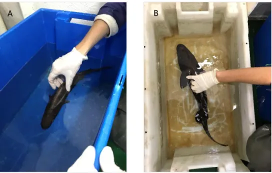
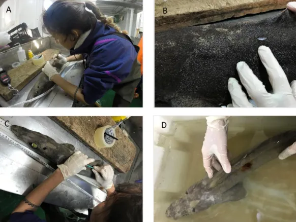
Figure 2.2: A EcloThermocronTM sensor; B led lure capsule ... 12 Figure 2.3: A, B Live sharks being handle inside the containers with sea water. ... 13 Figure 2.4: Muscle collection procedure and bandage for the live sharks. A Incision on the skin with
a scalpel; B, wound opened; C incision with the biopsy punch and D wound with bandage. ... 14
Figure 3.1: Taxa sampled in this study. The consumers (sharks) are Selachii and the sources include
the taxa Cephalopoda, Teleostei and Crustacea with its respective orders (excluding zooplankton copepods), families, species and individuals (n). ... 20
Figure 3.2: Number of adults and juvenile sharks collected in this study, according to gender (male
and female) The life stage of individuals from the S. ringens could not be determined (N/A). ... 22
Figure 3.3: European IUCN status of the sharks collected in the present study. LC, least concern;
DD, data deficient; NT, near threatened; EN, endangered. ... 23
Figure 3.4: Scatter plot of individuals standardized nucleic acid ratios (sRD) with the animal’s size.
Observed values in relation to the animal’s size (total length in cm), adjusted linear model (doted blue line). A RNA (mg); B DNA (mg); and C is the sRD. Cs, Centrophorus squamosus; Cc,
Centroselachus crepidater; Dc, Deania calcea; Dp, D.profundorum; Ep, Etmopterus pusillus; Ga, Galeus atlanticus and Sr, Scymnodon ringens. ... 25
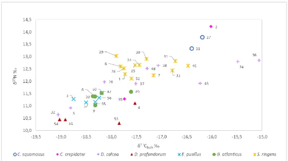
Figure 3.5: Linear regression between C:Nbulk and δ 13Cbulk(‰) for each shark species. ... 26 Figure 3.6: Sharks' δ13C and δ15N values . Numbers corresponds to the code of each individual which
can be found in the Table 0.3 in ANNEX A. ... 28
Figure 3.7: Boxplot with the isotopic ratios from all shark species. The horizontal black line inside
the boxplot is the medium value, the standard deviation is represented by a vertical black line and inside the green bloxpot the minimum quartile is 25% and maximum quartile of 75%. A, δ13C (‰)
and B, δ15N (‰). Cs, Centrophorus squamosus; Cc, Centroselachus crepidater; Dc, Deania calcea;
Dp, D.profundorum; Ep, Etmopterus pusillus; Ga, Galeus atlanticus and Sr, Scymnodon ringens. 30
Figure 3.8: Potential preys average (±SD) δ13C and δ15N values for each species addressed by a code
(check Table 0.2 from the ANNEX A). Teleosts (yellow triangles); crustacean (blue squares) and cephalopods (green diamond). ... 31
Figure 3.9: Cluster analysis of the potential sources of the deep-sea sharks from the SW coast of
Portugal. Species names for the codes addressed here, can be found in the Table 0.2 ANNEX A . 31
Figure 3.10: Average (± SD) δ15N and δ13C values of the main groups of sharks potential prey (T1,
T2, T3, T4 for teleosts, Cr for crustaceans, and Cf for cephalopods) and individual sharks δ15N and
δ13C values without corrected trophic fractionation. Cs, Centrophorus squamosus; Cc,
Centroselachus crepidater; Dc, Deania calcea; Dp, D.profundorum; Ep, Etmopterus pusillus; Ga, Galeus atlanticus and Sr, Scymnodon ringens. ... 33
Figure 3.11: Proportion of each group of prey to the consumers biomass. Boxplot with the lowest to
the highest density region (95%). T2 and T3 are groups of Teleostei; Cr is the contribution of the Crustacea and Cf is Cephalopoda (squids and octopus combined). ... 35
Figure 3.12: Corrected standard ellipse areas (SEAc) and overlap between shark species. ... 36 Figure 3.13: Trophic position of consumers and potential sources groups with standard deviation of
each group. Cs, Centrophorus squamosus; Cca-j, Centroselachus crepidater adult and juvenile; Dc,
Deania calcea; Dp, D.profundorum; Ep, Etmopterus pusillus; Ga, Galeus atlanticus and Sr, Scymnodon ringens. T1-T4 are groups of teleosts; Cr, are crustaceans and Cf, are cephalopods. .. 38
ix
Figure 0.3: Teleosts from group T2 with migratory behavior, collected from the bathyal zone in the
southwest coast of Portugal. ... 82
Figure 0.4: Teleosts from the group T3 with species that performs diel migratory migrations and
presents lower values of δ15N , from the bathyal zone in the southwest coast of Portugal. ... 83 Figure 0.5: Teleosts from the group T4 with average values of δ15N from the bathyal zone in the
southwest coast of Portugal. ... 84
Figure 0.6: Crustaceans collected from the bathyal zone in the southwest coast of Portugal. Species
with * are the target of this crustacean bottom trawler. ... 85
Figure 0.7: Cephalopods collected from the bathyal zone of the southwest coast of Portugal. ... 86 Table 3.1: Shark species with number of individuals (n), average (±SD) total length (TL, cm) and
weight (g); gender (male or female); number of adults (A) and juveniles (J) and unknown life history (N/A); condition of the individuals: good (G), poor (P) and dead (D) is also presented. ... 22
Table 3.2: Species size (average ± SD), average values for RNA and DNA given in mg also, average
(±SD) for sRD. ... 23
Table 3.3: Number of individuals sampled from each shark species, average and standard deviation
of isotopic values of δ15N (‰) and δ13C
bulk(‰) of the sharks’ species. δ13Cbulk(‰) is the ratio before
lipid correction and δ13C
ptn(‰) is the ratio after mathematical lipid correction...27 Table 3.4: Results of PERMANOVA test for differences of δ13C and δ15N values between different
shark species. Cs Centrophorus squamosus; Dc Deania calcea; Dp Deania profundorum; Ep
Etmopterus pusillus; Ga Galeus atlanticus; Sr Scymnodon ringens. * species significantly different
p < 0.05 ... 29
Table 3.5: Group of sources and constituent species. T1, T2, T3 and T4 are groups of Teleostei; Cr
stands for Crustacea and Cf stands for Cephalopoda with average (±SD) of δ13C and δ15N values of
each group. The species code can be found in Table 0.4, ANNEX A. ... 32
Table 3.6: Results from corrected standard area (SEAc ‰2) total area (TA) and niche overlap (‰)
between the species Dc, Deania calcea; Dp, Deania profundorum; Ep, Etmopterus pusillus, Ga,
Galeus atlanticus and Sr, Scymnodon ringens. ... 37
Table 3.7: Trophic position of shark species, average values (± SD) for each species. ... 37 Table 0.1: Classification of the taxa sampled with the respective order, family, species (whenever
possible) and number of individuals of each species (n). ... 74
Table 0.2: Taxa of each source species and the code used. ... 76 Table 0.3: Complete list of parameters from each individual of the consumers species. Centrophorus
squamosus; Centroscelachus crepidater; Deania calcea, D.profundorum; Etmopterus pusillus, Galeus atlanticus and Scymnodon ringens. Individual species field code. Sex M, male or F female.
TL total length in cm. Life Stage A, adult; J, juvenile or N/A unknown. Condition G, good; P, poor and D, dead. δ15N and δ13C in parts per mil (‰). sRD is the standardized RNA/DNA ratios. ... 77 Table 0.4: Complete list of sources individuals containing the species field code, length in cm (either
total length for teleosts, carapace length for crustaceans and mantle length for cephalopods); the weight in grams, Nitrogen and Carbon values (%); δ15N and δ13Cvalues from the bulk and after lipid
correction (δ13C
x
não suportam altos níveis de exploração devido às características do seu ciclo de vida que incluem extrema longevidade, baixa taxa de crescimento, maturação tardia e baixa fecundidade. Os elasmobrânquios de profundidade são ainda menos resistentes à exploração e a sua produtividade está entre as mais baixas observadas até o momento, entre os organismos de profundidade. Embora o seu papel varie entre espécies e regiões, os tubarões são geralmente aceites como predadores nas cadeias alimentares marinhas, sendo de extrema importância para a manutenção do equilíbrio de todo o ecossistema através da ligações tróficas que estabelecem. Sendo assim, é crucial a avaliação das suas características ecofisiológicas e biológicas por meio de abordagens não-letais, a fim de compreender a sua vulnerabilidade e o seu papel dentro de ecossistemas específicos. Os ácidos nucleicos como os rácios de RNA/DNA (R/D) são ferramentas importantes porque fornecem uma medida de curto prazo das condições ecofisiológicas dos animais (por exemplo, 1-3 dias), embora nunca tenham sido aplicados em estudos com elasmobrânquios de águas profundas. A análise de isótopos estáveis (SIA) é uma ferramenta muito útil para estudar não só as interações tróficas em cadeias alimentares aquáticas, mas também inferir o uso do habitat e os padrões de movimento de indivíduos e populações. Ambas as metodologias podem ser usadas como uma abordagem não letal para o estudo de animais frágeis e únicos, como os tubarões. Como informações sobre organismos de profundidade são ainda muito escassas (especialmente no caso de tubarões), o objetivo principal do presente estudo foi contribuir para aumentar o conhecimento existente sobre o estado nutricional, a dieta e a posição trófica dos tubarões de profundidade da costa sudoeste de Portugal combinando pela primeira vez rácios de R/D e SIA em tubarões.
Para este fim, foi realizada uma campanha de amostragema em Fevereiro de 2018, durante três dias, a bordo de um barco de pesca de arrasto de fundo para captura comercial de crustáceos. As recolhas foram feitas entre 1.107 e 1.350 m de profundidade e amostras musculares das espécies de tubarões e suas potenciais presas foram recolhidas para análise. Os tubarões encontrados na área foram o lixa Centrophorus squamosus (n=2); sapata preta Centroselachus crepidater (n=2); sapata Deania calcea (n=9), sapa branca D. profundorum (n=4) xarinha preta Etmopterus pusillus (n=5); Galeus atlanticus (n=5) e o arreganhada Scymnodon ringens (n =12). As potenciais presas incluíram teleósteos dividos em grupos i.e. T1 com elevado δ15N e composto por espécies não-migratórias, T2 com espécies migratórias, T3 com espécies com baixos valores de δ15N que realizam migrações verticais
diárias e T4 com valores médios de δ15N incluindo, crustáceos (caranguejos, camarões e lagostas) e cefalópodes (lulas e polvos). Fêmeas representaram a maioria dos tubarões capturados (69%). Foram apanhados mais juvenis (36%) do que adultos (33%), embora para S.ringens (31%) não haja informação suficiente, para fazer esta classificação. No geral, os tubarões apresentaram uma boa condição nutricional dado a média dos rácios estandarditizados de R/D foi superior a 0. Isso indica que eles se alimentaram no últimos 1-3 dias, e também, que talvez a sua dieta seja sustentada pelas espécies da área de estudo. Espécies que apresentaram rácios mais elevados, como o G.atlanticus (0,63) indicam que
xi
Os resultados do modelo de mistura de isótopos estáveis (95 % CI) indicam que os crustáceos foram os principais contribuintes (3-78%) para a biomassa de D. calcea, seguidos pelos teleósteos do grupo T2 (0-65%). Por outro lado, D. profundorum apresentou uma dieta de contribuições iguais dos dois grupos de teleósteos T2 e T3, crustáceos e cefalópodes, bati- demersais e pelágicos. Etmopterus pusillus exibiu uma preferência de T3 (21-83%), o que reforça a ideia que E. pusillus também podem realizar migrações diárias verticais para se alimentar. O Galeus atlanticus apresentou maior contribuição do grupo de teleósteos T3 (11-69%), seguido pelos crustáceos (05-60%). A espécie Scymnodon ringens foi a única com uma preferência maior por um grupo específico, neste caso os crustáceos (46-89%) e, por apresentar um nicho trófico mais pequeno, pode indicar que poderá ser ser um predador mais seletivo. Algumas espécies, como D. profundorum, E. pusillus e G. atlanticus, apresentaram valores demasiado baixos de δ15N, quando comparados com os das presas potenciais
capturadas. Isto poderá indicar que nem todas as presas relevantes para a dieta dessas espécies foram amostradas neste estudo,e que poderão incluir mictofídeos e eufasiáceos. As fêmeas juvenis de D. calcea e D. profundorum mostraram a maior amplitude de nicho o que pode indicar que elas são predadores generalistas. Os indivíduos da espécie D. calcea parece estar a alimentar-se mais frequentemente do que D.profundorum devido ao fato de que D.profundorum apresentou menores rácios de R/D em comparação com D.calcea e outras espécies de tubarões.
De uma forma geral, as espécies de tubarões foram as que apresentaram a maior posição trófica (TP 4,8 a 6,3), seguidos pelos teleósteos (TP 4,0 a 5,0), cefalópodes (TP 3,8 a 4,4) e crustáceos (TP 3,4 a 4,1).
Apesar de este estudo apresentar algumas limitações, como em relação ao número de amostras e tecidos analisados, os resultados aqui obtidos são, em geral, satisfatórios para a interpretação dos principais objetivos inicialmente propostos. Novos estudos são necessários a fim de fornecer uma informação mais detalhada do estado nutricional, composição da dieta e maior resolução trófica dos tubarões de profundidade. Para isso, é aconselhável o uso de diferentes tecidos para a realização de SIA - uma vez que os tecidos assimilam a proteína ingerida em tempos diferentes ‘turnover’ (dias, anos e até décadas) - juntamente com um maior período de coleta de dados para caracterizar a sazonalidade da dieta; o uso de diferentes fatores de enriquecimento trófico para diferentes tipos de organismos; uma boa escolha do organismo de base que tem que estar de acordo com a cadeia trófica em estudo; um número maior de indivíduos para avaliar mudanças da dieta ao longo do desenvolvimento e entre géneros; amostragem em diferentes limites batimétricos, pois acredita-se que algumas espécies agregam por tamanho e sexo em diferentes profundidades; finalmente, o uso de diferentes tipos de ferramentas para amostrar diferentes grupos de presas.
1
CHAPTER 1
2
1. INTRODUCTION
Fishing the deep-sea
Continental shelf break is located at approximately 200 m depth and function as the boundary between 'shallow' and 'deep sea', i.e. everything below 200 m depth is considered the deep-sea realm and it covers more of the Earth’s surface than any other habitat (Gage and Tyler 1991). The bathyal zone extends from a depth of 1,000 to 4,000 m below the ocean surface. At this zone, physicochemical parameters such as temperature and salinity reach constant values. Because of its constant darkness it is also called the “midnight zone” and the only light coming from those depths, and below it, results from animal bioluminescence (NOAA 2017).
The deep-sea was believed to be a depauperated ecosystem due to its high pressures with an average of 400 atm, low temperatures with a mean of 4° C and little to no light penetration (Rowe 1983). However, today it is among the biomes with the highest biodiversity on Earth (Hessler and Sanders 1967; Grassle and Maciolek 1992; Snelgrove and Smith 2002). Still, little is known about these habitats due to its remoteness and difficulty in sampling at great depths (Snelgrove and Grassle 2001). Some commercially important species are known to inhabit deep-sea areas, e.g. the redfish (Sebastess spp.); the orange roughy (Hoplostethus atlanticus) (Norse et al. 2012) as well as some crustacean species such as the giant red shrimp (Aristaeomorpha foliaceae) and the scarlet shrimp (Aristaeopsis edwardsiana) (Figueiredo et al. 2001).
Despite the apparent higher levels of productivity over seamounts and similar features (Koslow et al. 2000) species in the deep-sea cannot support high levels of exploitation due to their life-history characteristics which includes extreme longevity, slow growth rate, late maturity, and low fecundity (Koslow et al. 2000; Morato et al. 2006; Norse et al. 2012). Thus, stock depletion is more rapid and recovery is consistently much slower than for species in shallow waters (Roberts 2002).
Commercial marine fishing has been occurring at increasing depths around the globe since 1970 which coincided with the collapse of shallow water stocks (Roberts 2002; Morato et al. 2006). The need to fish at higher depths stimulated the development of new and robust fishing gear; nonetheless, the access to deep-sea habitats it is still difficult because it requires expensive equipment and rigorous logistical protocols, and its success depends upon regional- or local-scale production processes. It seems likely that deep-sea fishing can only be profitable if pursued in the present mode of serial depletion (Roberts 2002). Thus, the need for site-specific
3
information and a precautionary approach is required as the footprint of fisheries expands (Norse et al. 2012; Brooks et al. 2015).
The fishing sustainability of some deep-sea species is related to (a) the ability of these species to also inhabit systems shallower than 200 m; (b) relatively high population resilience, and (c) the use of low-tech, non-trawl methods. Therefore, bottom trawling fisheries are not sustainable for any deep-sea species (Merrett and Haedrich 1997; Norse et al. 2012).
Bottom trawling fisheries pressure at the Portuguese continental waters is high (ICES Sub-area IXa). Over 100 trawlers using cod-ended mesh sizes, ranging from 55 to 70 mm, fish a large number of species (Campos et al. 2007). For the years 2012 to 2014 crustacean bottom trawlers landed 3.481 tons of catch and the most representative species were the rose shrimp (Parapenaeus longirostris) accounting for 44% of the total catch, followed by Nephrops norvegicus (12%), Merluccius merluccius (10%), and Octopus vulgaris (9%) (Bueno-Pardo et al. 2017). The seabed integrity indices for bottom-trawling fisheries in Portuguese waters are among the lowest of all Europe, and this is the result of a large footprint per unit of landing (ca. 17 km²/t) and of a large total area (93.6%) where the trawling takes place (Eigaard et al. 2017) highlighting the intense pressure on deep-sea benthic habitats by bottom trawler fisheries.
Deep-sea sharks
Sharks are one of the most abundant and diverse groups of consumers in the ocean being found throughout the world’s oceans – from coastal waters to the open ocean, from the surface to depths of 3,000 m (Priede et al. 2006) and presenting all the reproductive traits from vertebrates, from egg laying to placental viviparity (Cahmi 2008). They also have a variety of feeding habits, preying upon smaller sharks, marine mammals, teleosts, crustaceans, and zooplankton. Although their role in the marine food webs varies between species and regions, they are generally accepted as predators (Cortes 1999; Simpfendorfer and Dulvy 2017). As such, they are extremely important for the entire ecosystems balance, by regulating not only their direct main preys, but also second and third degree non-prey species through trophic linkages (Schindler et al. 2002).
Chondrichthyans (sharks, rays and chimeras) are among the most vulnerable taxa due to their extremely conservative K-selected life history strategy (i.e. slow growing, late to mature, small number of descendants) (Cortes 1999) and thus, are characterized by slow population turnover rates which makes them especially vulnerable to fisheries. Deep-sea chondrichthyans are overall less resilient to fisheries pressures than coastal and epipelagic species due to parameters such as high pressures and low temperatures which are known to slow down the metabolism of
4
the animal, directly affecting the growth rates (Vetter and Lynn 1997; Gordon 2001) and because of that, their productivity is amongst the lowest observed to date (Simpfendorfer and Kyne 2009). In these animals, overexploitation can occur even with low levels of fishing mortality and once they start to decline, it can take decades for populations to recover (Anderson 1990; Stevens et al. 2000; Pauly 1980; McCann and Shuter 1997; Gordon 1999),
Some of the world’s elasmobranch (sharks and rays) populations are in rapid decline, and present a high potential risk of extinction in the future (García et al. 2008). However, almost half have insufficient data to support any form of assessment (Heupel and Simpfendorfer 2010). In Europe, according to the European Red List of Marine Fishes (IUCN, Nieto et al. 2015) the most threatened taxa is the Chondrichthyes comprising 40.4% of the endangered European marine species, while elasmobranchs represent 100% (n = 15) of ‘critically endangered’ (CR) species. The most relevant threat to marine fishes is the over-exploitation of both targeted and non-targeted species, more specifically, several deep-sea elasmobranch populations observed catastrophic declines in recent years, e.g. the picked dogfish, Squalus acanthias (Linnaeus, 1758) had its northeastern population depleted to about 5% of the original biomass (Hammond and Ellis 2004); the blue skate, Dipturus batis (Linnaeus, 1758) went locally extinct in the Mediterranean (Abdulla 2004). This is of great relevance taking into account that deep-sea chondrichthyans comprise approximately half (47.6%) of extant taxa (Cotton and Grubbs 2015). Thus, the lack of information raises concerns over the health of deep-sea chondrichthyan populations and creates uncertainty regarding potential effects of their removal on deep-sea ecosystem structure and function, since for tropical communities it was proved that the removal of sharks affected the condition and abundance of other fishes, across many trophic levels (Stevens 2000; Cox et al. 2002). For example, the seasonal presence of tiger sharks (Galeocerdo cuvier) in Shark Bay, Australia, was found to limit the habitat use and abundance of dolphins and dugongs in productive shallow areas (Heithaus and Dill 2002; Heithaus et al. 2006; Wirsing et al. 2007). More recently, Hammerschlag et al., (2018) found that shark declines at unprotected coral reefs in western Australia can induce physical changes in some reef fishes (e.g. smaller fins and eyes) in comparison to areas where shark populations are healthy. Similarly to other regions in the world, the distribution of elasmobranch species along Portuguese waters is poorly known (Albuquerque 1956; Figueiredo et al. 1996). At the south coast of Algarve (S- Portugal) sixty species of sharks were identified, including several deep-sea species such as the smooth lantern shark (Etmopterus pusillus), knifetooth dogfish (Scymnodon ringens), the birdbeak dogfish (Deania calcea), arrowhead dogfish (D. profundorum), leafscale gulper shark (Centrophorus squamosus) and the longnose velvet
5
dogfish (Centroselachus crepidater) which are commonly caught as bycatch of longline and crustacean trawlers fisheries (Borges et al. 2001; Coelho and Erzini 2008; Leitão et al. 2014). The great majority of deep-sea sharks including those from the families Scyliorhinidae and Etmopteridae, have little or no commercial value and therefore are frequently discarded (Monteiro et al. 2001; Coelho and Erzini 2008).
Decreases in the abundance of apex or meso-predators such as sharks may cause alterations in ecosystems through competitive release (i.e. without its predator, the immediate prey would increase its number and thus decrease the numbers of their direct preys), which would therefore, alter fish population dynamics (Stevens 2000). Thus, the understanding of the trophic ecology of sharks is of extreme importance to evaluate the possible consequences of their stock’s reduction. Given the role of sharks in the marine ecosystems and due to their increasing vulnerability to overfishing and habitat degradation (Ferretti et al. 2010; Worm et al. 2013) they became the focus of several marine conservation studies which aim at understanding their ecology and behavior in order to develop effective management and conservation strategies (Simpfendorfer et al. 2011; Molina et al. 2012; Jordan et al. 2013; Kynoch et al. 2015).
Nutritional condition, diet and trophic position of sharks
Condition and growth of organisms can be estimated with biochemical techniques, and to date, the most widely-used index is the bulk ribonucleic acids (RNA) and deoxyribonucleic acids (DNA) analysis (RNA/DNA). The RNA/DNA (R/D) is able to provide a short-term measure of ecophysiological conditions (i.e., past 1–3 days) (Buckley et al. 1999), based on the concept that DNA concentrations within individual cells remain fairly constant while RNA concentrations increase as protein synthesis increases and varies with age, life-stage, organism size, disease-state and with changing environmental conditions (Bulow 1970; Buckley 1980; Ferron and Leggett 1994; Suthers et al. 1996). Thus, a recently well-fed, metabolically active growing individual, should have a relatively high R/D compared to a starving, metabolically inactive individual (Bulow 1987; Robinson and Ware 1988; Richard et al. 1991).
For about fifty years, nucleic acid ratios have been used as a biochemical indicator of the physiological and nutritional state of aquatic organisms in natural environment (Holm-hansen et al. 1968). R/D is a macromolecular index frequently used as an indicator of protein synthesis and is considered a reliable indicator of instantaneous condition and growth (Rooker et al. 1997; Okumura et al. 2002; Islam and Tanaka 2005; Vidal et al. 2006). To date, a number of studies in ecology, toxicology, aquaculture and fisheries have used this approach to assess the condition of different organisms, mainly plankton (Sutcliffe 1965; Holm-Hansen et al. 1968; Dortch et
6
al. 1983; Berdalet and Dortch 1991; Gorokhova and Kyle 2002; Cruz et al. 2017), larval fish (Buckley 1984; Bulow 1987; Caldarone et al. 2003; Chícharo et al. 2003; Garcia et al. 2003; Caldarone 2005; Buckley et al. 2008), bivalves (Wright and Hetzel 1985; Chícharo and Chícharo 1995; Dahlhoff and Menge 1996; Chícharo et al. 2001), cephalopods (Clarke et al. 1990; Sykes et al. 2004; Vidal et al. 2006), crustaceans (Grémare and Vétion 1994; Lemos et al. 2002; Chícharo et al. 2007) and vertebrates like sea turtles (Roark et al. 2009; Vieira et al. 2014), juvenile and adult fishes (Bulow 1970; Thorpe et al. 1982; Carter et al. 1998; Buckley et al. 1999; Smith and Buckley 2003; Islam and Tanaka 2005; Mercaldo-Allen et al. 2006; Caldarone et al. 2006; Chícharo et al. 2007; Vinagre et al. 2008a).
Although the R/D approach has been widely used on many different marine organisms, including vertebrates, only one published study applied this tool on sharks. Tavares et al. (2006) analyzed the physiological condition of juveniles of smooth dogfish shark (Mustelus canis) at the northern coast of Venezuela using R/D ratios. No studies on deep-sea sharks were found. The fact that samples from deep-sea species are not easy to obtain (Brooks et al. 2015), biological and ecological studies on deep-sea sharks, especially for the Portuguese coast are very scarce. Nonetheless, it is possible to find studies on deep-sea sharks’ diet based on stomach content analysis (Costa 1998; Santos and Borges 2001; Coelho and Erzini 2007, 2008; Xavier et al. 2012; Coelho et al. 2015; Muñoz 2015; Gamito et al. 2016) which is the most commonly used method to analyze the diet and estimate trophic position of consumers in the aquatic food web. Perhaps, the most important study on sharks’ diet and trophic position is that of Cortés (1999) where the author showed, based on stomach content analysis of more than 149 shark species, that sharks are top predators being predominantly tertiary consumers (trophic level TL > 4) consuming a wide range of secondary consumers, i.e. carnivorous preys with a trophic level of 3.
Stomach content analysis provides detailed information on the food sources consumed at a given time. However, it does not provide information on the food sources which are assimilated by the consumer and in most cases requires the death of the animal. Also, stomach content analysis can be biased due to the presence of unrecognized prey items, loss of prey by regurgitation induced by stress with handling, among others (Vander Zanden et al. 1997; Pinnegar and Polunin 1999; Pinnegar et al. 2001; Renones et al. 2002). Deep-sea teleosts and elasmobranchs often regurgitate food as they are brought to the surface (Bowman 1986) and prey items from deep-sea communities often are fragile and difficult to identify (Cailliet et al. 1999; Drazen et al. 2001; Robinson et al. 2007).
7
Over the past decades, stable isotope analysis (SIA) has emerged as a useful biochemical tool in ecological research to study trophic interactions in aquatic food webs and also to infer habitat use and movement patterns of individuals and populations (Hobson 1999; Hussey et al. 2012; Layman et al. 2012). The analysis of stable isotopes, in particular of nitrogen (δ15N: 15N/14N) and carbon (δ13C: 13C/12C), is a useful method to clarify the structure and dynamics of aquatic
food webs. The δ15N values are usually used to determine the trophic level of a certain consumer
while the δ13C values are useful indicators of the origin of the food sources assimilated by
consumers (Polunin et al. 2001). This technique is based on the relationship between the isotopic composition of the organic matter (OM) in the ecosystem and the isotopic composition of the consumer’s tissues that incorporate this OM into their structural components and energy reserves (Peterson and Fry 1987). Thus, the stable isotope ratio of a consumer reflects its diet, demonstrating an average trophic fractionation (i.e., the difference between the consumer and its diet) of + 0.4 for δ13C and + 3.4 for δ15N per trophic level (Post et al. 2004). The trophic fractionation may vary according with the consumer’s nutritional status (Hobson et al., 1993) lipid content, quality of the diet, ontogeny, size, age, and with the type of tissue analyzed (Minagawa and Wada 1984; Zanden and Rasmussen 2001; Post 2002; Caut et al. 2008; Caut et al. 2010).
A series of improved quantitative approaches for analyzing stable isotopes over the past decade contributed to the improved understanding of food webs, for example, providing new insight into food-chain length (Post 2000), elucidating trophic relations in aquatic food-webs (Vander-Zanden et al. 1997; Post 2002) niche variation (Moore and Semmens 2008; Martínez Del Rio et al. 2009; Semmens et al. 2009; Votier et al. 2010) and human-driven shifts in community structure (Layman et al. 2007; Schmidt et al. 2007).
For large highly mobile animals inhabiting environments where they are difficult to observe, SIA is a useful tool and has been applied in shark ecology studies (Shiffman et al. 2012; Shipley et al. 2017), providing information on trophic structure (Estrada et al. 2003; Layman et al. 2007; Hussey et al. 2014, 2015; Churchill et al. 2015b), resource use (Matich et al. 2011, 2017; Heithaus 2013), diet ontogenetic shifts (Estrada et al. 2006; Madigan et al. 2015a), and movement patterns (Carlisle et al. 2012; Munroe et al. 2015).
Stable isotopes analysis (SIA) in elasmobranch may target different tissues including muscle, whole blood, red blood cells, cartilage, plasma, and liver (Hussey et al. 2012). The choice of a certain tissue will depend on the temporal resolution of interest (Pinnegar and Polunin 1999). For instance in sharks, the plasma, muscle, and cartilage will reflect feeding behaviors from the previous months, years, and decades, respectively (MacNeil et al. 2005; Caut et al. 2009; Kim
8
et al. 2012a). White muscle provide long-term dietary estimation due to its slower turnover rates in comparison to blood or liver, which exhibit high metabolic activity and thus, provides information of the diet for the previous months (Pinnegar and Polunin 1999; Estrada et al. 2006; l et al. 2015b). White muscle it is one of the most commonly sampled tissues because it can be non-lethal and can be sampled from multiple individuals of different size, sex or maturity to provide an integrated view of a species over ontogeny (Papastamatiou et al. 2010; Abrantes and Barnett 2011; Hussey et al. 2011, 2012).
SIA is also becoming increasingly applied in deep-sea systems (Polunin et al. 2001; Pethybridge et al. 2012; Churchill et al. 2015b; Shipley et al. 2017), because it allows to quantify ecologically significant community interactions, unique to deep-sea systems. For instance, trophic interactions among deep-sea sharks in the Gulf of Mexico allowed to understand that the stable isotopes varied as a matter of regions, ontogenic factors, time and gender (Churchill et al. 2015b); Pethybridge et al. (2012) correlated the biomagnification of total mercury levels (THg) in the deep-sea community of Southeastern Australia, with physical-chemical (bathome affinity) and community structure (presumably species composition and food chain length), and more recently Preciado et al. (2017) pointed out that the values of trophic position (TP) from SIA were significantly higher than the values from stomach content analysis for a seamount benthic community of deep-sea fishes on the northeast Atlantic. In Portugal, SIA has been applied in ecological studies since the year 1984, in studies on food web dynamics involving teleosts (Vinagre et al. 2008b; França et al. 2011; Vinagre et al. 2011, 2012, 2015; Colaço et al. 2013; Farias et al. 2014; Rossi et al. 2015; Dias et al., 2017). For deep-sea fauna, only a few studies were carried out off the eastern coast of Portugal along with the islands of Azores and Madeira (Correia et al. 2011; Colaço et al. 2013; Farias et al. 2014). Nothing was found in the literature on SIA studies of elasmobranchs or of deep-sea fauna off the southern coast of Portugal. This is relevant because it shows that there is a lack of data for SIA on deep-sea species for Portugal in general and especially for elasmobranchs.
In addition, SIA in elasmobranchs have never been associated to an indicator of nutritional and health state such as the RNA:DNA ratio. This is relevant because in order to study trophic position and dietary composition of marine organisms, it is important to assure that the sampled organisms have been feeding in the area and this can be assessed by condition and growth indicators, without the need of killing fragile and endangered animals such as sharks to conduct stomach content analysis, since only a very small portion of muscle is necessary to conduct the analysis.
9
Therefore, this study aims at assessing the ecophysiological condition, diet and trophic position of deep-sea sharks from the southern-west coast of Portugal combining non-lethal approaches. R/D analysis was performed to evaluate the ecophysiological condition while carbon (δ13C:
13C/12C) and nitrogen (δ15N: 15N/14N) stable isotope analysis (SIA) were used to access dietary
and trophic position information. Specifically, the aims of this study were to: • Assess the nutritional condition of sharks using R/D ratios;
• Identify the main preys and quantify its importance to sharks’ biomass using SIA; • Determine the trophic niche overlap between shark species;
• Determine the sharks’ trophic position.
This was done with the intention to contribute to fill the extant gap and improve the knowledge on the deep-sea sharks from the southwest coast of Portugal.
10
CHAPTER 2
11
2. MATERIALS AND METHODS
2.1 Data Collection
The Portuguese coast provides a great variety of marine and coastal habitats being located in a biogeographic transition zone between subtropical and temperate waters allowing an overlap of species limits between the northern and southern regions (Cardoso et al. 2019). This coast is also characterized by specific hydrographical features such as the presence of a relative warm and salty water at intermediate depths (∼1000 m), resulting from the mixing between the Atlantic Intermediate Water and the Mediterranean Water (MW) flowing through the Strait of Gibraltar (Ambar 1982).
One field sampling of three days was conducted in February 2018 on board of a crustacean bottom trawler off the southwest coast of Portugal, which targets the giant red shrimp (Aristaeomorpha foliacea) and the scarlet shrimp (Aristaeopsis edwardsiana) leaving from the fisheries port of Sines, Portugal. Sampling took place between 38°07.12 N / 9°23.09 W and 37°51.19 N / 9° 33.058 W (Figure 2.1).
Figure 2.1: Study area at the southern-west coast of Portugal presenting the fishing port of Sines and the isobaths of sampling (Created with Mirone software).
Sharks and its potential prey were sampled using a 90 m- bottom trawl (with a meshsize of 70 mm in the codend) towed for 4 h at a velocity varying from 2.1 to 2.7 knots. Six hauls were
12
performed in these conditions at depths varying between 1107 and 1350 m although the data was collected from only five hauls, due to the absence of organisms of interest for this study from the haul # 4. The temperature sensor EcloThermocronTM series 415BC904000000F3 was placed inside a led lure capsule (Figure 2.2), which is used for the squid fisheries, and was attached to the mouth of the net on the inner upper side. This lure capsule is known to resist pressures around depths of 400 m and therefore the temperature was only recorded for the first two hauls (for each 5 minutes).
Figure 2.2: A EcloThermocronTM sensor; B led lure capsule
While the target species were being selected by the fishermen, the live sharks were selected among the by-catch species and placed inside two large containers filled with sea water (Figure 2.3). Based on a rapid external observation, sharks were analyzed following the order: 1) in good condition 2) in poor condition, and 3) dead sharks (that died during the tows). These three categories were chosen according to previous studies (Benoît et al. 2010; Braccini et al. 2012; Rodríguez-Cabello and Sánchez 2017) where:
• Good condition: strong movements and lively swimming;
• Poor condition: spiracles movement, floats in the container with water, no body movement; • Dead: no response
Each individual was measured (total length -TL: from the tip of the snout to the tip of de caudal fin (cm) - in order to assess the life stage (adult or juvenile), weighted (g), sexed and identified onboard, or photographed for later identification whenever it was not possible to identify it immediately. Sharks were identified following the field book of Compagno et al. (2005). Their vulnerability was assessed through the European Union (EU) list of deep-water sharks (EU Regulation, No: 1182/2013) which have a zero total allowance catch (TAC) of some of the
13
sea shark species, and also by the European Red List from the International Union of Conservation of Nature IUCN (EU 2013; Nieto et al. 2015).
Figure 2.3: A, B Live sharks being handle inside the containers with sea water.
Muscle samples were collected following a modified procedure developed for teleosts by Henderson et al. (2016). With the help of a scalpel, a medical-grade biopsy punch (Kai Medical) of 4-mm-diameter was gently inserted at approximately 3 cm inside the muscle. First an incision was done with a scalpel next to the base of the first dorsal fin, often at the left side of the sharks body, then the biopsy punch was used to remove the tissue which was placed inside two Eppendorf’s vials (Figure 2.4 A-C): one for R/D stored with RNA RiboreserveTM and the other for SIA. Both type of samples were immediately frozen onboard. This procedure was conducted in order to avoid the collection of dermis since the collagen and fiber, which are the primary constituents of the dermis (Meyer and Seegers 2012), typically drive enriched 13C values in
relation with the diet (Kim and Koch 2012). After the removal of the tissue, the treatment of the wound was performed in two steps: first a small portion of powder from a grinded algae rich in iodine called ‘cochayuyo’ (Chondracanthus chamissoi) was placed on the top of the wound, and afterwards three drops of BetadineTM were added (Figure 2.4 D). This procedure formed a viscous gel bandage to close the wound and reduce chance of infection. The entire procedure lasted 2 min maximum for the live sharks which were returned to water still alive.
14
Figure 2.4: Muscle collection procedure and bandage for the live sharks. A Incision on the skin with a scalpel; B, wound opened; C incision with the biopsy punch and D wound with bandage.
The sharks’ potential preys were selected from the by-catch and frozen prior to laboratory analysis. Up to 5 specimens of each potential prey species were selected.
Zooplankton samples were collected in order to represent the baseline to calculate the trophic position of the organisms. To collect zooplankton, a vertical plankton net of 50 µm meshsize was towed vertically at night from a maximum depth of 80 m to the surface - due to zooplankton diel vertical migration, even the deep zooplanktonic organisms’ approach more superficial waters in the absence of light. These samples were immediately fixed in ethanol 70%.
2.2 RNA/DNA ratios (R/D)
The preparation of the muscle samples prior to R/D and SIA were made at the “Fisheries, Biodiversity and Conservation” and “ECOREACH” laboratories both belonging to the University of Algarve under the responsibility of groups from the Centro de Ciências do Mar (CCMAR), Campus de Gambelas, Faro, Portugal.
The RNA and DNA were determined from muscle samples of sharks specimens and the protocol followed is a modification of methods by Caldarone et al. (2001) and Chícharo et al. (2007). The samples were defrozen and cleaned with distilled water, dried in a paper sheet and placed inside a new Eppendorf vial, which were kept frozen at - 80° C prior to lyophilization.
B A
15
Samples were lyophilized at the “RX Diffraction” laboratory from University of Algarve under the responsibility of the “Centro de Investigação Marinha e Ambiental” (CIMA), under a pressure of -10 atm at - 40° C for about 36 h and afterwards they were again frozen at -80° C. Samples were weighted in order to keep the sample weight between 0.9-1.3 mg and the remainder of the sample was again placed inside the same Eppendorf flasks and kept frozen at -80° C for future analysis if needed.
After weighing, 600 µl of Sarcosina-tris (0.5%) was added to each sample which were sonicated for more or less 1 minute, for 3 pulses of 65 s intervals, placed on a vortex for 30 minutes and immediately after, centrifuged for 15 minutes at 12000 rpm at 0-4° C in a refrigerated centrifuge. In a black plate, 50 µl of each sample was placed with a duplicate, to each sample was added 120 µl of Tris Buffer, 30 µl of RNAse and 30 µl of Gel Red. For the first two columns of the plate, a calibration curve was made for RNA and DNA, and the RNAse was added to the DNA wells but not to the RNA wells. For the first round, fluorescence was read at 365 nm excitation and 590 nm emission. Then the plate was placed inside an incubator for 30 min under 37° C and again read for a second round with the same fluorescence excitation and emission. The results were generated with the help of the software Gen5TM which provided the readings from both rounds. All R/D values were standardized (sRD) based on the assay specific ratio of the slopes of the standard curves (DNA slope/RNA slope), standardized to a reference slope ratio of 2.4, as described in Caldarone et al. (2006).
To detect statistical differences in the R/D values of the sharks a Shapiro-Wilk Test was performed to check the normality of the data in order to understand which type of analysis would have to be done. Since this data presented a normal distribution, a one-way analysis of variance was performed with the Levene’s test (to check for the homogeneity of the variances) with the open source statistical language R (R Development Core Team 2007) at a 95% confidence.
2.3 Stable Isotopes Analysis (SIA)
For the stable isotopes analysis (SIA) muscle samples from sharks were dried at 60° C in an oven for at least 48 h, and ground to a fine homogeneous powder. Sharks’ potential prey included teleosts, crustaceans, and cephalopods. Teleosts were identified according with Albuquerque (1956), measured (TL cm) and weighed (g). Muscle was collected from the dorsal region avoiding scales and skin. Crustaceans were identified according with Falciai and Minervini (1995), measured (cephalothorax length, cm), weighted (g). A piece of tail muscle was collected for shrimp and lobsters, while leg muscle was collected for crabs, in order to
16
avoid the chitin which is rich in carbon and may bias the results. Cephalopods were identified with the help of Roper et al. (2010) and Jereb et al. (2016), measured (mantle length, cm), and weighted (g). Muscle samples were collected from the mantle (ooegopsida, squids) or from the appendices (octopoda, octopuses). Zooplankton was processed as a whole following procedures from Cartes et al. (2007). The samples were sorted and copepods were separated and placed directly into the tin capsules. The tin capsules were also dried at 60° C in an oven for at least 48 h. Stable isotope ratios were measured using a continuous flow isotope mass spectrometry (CF-IRMS) (Preston and Owens 1983), on a Sercon Hydra 20-22 (Sercon, UK) stable isotope ratio mass spectrometer, coupled to a EuroEA (EuroVector, Italy) elemental analyzer for online sample preparation by Dumas-combustion (Stable Isotopes and Instrumental Analysis Facility” (SIIAF) at the University of Lisboa - Portugal). Stable isotope ratios were reported in δ notation (Eq 1):
(Eq 1) δX= (Rsample/Rstandard -1) x 103
where X is the C or N stable isotope, R is the ratio of heavy:light stable isotopes. Pee Dee Belemnite and air are standards for δ13C and δ15N, respectively. The analytical error, the mean
standard deviation of replicate reference material, was 0.08‰ for δ13C and 0.25‰ for δ15N values. The reference materials used were USGS-25, USGS-35, BCR-657 and IAEA-CH7 (Coleman and Meier-Augenstein 2014); the laboratory standard was Protein Standard OAS/Isotope Elemental Microanalysis, UK. Uncertainty of the isotope ratio analysis, calculated using values from 6 to 9 replicates of laboratory standard (Protein Standard OAS/Isotope), interspersed among samples in every batch analysis, was ≤ 0.1‰. The major mass signals of N and C were used to calculate total N and C abundances, using Protein Standard OAS (Elemental Microanalysis, UK, with 13.32%N, 46.5%C) as elemental composition reference material. A replicate of the samples was performed for the species with only one individual and the average between one round to the second was presented. This was done in order to guarantee the degree of credibility of the results obtained.
Lipids are depleted in 13C when compared to protein and carbohydrates (DeNiro and Epstein 1977) and therefore, consumers δ 13Cvalues require correction. Because it was not possible to conduct lipid extraction on the samples collected during this study, muscle tissue data from prey species with C:Nbulk > 3.5 (Post et al. 2007) were corrected for lipid content (Eq 2)
following the mass balance correction for fish muscle proposed by Hoffman and Sutton (2010- Eq. 6), which uses estimates of C:Nprotein and ∆δ13Clipid that are similar to those from the muscle
17
tissue found for other fish (e.g., Sweeting et al. 2006) and taxonomic groups (e.g., shrimp and zooplankton; Smyntek et al. 2007) although this one is particular for deep-sea fishes.
(Eq 2) 𝛿13𝐶𝑃𝑇𝑁 = 𝛿13𝐶𝑏𝑢𝑙𝑘+ (− 6.39 ‰ × (3.76 − 𝐶: 𝑁𝑏𝑢𝑙𝑘))/𝐶: 𝑁𝑏𝑢𝑙𝑘
where δ13C
PTN is the lipid free value after mathematical correction, and the δ13Cbulk and C:Nbulk
the values before lipid correction.
All the sharks species presented at least one individual with a C:N > 3.5, therefore, they had their lipid corrected by the above equation (Eq 2), following the same procedure performed by Barría et al. (2015). However, mathematical corrections of lipids are not encouraged to correct lipids for elasmobranchs tissue (Shipley et al. 2017) unless a relationship between C:N values and the change in carbon isotope values is proven (Post et al. 2007). Therefore, sharks’ δ13C values were plotted against C:N, to see if there was a potential effect of lipids on its values (DeNiro and Epstein 1977). Also, δ13Cbulk values were compared with those resulting from
mathematical correction (Eq 2), using a t-test. Since this relation was not significant (p> 0.05), δ13C
bulk values were used in the following analyses.
Since the zooplankton samples were fixed in ethanol, values were corrected according with Feuchtmayr and Grey (2003) (δ13C: -0.4 and δ15N: -0.6).
To test for possible differences in the δ13C and δ15N values between species, the one-way
permutational multivariate analysis of variance (PERMANOVA) was performed using PRIMER v 6.1.11® (Clarke and Gorley 2006) with PERMANOVA+1.0.1. add-on package (Anderson 2008). PERMANOVA tests the simultaneous response of one or more variables to one or more factors in an ANOVA experimental design on the basis of any distance measure, using permutation methods (Anderson 2001). This means that the probabilities are generated by permutation and randomization of the data. The statistical significance of variance components was tested using 9999 permutations of residuals under a reduced model. Whenever the number of the possible permutations was lower than 150, the Monte Carlo-p value (pMC) was considered. Subsequently, significant terms and interactions were investigated using a posteriori pair-wise comparisons, to determine which pairs of species were significantly isotopically different assuming a significance level of p <0.05.
The δ13C and δ15N bi-plots were used to examine and choose the potential prey for sharks. To
quantify the proportional contribution of each source to sharks’ biomass, a dual-stable isotope mixing model that uses Bayesian inference to solve indeterminate linear mixing equations (i.e. for two stable isotope ratios and more than three diet sources) was used. For modeling purposes, prey were grouped according to a cluster routine combined with ecological information on
18
habitat use and feeding behavior. Indeterminate linear mixing equations produce a probability distribution that represents the likelihood of a given source to contribute to the consumer’s diet (Parnell et al. 2010). The model Stable Isotope Analysis in R (SIAR) was used because it allows each of the sources and the trophic enrichment factor (TEF; or trophic fractionation) to be assigned a normal distribution (Parnell et al. 2010). SIAR produces the distribution of feasible solutions to the mixing problem and estimates credibility intervals (95% CI), which is analogous to the confidence intervals used in frequentist statistics. SIAR also includes a residual error term. In the SIAR mixing model, the δ13C and δ15N values were adjusted for one or two trophic levels using the TEF estimates from Hussey et al. (2010), which were obtained from controlled experiments in aquaria with lemon sharks (Negaprion brevirostris) and sand tiger sharks (Carcharias taurus): Δ15N 2.3 ± 0.22 and Δ13C 0.9 ± 0.33.
The trophic niche size of each shark species and overlap between species were estimated using SIBER (Stable Isotope Bayesian Ellipses in R) (Jackson et al. 2011). SIBER fits bi-variate ellipses to stable isotope data using Bayesian inference to describe and compare isotopic niches. Several parameters were used to describe and compare the trophic niche of each species: SEAc (corrected standard ellipse area) and TA (total area). Trophic niche overlap was estimated after assigning the maximum likelihood fitted standard ellipses area estimates between two ellipses considering a probability of 95%. A Bayesian model was fitted to data to estimate the standard ellipse area for each species. As with SIAR, the model used 104 posterior draws from a Markov chain Monte Carlo simulation to estimate the SEA. The model output plots display measures of uncertainty and central tendency, including the mode, the 50th, and the 95th percentiles. To determine the trophic position of each shark species, a common equation was used (Eq 3): (Eq 3) 𝑇𝑃 = 𝜆 + (𝛿15 𝑁𝑐𝑜𝑛𝑠𝑢𝑚𝑒𝑟 − 𝛿15𝑁𝑏𝑎𝑠𝑒)
∆𝑛
where λ is the trophic position of the organisms used to estimate the δ 15N
base,in this case the
copepods, which are assumed to belong to the trophic position 2; Δn is the TEF in 15N per
trophic level, which was 2.3 (Hussey et al., 2010) for sharks, 3.2 for teleosts and 3.4 for invertebrates (crustacean and cephalopods) (VanderZanden and Rasmussen 2001); the δ
15N
consumer is the direct measurement of the δ 15N for the sharks and potential preys.
All other statistical analyses were performed either in ‘R’ (version 3.0, R Development Core Team, 2007), Primer, or Excel 2016 and the results are normally expressed as average ± SD (standard deviation) unless otherwise pointed out.
19
CHAPTER 3
20
3. RESULTS
3.1 Sharks and potential preys
A total of 96 individuals from 27 different taxa were sampled in this study (Figure 0.1 in the ANNEX B). All individuals were found at depths ranging between 1.107 and 1.350 m, after performing diurnal and nocturnal hauls. The temperature varied between 10.8 and 11.8 °C (diurnal measurements). Sharks (infraclass Selachii) accounted for 39 individuals belonging to 2 orders, 5 families, and 7 different species, followed by Teleostei (bone fishes) with 36 individuals from 9 orders, 12 families, and 18 species; Crustacea (crabs, shrimps, lobsters and zooplankton) with 18 individuals from 3 orders, 5 families, and 6 species; and also Cephalopoda (squids and octopuses). with 6 individuals from 2 orders, 4 families, and 4 species Zooplankton was pooled in two samples containing only copepods (Figure 3.1 and Table 0.1 of ANNEX A). Pictures from the species sampled are in the ANNEX B.
Figure 3.1: Taxa sampled in this study. The consumers (sharks) are Selachii and the sources include the taxa Cephalopoda, Teleostei and Crustacea with its respective orders (excluding zooplankton copepods), families, species and individuals (n).
Shark species found in the area were the leafscale gulper shark Centrophorus squamosus (Bonnaterre, 1788), the longnose velvet dogfish Centroselachus crepidater (Barbosa du Bocage & de Brito Capello, 1864), birdbeak dogfish Deania calcea (Lowe, 1839), arrowhead dogfish D. profundorum (Smith & Radcliffe, 1912), smooth lantern sharks Etmopterus pusillus (Lowe, 1839), Atlantic sawtail catshark Galeus atlanticus (Vaillant, 1888), and the knife tooth dogfish Scymnodon ringens (Barbosa du Bocage & de Brito Capello, 1864).
Only two specimens from Centrophorus squamosus were collected, during this study. Both were mature males, one in a very poor condition and the other was dead, with an average (±SD)
2 2 9 3 5 4 12 5 7 4 18 6 39 6 36 18 S E L A C H I I C E P H A L O P O D A T E L E O S T E I C R U S T A C E A
TAXA IN NUMBERS
21
size of 101.5 ± 0.5 cm, and an average (±SD) weight of 7.7 ± 3.25 kg (Table 3.1). Also, two specimens from C. crepidater were collected, one was a juvenile male and other a pregnant female, which gave birth to five dead offspring’s onboard. Both C. crepidater individuals were dead and had an average total length and weight (±SD) of 73 ±12 cm and 1.5 ± 0.5 kg respectively (Table 3.1). Deania calcea was the second most representative species collected during this study presenting three males (two adults and one juvenile) and six females (all juveniles). Five individuals were in a poor condition and four were dead. They presented an average total length and weight (±SD) of 78.5 ± 14.5 cm and 2.3 ± 1.8 kg, respectively (Table 3.1). Deania profundorum were all juvenile females, one was in a poor condition and the other three came onboard already dead. They presented an average (±SD) of 44.3 ± 6.1 cm total length and 287 ± 98.3 g. Etmopterus pusillus had two adult males and three females (1 adult and 2 juveniles), one of the males was in a good condition and other individuals were dead exhibiting an average size (±SD) of 41.5 ± 3.2 cm and weighing 332 ± 74.4 g. Galeus atlanticus, like D. profundorum, also presented only females, although they were all composed of adult individuals (three dead and two in a poor condition) measuring an average (±SD) total length of 61.8 ± 5.6 cm and weighing an average (±SD) 678 ± 168.7 g. At last, S. ringens was the most representative species with four males and eight females- Eight individuals were in a poor condition and the rest of them were dead. The life stage of the individuals could not be specified since there is no information available in the literature regarding their life stage classification. They had on average (± SD) 57 ± 10.3 cm and 1.2 ± 0.8 kg and weighing on average (±SD) 678 ± 168.7 g (Table 3.1). At last, S. ringens was the most representative species with four males and eight females. Eight individuals were in a poor condition while the remaining were dead. The life stage of the individuals could not be specified since there is no information available. A complete list of the information obtained for each individual is provided in the ANNEX A Table 0.3.