Apparent resistivity and spectral induced polarization in the submarine environment

(1)

Apparent resistivity and spectral induced polarization in the

submarine environment

HERCULES DE SOUZA1 and EDSON E. S. SAMPAIO2

1_{Departamento de Magnetologia, Base Naval de Aratu, 40800-310 Salvador, Bahia, Brasil} 2_{Centro de Pesquisa em Geofísica e Geologia, Universidade Federal da Bahia}

Campus Universitário de Ondina, Instituto de Geociências sala 312C, 40170-290 Salvador, Bahia, Brasil

Manuscript received on November 7, 2000; accepted for publication on May 15, 2001; presented byDiogenes A. Campos

ABSTRACT

Relatively few investigations have employed electrical methods in the submarine environment, which may be promising for mineral deposits or threatened by environmental problems. We have measured the electric field using both disk and bar electrodes in the sea water at three different levels: sea surface, seven meters deep, and sea bottom at a depth of ten meters, employing a 2 m spacing dipole-dipole array with 7 array spacings of investigation, and 13 values of frequencies at steps of (2Nhertz, N = –2, –1, 0, 1, 2,...10). The measurement allowed the analysis of the electric field as a function of frequency and spacing, and of the spectral induced polarization. Modelling and interpretation of the apparent resistivity yielded a good fit with previous drilling data. Analysis of the spectrum of the complex apparent resistivity and the comparison with equivalent circuits, provided information about the grain size, the mineral composition and the major induced polarization phenomenon occurring below the sea. Therefore the result of the present research show the feasibility of measuring the variation of seawater resistivity in situ, as well as the resistivity of sea bottom sediments.

Key words:complex apparent resistivity, induced polarization, forward modeling, sea water.

INTRODUCTION

Electrical methods in applied geophysics can em-ploy natural or artificial sources. Among the publi-cations that have used artificial sources for the inves-tigation of submarine environments during the last twenty years, we can mention (Edwards et al. 1981), (Chave and Cox 1982), (Edwards and Chave 1986), (Wynn 1988), and (Cheesman et al. 1987, 1990 and 1991). (Chave et al. 1991) designed new theoretical models for determining the electrical conductivity of rocks under the bottom of the sea, and (Baumgartner

Correspondence to: Edson E. S. Sampaio E-mail: [email protected]

1996) obtained the electrical resistivity of sedimen-tary layers at the bottom of a lake.

The main problems for using electrical meth-ods in the sea are the electromagnetic coupling and the attenuation because of the high conductivity of the seawater. Other sources of noise are spurious telluric currents, time variation of natural fields, and cultural noise, especially those caused by metallic objects near the receiving electrodes. The eddy cur-rents that appear due to the electromagnetic field also delay the phase of the signals and mask the in-terpretation.

(2)

conduc-430 HERCULES DE SOUZA and EDSON E. S. SAMPAIO

tivity and induced polarization effects of both the seawater and the bottom sediments in a shallow sea environment. The results of such a study are im-portant for coastal engineering and environmental protection projects. We did the survey employing the dipole-dipole array and a multi-spectral system. In our analysis we fully considered the propagation of electromagnetic waves in conductive media and analyzed the electric field with pseudo-sections of the induced polarization spectrum using both the modulus and the phase of the complex apparent re-sistivity. Additionally we also computed the percent frequency effect (PFE) between 1 Hz and 8Hz. We also did forward and inverse modeling of the ap-parent resistivity data employing results previously obtained by (Dias 2000) and (Sato 2000).

ACQUISITION AND ANALYSIS OF THE EXPERIMENTAL DATA

We selected a place near the Naval Base of Aratu in Salvador, Bahia, Brazil for our experimental work. The place has the entire necessary infrastructure for the proposed search. Furthermore it is located in a small bay free of seawater turbulence, where the water layer is about 10 m deep. Laboratory measure-ments of the seawater conductivity at room temper-ature and direct-current gave the following average values: 4.90 S/m at the sea surface; 5.06 S/m at 7 m of depth; and 4.92 S/m at the sea bottom. Be-sides frequency and conductivity, the propagation of an electromagnetic wave along the seawater de-pends on the magnetic permeability, µ. _≃ µ0 = 4π_×10−7_{henry/m, where}_µ

0is the magnetic meability of vacuum, and the relative dielectric per-mittivity,ǫ, which varies between 78 and 81. There-fore for the seawater the skin depth in meters equals approximately to 225/√f, f being the frequency in hertz. A drilling at the site gave the following data for the layers below the bottom of the sea: a 6 m thick unconsolidated sandy clay top layer; a second unconsolidated layer of silt with a thickness of 1 me-ter; and a thick third layer composed of sandstone and silt.

We positioned the lines of electrodes at three

(3)

SPECTRAL APPARENT RESISTIVITY IN SUBMARINE ENVIRONMENTS 431

Fig. 1 – Sketch of the geological layers and of the three levels of the survey.

employed a TV-4 multi-spectral receiver of the SIP system manufactured by Phoenix Geophysics Lim-ited. We calibrated the system before starting the measurements.

We employed the dipole-dipole array with a dipole length of 2 m, with 7 different array spacing (n₌1,2, ...,7)of investigation, and thirteen values of frequency, that ranged from 2−2_(0.25) _{Hz to} 210(1024) Hz in steps of

(2N,N= −2,−1,0,1,2, ...10).

This frequency range and a constant dipole length of 2 m for both the transmitter electrodes and the re-ceiver electrodes were used for monitoring the elec-tromagnetic coupling, and therefore select the ap-propriate frequency range for analyzing the induced polarization phenomenon. After the data acquisi-tion the procedure also aimed to study the electric field behavior as a function of electrode type and depth in the water layer. All the data were first

en-tered in a notebook and later transferred to a UNIX-workstation system for processing.

PSEUDO-SECTION OF THE ELECTRIC FIELD

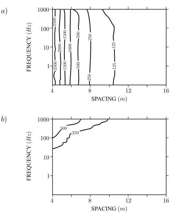
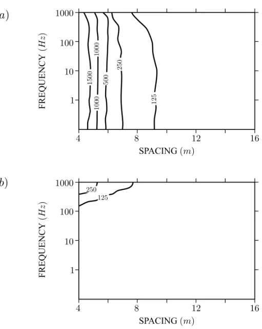
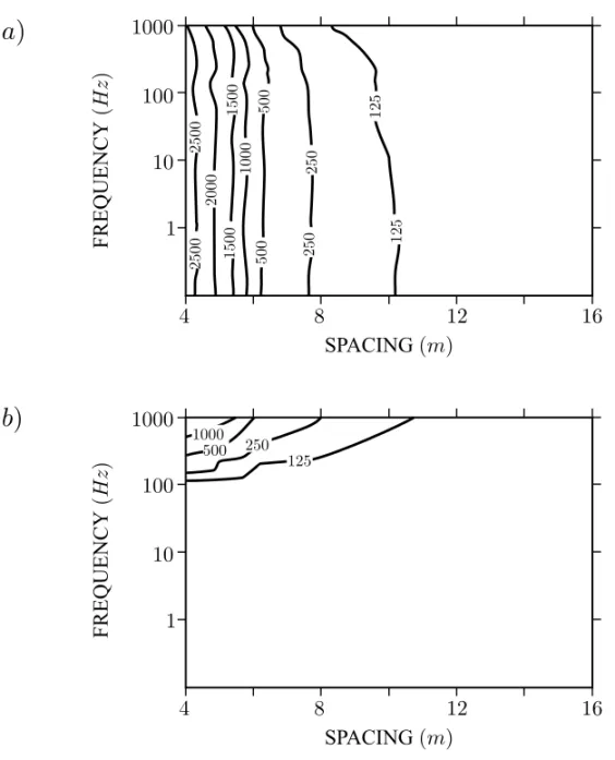
The experimental data provided the analysis of the real and imaginary parts of the electric field via pseudo-sections as a function of frequency and spac-ing. This enabled us to analyze the parameters of the induced polarization. These data are presented on Figures 2, 3, and 4, for the disk electrode with a radius of 0.075 m.

(4)

432 HERCULES DE SOUZA and EDSON E. S. SAMPAIO

Fig. 2 – Variation of (a) the real part and (b) the imaginary part of the electric field on the sea surface, in nV/m/mA as a function of frequency and lateral spacing (n=1,2,...,7).

Figures 2b, 3b and 4b show the imaginary part of the electric field. Its variation is mainly a function of frequency and not a function of spacing as it is for the real part. The imaginary part on the sea bottom is also higher than on the sea surface or in the middle of the water layer. This is also caused by the combination of the skin depth effect and the scattering at the sea surface.

PARAMETERS OF SPECTRAL INDUCED POLARIZATION

(5)

Fig. 3 – Variation of (a) the real part and (b) the imaginary part of the electric field at a depth of 7 m, in nV/m/mA, as a function of frequency and lateral spacing (n=1,2,...,7).

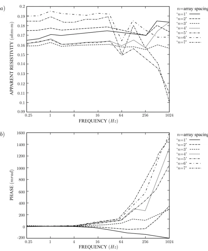
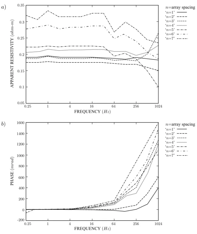
corrected for inductive coupling, on Figures 5, 6, and 7. Figures 5a, 6a and 7a show the behavior of the amplitude in_·m, and Figures 5b, 6b, and 7b show the behavior of the phase inmrad. In general the behavior in these figures is uniform below 64 Hz. Figure 5a shows the results for the electrodes placed on the sea surface. For array spacing 1 to 4 the curves show little fluctuations whereas for 5 to 7 and frequencies above 64 Hz, the plot shows a noisy behavior. Probably the noise is related to power lines close to the site of measurement. On this same figure we obtained a maximum variation

of 0.20_·mand a minimum variation of 0.16_·m for frequencieslowerthan 32 Hz.

(6)

Fig. 4 – Variation of (a) the real part and (b) the imaginary part of the electric field at the sea bottom, in nV/m/mA, as a function of frequency and lateral spacing (n=1,2,...,7).

frequency above 64 Hz. This is typical of elec-tromagnetic coupling (Ward 1990). The exception occurs only for the first array spacing of investiga-tion with the electrodes on the surface of the sea. For this case we should have the largest coupling effect on the phase value due to the vicinity be-tween the receiver electrodes and the transmitter electrodes. This anomalous behavior is caused prob-ably because of the interaction with the location of the equipment.

In Figures 5-7 we observe a large variation of

(7)

Fig. 5 – Behavior of (a) the amplitude and (b) the phase of the apparent resistivity on the sea surface, for the seven array spacing of investigation, and for the bar electrode (0.10 m).

(Hallof et al. 1979) state that the phase of the resistivity tends to show minimum values for a given frequency - the critical frequency. The value of this frequency is related to the grain size of the minerals

(8)

Fig. 6 – Behavior of (a) the amplitude and (b) the phase of the apparent resistivity 7 m deep, for the seven array spacing of investigation, and for the bar electrode (0.10 m).

PERCENT FREQUENCY EFFECT

We computed the Percent Frequency effect (PFE) employing the following expression:

P F E₌ ρ1.0−ρ8.0 ρ8.0 ×

100% (1)

(9)

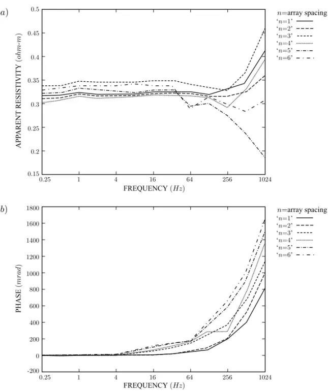
Fig. 7 – Behavior of (a) the amplitude and (b) the phase of the apparent resistivity at the sea bottom, for the six array spacing of investigation, and for the bar electrode (0.10 m).

the ‘‘ac’’ frequency value be low enough not to be severely affected by the EM coupling, which causes abnormal increase of the phase value and decrease of the mutual impedance value. (iii) That the ‘‘dc’’ frequency value be high enough not to be severely affected by the noise caused by flow, intermixing, and oscillation of the sea water at the Aratu Bay,

with a period of about 2 s. Probably this low fre-quency noise is the main cause for the maximum value of the apparent resistivity at 1.0 Hz, and the negative phase values below 1 Hz.

(10)

positive values of PFE at the sea surface, seven me-ter deep, and the sea bottom. Except for n ₌ 4 andn ₌5, where the PFE on the sea surface and 7 meter depth reaches 1.3%, 1.4% and 2.2%, the sea bottom yields the higher values of PFE, none of them above 2.5%. According to (Lima and Sharma 1992) the frequencies of 1 Hz and 8 Hz are within the range of frequencies where the diffusion mech-anism is the most important for polarization. Also previous drilling at the site yielded core samples of sediments containing disseminated clay. Therefore, this weak IP effect suggests the occurrence of mem-brane polarization due to the presence of clay in the sediments under the sea bottom.

FORWARD MODELING

We employed the algorithm developed by (Sato 2000) to compute forward models for the three sea levels of investigation. We used three layers for the initial model. The first layer has a resistivity of 0.19_·mand a thickness of 10.5 m, the second layer has a resistivity of 2.0_·mand a thickness of 6.0 m, and the third layer has a resistivity of 10.0_·m. The results of this modeling are shown on Figure 8 and indicate a good fitting between the experimental and the theoretical data. In order to minimize the ef-fect of frequency we employed the data of the lowest frequency, 0.25 Hz, to compare with the algorithm of (Sato 2000), which was developed for the direct-current case. The data represented in Figure 8 have been obtained with a different type of electrode and a different value of frequency from the data repre-sented in Table I, resulting in very different data for n=1.

The values of the theoretical curve for the sea surface approach the experimental values with a slight tendency to grow for the larger spacing. The theoretical curve at 7 m depth fits better the exper-imental data. We observed a point of crossing be-tween the theoretical curves for the sea surface and 7 m depth, both at an array spacing of 6 meters. The same crossing appears between the correspondent experimental curves at an array spacing of 7 m. The

theoretical curve of the sea bottom shows the same increase relative to the experimental data at a spac-ing of 6 m, a small decrease for 10 m and tends to grow for distances larger than 10 m.

The result obtained from this modeling empha-size the viability of the application of an electric method in the sea, because from the initial model it was possible to obtain a good fit between theoretical and the experimental curves.

EQUIVALENT ANALOG CIRCUIT

All rock samples are contaminated from the view-point of the physical chemist since the electrodes and electrolytes are anything but pure. Nevertheless, it is justifiable to employ equivalent circuits based on pure systems since a phenomenological explanation for rock behavior results (Ward 1990).

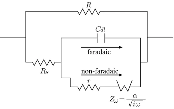
(Debye 1929) has formulated the phenomenon of polarization in rocks suitable for homogeneous substances. (Cole and Cole 1941) modified the ex-pression of Debye on empirical grounds to describe inclusive composite substances. However their ex-pression does not have a general validity. Subse-quent authors have suggested models and analytic expression for the complex electric conductivity in rock based on electric analog circuits to describe the induced polarization phenomenon. Among them we mention (Dias 1972, 2000) and (Pelton et al. 1978). Dias’ model, reproduced in Figure 9, is based on an analog fundamental circuit. It represents both the electrode and the membrane polarization phenom-ena, and it is based on the following equation: where

σ ₌σ0

1₊ βαλ

√

iω

1+βλ∗√_iω

, (2)

λ₌1+µ , (3)

λ∗₌1₊(1₋δ)µ , (4)

µ₌iωτ

1+√η

iω

, (5)

α₌m

1₋δ 1₋m

, (6)

β ₌ 1

(11)

TABLE I

Percent frequency effect (PFE) employing 1.0 Hz and 8.0 Hz and the vertical bar electrode (L = 0.03 m) for the given spreads n and positions.

n Sea surface Seven meters deep Sea bottom

ohm.m PFE% ohm.m PFE% ohm.m PFE%

1 0.142 0.0 0.206 1.0 0.300 1.7

0.142 0.204 0.295

2 0.164 0.6 0.187 1.1 0.318 1.0

0.163 0.185 0.315

3 0.153 0.7 0.199 1.0 0.332 1.2

0.152 0.197 0.328

4 0.157 1.3 0.224 1.4 0.314 0.6

0.155 0.221 0.312

5 0.159 0.6 0.230 2.2 0.328 1.2

0.158 0.235 0.324

6 0.190 1.1 0.290 0.0 0.330 1.9

0.188 0.290 0.324

In equations (2)-(7)ωis the angular frequency inrad/sand the main spectral parameters are de-scribed below

• σ0represents the conductivity of the DC cur-rent, in S/m.

• δis a non-dimensional parameter defined in the interval 0 ≤ δ < 1, which refers solely to the pore path representative of the locus where polarization is produced and involves only the components of the ohmic conduction.

• ηrepresents the relative strength between the ohmic component and the diffusion-produced component of the electrical current inside the electrical double layer. Its unit iss−1/2_{, and its} value ranges from 1 to about 150.

• τcorresponds to the relaxation time of the elec-trical double layer zone, due to the capacitance effect of the system. It is defined in the interval 10−7

≤τ _≥10−2_s.

• mis the ‘‘chargeability’’ (Seigel 1959), defined as a relation involving the asymptotic values of

the resistivity, in the interval 0_≤m <1.

(12)

Fig. 8 – Forward modeling of the apparent resistivity for the three sea levels of investigation. ZZAX and WATER represent respectively the theoretical and the experimental data at the sea surface. ZZBX and MIDDLE represent respectively the theoretical and the experimental data at seven meters deep. ZZCX and BOTTOM represent respectively the theoretical and the experimental data at the sea bottom. The experimental data are for f= 0.25 Hz, and the disk electrode with radius of 0.075 m.

observed and the theoretical data is less than 10%, though the observed conductivity is always larger than the theoretical.

Since each parameter has a physical mean-ing it is possible to define the dominant polariza-tion phenomenon by making its integrated analysis. Besides a relatively small PFE value, we observe from the data of Table II that: ‘‘m’’ is relativity large;τ is close to its minimum value; δ presents an average value; andηpresents a relatively large value. A small value ofτ indicates small grain size,

and a large value ofη indicates predominance of the diffusion mechanism. So the electric current flows mainly through the faradaic path, and the phe-nomenon is predominantly of a membrane polar-ization type. This is indicative of the presence of argillaceous sands, containing very few if any dis-seminated metallic minerals.

CONCLUSION

(13)

Fig. 9 – Reproduction of Dias’ model based on an analog fundamental circuit.

TABLE II

Dias’ parameters for the given electrode spreads n, employing the disk electrode(R= 0.025 m) at the sea bottom.

n m δ η τ % of fit

3 0.54 0.14 176.0 1.0_×10−7 _83.6 4 0.55 0.15 177.0 1.0×10−7 82.3 5 0.55 0.13 176.0 1.0×10−7 _82.5 6 0.54 0.14 177.0 1.0×10−7 _82.7

measurement of the vertical variation of the sea wa-ter electrical conductivity; and to define the geo-electric section of the sediments under the sea bot-tom. The vertical variation is obtained employing the smaller spread (n=1) and positioning the elec-trodes at different water depths. The geoelectric section is obtained by modeling the complete spread at different water depths. An optimum frequency spectrum between 1.0 Hz and 32.0 Hz, and a maxi-mum array spacing between the transmitter and the receiver dipoles,n <6, were defined. This choice of the measurement parameters restricted both the electromagnetic coupling and the noise caused by movements of the water in an environment with an

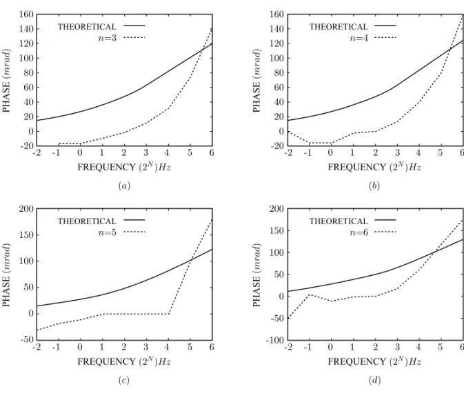
electrical conductivity of about 5.0 S/m. The fit ap-plying the L2 Norm to the phase of the apparent re-sistivity with an error of less than 18% is not good. But it served for the determination of Dias’ param-eters, which resulted in a good fit between the theo-retical and the experimental curves of the modulus of the apparent conductivity.

The modulus of the apparent resistivity repre-sents an adequate parameter for geoelectric tation under the sea. On the other hand the interpre-tation of spectral induced polarization phenomena employing both the modulus and the phase data de-fined the type of phenomenon and the source of a low magnitude IP effect in the sediments under the sea bottom. We presented the behavior of only one type of electrode per analysis, because of the relative repeatability of the measurements.

ACKNOWLEDGMENTS

(14)

Fig. 10 – Fit between the theoretical and experimental phase data, obtained by inversion of Dias’ parameters employing L2 Norm, at the sea bottom: n = array spacing (a) n=3; (b) n=4; (c) n=5; (d) n=6.

RESUMO

Relativamente poucas investigações têm empregado

mé-todos elétricos no ambiente submarino, o qual pode ser

promissor para depósitos minerais ou ameaçado por

pro-blemas ambientais. Nós medimos o campo elétrico

usan-do eletrousan-dos em forma de disco e de barra na água usan-do

mar, em três níveis distintos: superfície, sete metros de

profundidade, e fundo do mar a dez metros de

profundi-dade, empregando um dispositivo dipolo-dipolo com 2m

de afastamento, 7 níveis de investigação e 13 valores de

freqüência a intervalos de (2Nhertz, N = –2, –1, 0, 1, 2,

... 10). A medida permitiu a análise do campo elétrico

como uma função de freqüência e afastamento, e da

po-larização induzida espectral. A modelagem e a

interpre-tação da resistividade aparente se ajustaram bem aos dados

de perfurações prévias. A análise do espectro da função

complexa da resistividade aparente e sua comparação com

circuitos equivalentes geraram informações a respeito de

tamanho do grão, composição mineral e do aspecto

prin-cipal do fenômeno de polarização ocorrendo abaixo do

fundo do mar. Portanto, o resultado da presente pesquisa

mostra ser exeqüível medir a variação da resistividade da

água do mar, assim como a resistividade dos sedimentos

do fundo do mar in situ.

Palavras-chave: resistividade aparente complexa,

(15)

Fig. 11 – Comparison between the experimental and theoretical apparent conductivity (S/m) with disk electrode (R= 0.025m) at the sea bottom, for array spacing n=3.

REFERENCES

Baumgartner F.1996. A new method for geoelectrical investigations underwater. Geoph Prosp 44: 71-98.

Chave AD and Cox CS.1982. Controlled electromag-netic sources for measuring electrical conductivity beneath the oceans, 1. Forward problem and model study. J Geoph Res 87: 5327-5338.

Chave AD, Constable SC and Edwards RN.1991. Electrical exploration methods for the seafloor. In:

Nabighian MN(Ed.); Electromagnetic methods in applied geophysics, vol II, Applications, Parts A and B. Tulsa: SEG, p. 931-962.

Cheesman SJ, Edwards RN and Chave AD.1987. On the theory of seafloor conductivity mapping using transient electromagnetic systems. Geophysics 52: 204-217.

Cheesman SJ, Edwards RN and Law LK.1990. A test of a short-baseline sea floor transient electromagnetic system. Geophys J Int 103: 431-437.

Cheesman SJ, Law LK and Edwards RN.1991. Poros-ity determinations of sediments in knight inlet using a transient electromagnetic system. Geo-marine Let-ters 11: 84-89.

Cole KS and Cole RH.1941. Dispersion and absorp-tion in dielectrics. J Chem Phys 9: 341-351.

Debye P.1929. Polar molecules. The Chemical Catalog Co Inc Also (1945) Dover Publications.

Dias CA. 1972. Analytical model for a polarizable medium at radio and lower frequencies. J Geophys Res 77: 4945-4956.

Dias CA.2000. Developments in a model to describe low-frequency electrical polarization of rocks. Geo-physics 65: 437-451.

Edwards RN and Chave AD.1986. A transient electric dipole-dipole method for mapping the conductivity of the sea floor. Geophysics 51: 984-987.

(16)

crust by a modified magnetometric resistivity method. J Geophys Res 86: 11609-11615.

Hallof PG, Cartwright PA and Pelton WH.1979. The use of the Phoenix IPV-2 phase IP receiver for discrimination between sulfides and graphite. In:

49th Annual International Meeting, New Or-leans. Expanded Abstract, SEG.

Lima OL and Sharma MM.1992. A generalized Max-well-Wagner theory for membrane polarization in shale sands. Geophysics 57: 431-440.

Nabighian MN and Elliot CL. 1976. Nega-tive induced-polarization effects from layered media. Geophysics 41: 1236-1255.

Pelton WH, Ward SH, Hallof PG, Sill WR and Nelson PH.1978. Mineral discrimination and removal of inductive coupling with multi-frequency IP. Geophysics 43: 588-609.

Petiau G and Dupis A.1980. Noise, temperature coeffi-cient, and long time stability of electrodes for telluric observations. Geoph Prosp 28:792-804.

Porsani MJ, Stoffa PL, Sen M and Chunduru RK.

2000. Fitness functions, genetic algorithms and hy-brid optimization in seismic waveform inversion. J. Seismic Exploration 9: 143-164.

Sampaio ES, Santos AB and Sato HK.1998. Spec-tral induced polarization and mineral discrimination. In: 68th Annual International Meeting, New Orleans. Expanded Abstracts, SEG.

Sato HK.2000. Potential field from a dc current source arbitrarily located in a nonuniform layered medium. Geophysics 65: 1726-1732.

Seigel HO.1959. Mathematical formulation and type curves for induced polarization. Geophysics 24: 547-565.

Ward SH.1990. Resistivity and induced polarization methods. In:Ward SH(Ed.); Geotechnical and En-vironmental Geophysics. Tulsa, SEG.