Optimization of toolpath trajectories on arbitrary surfaces
by MIGUELBELBUTGASPAR ANDNELSONMARTINS-FERREIRA
Centre for Rapid and Sustainable Product Development, Polytechnic Institute of Leiria, Marinha Grande, Portugal
Abstract: Given an arbitrary region on the plane, modelled as a graph with a symmetry, we describe a procedure to find the best orientation for slicing, via a zigzag tool-path trajectory based curve, in order to minimize its disconti-nuities. We also develop some directions on how to generalize the procedure up to the level of optimizing tool-path trajectories on arbitrary surfaces rather than planar regions only.
Keywords: toolpath generation zig-zag strategy optimization additive manufacturing.
1
Introduction
The generation of optimized tool-path trajectories is a de-manding and computationally difficult problem that has been considered since the early ages of CAD/CAM sys-tems of rapid prototyping and rapid manufacturing of new products in the area of industry and enterprises in general. Hence it has already been addressed for the last thirty years or so. Nevertheless, the more recent applica-tion of 3-D printing, namely to medical applicaapplica-tion has provided new and challenging problems in this area. The old methods that were already well established are no longer applicable as the technology has moved from the point of view of subtractive manufacturing to additive manufacturing, suggesting new perspectives and strate-gies of machine toolpath generation. One of the big con-straints of this systems is the necessity of a good finishing detail level. In particular it is a heavy handicap the im-possibility of always having a continuous toolpath for a whole region at a given layer. We will present some as-pect of implementation and optimization for this kind of toolpath generation systems. We will give special atten-tion to the so-called zig-zag strategy, giving some details on how it is modelled and implemented in a computer system, and also on how to optimize the number of dis-continuities in the path. These results are already imple-mented for planar regions but we will also give further indications on how they can be extended to the level of trajectories to cover regions in arbitrary triangulated sur-faces. In this text we will also explain how to develop a procedure to automatically generate toolpath trajectories in abstract triangular spaces, with possibly applications to other areas of interest rather that the rapid-prototyping and rapid-manufacturing of products for the industry.
This text is only an extended abstract of a ongoing work. It presents ideas and algorithms that can be im-plemented in any computational system such as Matlab. It considers the case of tool-path optimization trajecto-ries in arbitrary planar regions defined by a graph with a
symmetry, as it is defined in [1]. The trajectories by them-selves are generated with an algorithm described in [2]. At the end we give some directions on how to generalize the results for arbitrary surfaces.
2
Establishing the framework
As it is explained in [1], an arbitrary region in the plane may be described as a graph with a symmetry, that is a system(A, B, d, c, ϕ) in which
A d /
/
c
/
/B
is a directed graph and
ϕ: A → A
is a bijection such that dϕ = c. As usual, the elements in A are considered as directed edges with an element a∈ A pictured as
d(a) a //c(a) ,
and its image by ϕ considered as the successor directed edge defining the contour of the region
d(a) a / /c(a)
ϕ(a)
/
/cϕ(a) ,
with the assumption that its interior is always on the left. For practical purposes we give a specific example which will be used throughout the text to illustrate the several steps involved in the outlined procedure.
3 FINDING THE BEST ORIENTATION FOR SLICING
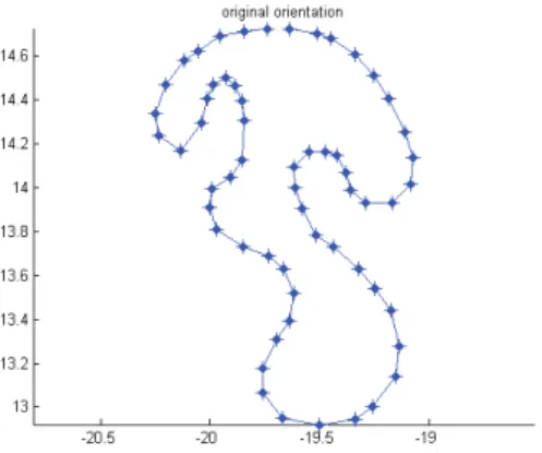
Fig. 1 - Original curve orientation.
The example is depicted in Figure 1 above and it is defined by the following data, presented as a sequence of directed edges, each one determined by its endpoints, encoded in a vector named P . In other words, we have a set A= {1, 2, 3, . . . , 58, 59}, and a set B ⊂ R2. The vector
P is displayed as: P = −19.3566 , 13.9876 −19.2874 , 13.9291 −19.1665 , 13.9291 −19.0801 , 14.0168 −19.0719 , 14.1372 −19.1089 , 14.2534 −19.1829 , 14.4065 −19.2515 , 14.5121 −19.3360 , 14.6071 −19.4487 , 14.6820 −19.5121 , 14.7039 −19.6388 , 14.7259 −19.7368 , 14.7259 −19.8404 , 14.7113 −19.9556 , 14.6893 −20.0536 , 14.6235 −20.1169 , 14.5797 −20.2033 , 14.4700 −20.2494 , 14.3385 −20.2321 , 14.2361 −20.1342 , 14.1703 −20.0363 , 14.2946 −20.0132 , 14.4042 −19.9853 , 14.4698 −19.9246 , 14.5015 −19.8824 , 14.4645 −19.8507 , 14.3959 −19.8402 , 14.3062 −19.8507 , 14.1267 . . . . . . −19.9035 , 14.0475 −19.9880 , 13.9947 −19.9985 , 13.9102 −19.9672 , 13.8121 −19.8462 , 13.7317 −19.7310 , 13.6879 −19.6619 , 13.6294 −19.6158 , 13.5197 −19.6388 , 13.3955 −19.6964 , 13.3077 −19.7598 , 13.1762 −19.7598 , 13.0665 −19.6676 , 12.9496 −19.5006 , 12.9203 −19.3335 , 12.9423 −19.2586 , 13.0007 −19.1492 , 13.1396 −19.1377 , 13.2785 −19.1722 , 13.4393 −19.2471 , 13.5417 −19.3220 , 13.6294 −19.4372 , 13.7317 −19.5179 , 13.7829 −19.5812 , 13.9072 −19.6100 , 14.0022 −19.6158 , 14.0972 −19.5467 , 14.1630 −19.4718 , 14.1630 −19.4199 , 14.1484 −19.3796 , 14.0680
The maps d, c are, respectively, the first and second components, while the map ϕ is defined by ϕ(i) = i + 1 if i≤ 59 and ϕ(59) = 1. The maps d and c may be also seen in terms of the vector P as d(i) = P (i, 1), c(i) = P (i, 2).
In the next section we assume a vector such as P is de-fined and will deduce a collection of possible orientations which minimize the tool-path trajectories, as exemplified in Figure 2.
Fig. 2 - Zig-zag toolpath trajectories.
3
Finding the best orientation for
slicing
Given P as before, we want to minimize the number of inflection points for a scan angle θ. The algorithm is de-scribed in pseudo-code, using Matlab syntax.
1 I n p u t : P − n−by −2, polygon ’ s v e r t i c e s as 2 rows ( x , y )
3 Output : Aopt − m−by −2, m ranges ( amin , amax) 4 o f o p t i m a l a n g l e s . 6 % c o n v e r t t o c o m p l e x form 7 Pc=P ∗ [ 1 ; i ] ; 9 % O b t a i n t h e o r i e n t a t i o n o f e a c h e d g e : 10 A=angle ( Pc ( [ 2 : end , 1 ] )−Pc ) ∗180/ pi 12 % Get i n n e r a n g l e s 13 IA=mod(mod(180−A,360)+mod(A ( [ 2 : end , 1 ] ) ,360) ,360) ;
We are interested in the concavities, i.e, !"#$%. At a convex vertex, as the scan slope passes the emerging edge’s slope, that vertex ceases to be an inflection point. At the same time, the next vertex becomes a new inflec-tion point, if it is convex, too. So as this scanning slope is reached, no new net inflection points are added. Some-thing different occurs when we consider concave vertices: as we reach the emerging edge’s slope, a new inflection point appears (in fact, two).
When two successive vertices are concave, no net in-flection point is added, either.
1 % Concave v e r t i c e s : 2 CC=IA >180 4 % Changes , t h a t i s , s e q u e n c e s c o n v e x−>c o n c a v e 5 % T h i s i s t h e non−t r i v i a l d i f f i c u l t p a r t 6 DC=d i f f (CC ( [ end , 1 : end ] ) ) 8 % S o r t t h e a n g l e s (mod 180) : 9 A3=s o r t r o w s ( [mod(A, 1 8 0 ) , DC] )
By cummulative sum of the net change in number of inflection points, we find the range of theta with the min-imum amount of infl. points:
4 CONCLUSION
1 A4=[A3 ( : , 1 ) , cumsum(A3 ( : , 2 ) ) ] 3 % E x t r a c t t h e n e e d e d i n f o r m a t i o n :
4 ixm=f i n d (A4 ( : , 2 )==min(A4 ( : , 2 ) ) ) ; 6 tmp=[ixm−ixm ( [ end , 1 : end−1]) , . . . 7 ixm ( [ 2 : end , 1 ] )−ixm]~=1 8 ixm=[ixm ( tmp ( : , 1 ) ) , ixm ( tmp ( : , 2 ) ) ] 9 AOpt=[A4( ixm ( : , 1 ) , 1 ) , A4( ixm ( : , 2 ) , 1 ) ]
The result of each of the preceding steps applied to the input data P as defined in the previous section is pre-sented at the end.
The output result is presented as ranges of angles in the form
!"#$%!&' !"#$ (&) !"#$%!*' !"#$ (*) +++
!"#$%!,' !"#$ (,
which for the working example has the following result.
-./0 1
2 *3+445*
&45+&46& &32+&6*7
This means that for rotations with an angle between 0 and 27.5592 degrees, there are a minimum number of discontinuities in the tool-path trajectory. For rotation an-gles ranging from27.5592 to 159.1581 degrees, the num-ber of discontinuities is increasing while it again attends a minimum when the rotation angle is between159.1581 and170.1824. Again form 170.1824 to 360 there is a larger number of discontinuities.
The suggested optimal angles are displayed in the fol-lowing pictures.
4
Conclusion
To conclude we remark that the procedure may be gen-eralized to the context where the region is not necessar-ily planar but is embedded into an arbitrary surface in the space. This is important for the purpose of generating tool-path trajectories for rapid manufacturing and rapid prototyping since it will allow a greater number of ap-plications. To to that we will only need to transform the structure used in [2] by imposing that the linking lines between two intersected points in the same g-component, to use the nomenclature of [2], are no longer straight lines but are geodesic path instead. This part is not yet implemented. It will use algorithms for working with
REFERENCES
geodesic paths and then combine the structure(E, r, g, s) used in [2],requiring also the geometric information con-cerning the convexity of each edge, used in here, obtain-ing thus the same results for surfaces.
References
[1] Gaspar, Miguel Belbut, and Nelson Martins-Ferreira.
A procedure for computing the symmetric difference of
regions defined by polygonal curves, Journal of
Sym-bolic Computation 61 (2014) 53–65.
[2] Miguel Belbut Gaspar, Nelson Martins-Ferreira, Sobre
estratégias de varrimento contínuo para o preenchi-mento de regiões arbitrárias no plano, Boletim da
So-ciedade Portuguesa de Matemática (2010), no. Espe-cial, 78–86.
Appendix
Below is presented the output of each relevant step in the execution of the procedure described in the text. Each vector is listed from top to bottom and from left to right and from one page to the next one.
! "#$%&'()# "#*+&((*' "(+&#$,) "+$&$,+' "%%&'#$+ "$)&-*#( "*)&$%#* "'+&$)*# "#))&,)*% "#$%&$($$ "##,&+#%( "()&)))) ",#&+'#$ "(&($-$ +&*+--%+&(-+$ ,#&+'#$ -,&$,-$ #)$&#$($ #$'&#(*# #%)&*-'( #%-&%-,$ #*+&')*- ##+&)#'-#)'&-'#$ (%&*'--*%&,-*) ) "#,&+*-, "'%&%'+-"+*&)#)$ "*)&$%#* ) *,&*%$% -'&#),) #)+&+),% ##,&+'(% #$%&)$%( #%#&'%%, #*'&%(-+ #')&()(' #+)&#-$* #-)&)))) "#+#&(+*$ "#'(&$$$' "#*'&#),+ "#*,&%)(' "#$-&$%-- "#)(&%)#-"-)&*#,* "%%&-(*% ,#&+'#$ +-&#%$' ''&(*$) $+&,,($ "*#&#-,( "',&$$*( "-%&$()$ "(%&%'', .. ! ) # # # # ) ) ) ) # # # # # # # # # # # # # ) ) ) ) ) ) ) ) # # # # # # # # # # # # # # # # # # # # # # ) ) ) ) ) ) ) /. ! ) # ) ) ) "# ) ) ) # ) ) ) ) ) ) ) ) ) ) ) ) "# ) ) ) ) ) ) ) # ) ) ) ) ) ) ) ) ) ) ) ) ) ) ) ) ) ) ) ) ) "# ) ) ) ) ) )
REFERENCES ! " # # # # # # $%&$'' # '%#()' # *#%$$$& # ($%))+( # !(%##)& *%#### !!%'+&! # !&%,+#& # !$%+'$( # &!%)'&# # &)%&!(! # )*%$,*( # )*%$,*( # )*%$,*( # ),%!#++ # ),%$#$' *%#### ,&%(',* # ,,%+&(# # $#%,+'( # $'%*!(, -*%#### $+%&+)$ # '(%'$)# # ')%()'( # ',%*#)# # ',%,!!) # +#%#### # +!%&,'' # +,%$#+' # ++%)'&, # *#(%*(+( # *#)%+'+' *%#### *#,%',*( # *#$%$#)! # *#$%$&(& # **(%$+)+ # **&%$$)* # **)%$,+! # **,%,!(( # **$%#*,' # *(!%#(!+ # *(,%*+&* # *('%(!'' # *!#%&',+ # *!*%,!!) # *!'%!')( # *!'%'*&* # *!+%$,', # *!+%$,', # *&,%*#)$ # *&,%!'$! # *&,%!+'$ # *&$%,#&' -*%#### *)+%*)'* -*%#### *,#%+#+, # *,&%()*) # *$#%#$*' # *$#%*'(& # & " # # # # # # $%&$'' # '%#()' # *#%$$$& # ($%))+( # !(%##)& *%#### !!%'+&! *%#### !&%,+#& *%#### !$%+'$( *%#### &!%)'&# *%#### &)%&!(! *%#### )*%$,*( *%#### )*%$,*( *%#### )*%$,*( *%#### ),%!#++ *%#### ),%$#$' (%#### ,&%(',* (%#### ,,%+&(# (%#### $#%,+'( (%#### $'%*!(, *%#### $+%&+)$ *%#### '(%'$)# *%#### ')%()'( *%#### ',%*#)# *%#### ',%,!!) *%#### +#%#### *%#### +!%&,'' *%#### +,%$#+' *%#### ++%)'&, *%#### *#(%*(+( *%#### *#)%+'+' (%#### *#,%',*( (%#### *#$%$#)! (%#### *#$%$&(& (%#### **(%$+)+ (%#### **&%$$)* (%#### **)%$,+! (%#### **,%,!(( (%#### **$%#*,' (%#### *(!%#(!+ (%#### *(,%*+&* (%#### *('%(!'' (%#### *!#%&',+ (%#### *!*%,!!) (%#### *!'%!')( (%#### *!'%'*&* (%#### *!+%$,', (%#### *!+%$,', (%#### *&,%*#)$ (%#### *&,%!'$! (%#### *&,%!+'$ (%#### *&$%,#&' *%#### *)+%*)'* # *,#%+#+, # *,&%()*) # *$#%#$*' # *$#%*'(& # ./0 " * # # # # # # # # # # # # * * # # # # # # # # * 12/ " * $ )) )+