On the growth effects of barriers to trade

❊♥s❛✐♦s ❊❝♦♥ô♠✐❝♦s

❊s❝♦❧❛ ❞❡

Pós✲●r❛❞✉❛çã♦

❡♠ ❊❝♦♥♦♠✐❛

❞❛ ❋✉♥❞❛çã♦

●❡t✉❧✐♦ ❱❛r❣❛s

◆◦ ✸✺✸ ■❙❙◆ ✵✶✵✹✲✽✾✶✵

❖♥ t❤❡ ●r♦✇t❤ ❊✛❡❝ts ♦❢ ❇❛rr✐❡rs t♦ ❚r❛❞❡

❆❧❜❡rt♦ ❚r❡❥♦s✱ P❡❞r♦ ❈❛✈❛❧❝❛♥t✐ ●♦♠❡s ❋❡rr❡✐r❛

❖s ❛rt✐❣♦s ♣✉❜❧✐❝❛❞♦s sã♦ ❞❡ ✐♥t❡✐r❛ r❡s♣♦♥s❛❜✐❧✐❞❛❞❡ ❞❡ s❡✉s ❛✉t♦r❡s✳ ❆s

♦♣✐♥✐õ❡s ♥❡❧❡s ❡♠✐t✐❞❛s ♥ã♦ ❡①♣r✐♠❡♠✱ ♥❡❝❡ss❛r✐❛♠❡♥t❡✱ ♦ ♣♦♥t♦ ❞❡ ✈✐st❛ ❞❛

❋✉♥❞❛çã♦ ●❡t✉❧✐♦ ❱❛r❣❛s✳

❊❙❈❖▲❆ ❉❊ PÓ❙✲●❘❆❉❯❆➬➹❖ ❊▼ ❊❈❖◆❖▼■❆ ❉✐r❡t♦r ●❡r❛❧✿ ❘❡♥❛t♦ ❋r❛❣❡❧❧✐ ❈❛r❞♦s♦

❉✐r❡t♦r ❞❡ ❊♥s✐♥♦✿ ▲✉✐s ❍❡♥r✐q✉❡ ❇❡rt♦❧✐♥♦ ❇r❛✐❞♦ ❉✐r❡t♦r ❞❡ P❡sq✉✐s❛✿ ❏♦ã♦ ❱✐❝t♦r ■ss❧❡r

❉✐r❡t♦r ❞❡ P✉❜❧✐❝❛çõ❡s ❈✐❡♥tí✜❝❛s✿ ❘✐❝❛r❞♦ ❞❡ ❖❧✐✈❡✐r❛ ❈❛✈❛❧❝❛♥t✐

❚r❡❥♦s✱ ❆❧❜❡rt♦

❖♥ t❤❡ ●r♦✇t❤ ❊❢❢❡❝ts ♦❢ ❇❛rr✐❡rs t♦ ❚r❛❞❡✴

❆❧❜❡rt♦ ❚r❡❥♦s✱ P❡❞r♦ ❈❛✈❛❧❝❛♥t✐ ●♦♠❡s ❋❡rr❡✐r❛ ✕ ❘✐♦ ❞❡ ❏❛♥❡✐r♦ ✿ ❋●❱✱❊P●❊✱ ✷✵✶✵

✭❊♥s❛✐♦s ❊❝♦♥ô♠✐❝♦s❀ ✸✺✸✮

■♥❝❧✉✐ ❜✐❜❧✐♦❣r❛❢✐❛✳

On the Growth E¤ects of Barriers to Trade

¤

Pedro Cavalcanti Ferreira

EPGE - Fundação Getulio Vargas

Alberto Trejos

Northwestern University

& INCAE

A bst r act

We study the macroeconomic e¤ects of international trade policy by integrating a Hecksher-Ohlin trade model into an optimal growth framework. The model predicts that an open economy will have higher factor productivity and faster growth. Also, under protectionist poli-cies there may be “ development traps,” or additional steady states with low income. In the last case, higher tari¤s imply lower incomes, so that the large cross-country di¤erences in barriers to trade may ex-plain part of the huge dispersion of per capita income observed across countries. The model simulation shows that the link between trade and macroeconomic performance may be quantitatively important.

1 I nt r oduct ion

There is a large disparity across countries in income, growth rates, and other key macroeconomic variables. Abundant empirical research has studied whether those cross-country variations are related to di¤erences in interna-tional trade policy, …nding that open economies have higher levels of capital

¤_{We are grateful to multiple audiences for their input. The …rst author acknowledges}

wit h gratitude the …nancial support of CNPq and PRONEX; the second author of the National Science Foundation.

y_{Email: ferreira@fgv.br}

and total factor productivity, achieve faster growth, and enjoy better chances of convergence in per-capita output. This paper addresses whether the sim-plest comparative advantage arguments, when framed in a macroeconomic model, can explain the link between trade policy and macroeconomic per-formance, and account for a relevant portion of the observed income gap between rich and poor nations.

Evidence regarding the link between trade liberalization and output lev-els is provided by Frankel and Romer (1996) and by Hall and Jones (1999). They elaborate that openness (namely, low tari¤s and low incidence of quo-tas and other non-tari¤ trade barriers) increases income per-capita both by enhancing capital accumulation and, notably, by expanding productivity. Evidence regarding the positive relationship between open trade policy and growth rates, which is discussed in Krueger (1997), has been documented recently by Edwards (1997), Frankel, Romer and Cyrus (1996), Harrison (1995), Lee (1996) and Taylor (1996), using various types of data samples and techniques. Previous empirical work on the same topic is also surveyed in Edwards (1993). Finally, evidence regarding the relationship between trade policy and convergence is provided in Sachs and Warner (1995), who show that among the countries that they consider open to trade, one cannot statis-tically reject convergence, while the same is not true in a broader sample of countries. To us, this …nding suggests that very poor countries that choose isolationist trade policies set for themselves “ development traps” , and that the pervasiveness of protectionism among LDC´ s may be responsible for the “ twin-peak distribution” suggested by Quah (1996).

These empirical results have been derived from data panels that include a majority of poor countries. For those nations, di¤erences in factor endow-ments with respect to their wealthier main trading partners are a strong a motive for trade, probably as important as any other. Then, without detri-ment to other possible channels for the macroeconomic e¤ects of trade policy, it seems natural to inquire whether the links mentioned above between trade liberalization and macroeconomic performace can be accounted for in a com-parative advantage framework in thevein of the Hecksher-Ohlin model.1 _Yet,

1_{Most previous e¤orts to explain the link between trade and growth emphasize other}

this is not a channel that many believe would be fruitful. As Stiglitz (1998) points out, we understand well why exploiting comparative advantage gener-ates static welfare gains, yet the dynamic improvement in aggregate output that the data suggests is still largely unexplained.2

We merge a factor-endowment trade structure into the standard neoclas-sical growth model. Like in Corden (1971), Trejos (1992) or Ventura (1997) in order to do this we assume two tradable and non-storable intermediate goods, used in the production of a non-tradable …nal good. This has the ad-vantage that the potentially complex dynamic trade problem can be solved sequentially. First one solves the static trade and factor allocation prob-lem; the solution takes the form of an endogenous mapping between factor endowments and aggregate output. Second, one solves the optimal growth problem, treating that mapping as an exogenously given production func-tion. We focus on a small, price-taking economy, which trades with a larger “ world economy” . We interpret the latter to be a developed country (or group of countries) that has already converged to a balanced growth path and for which, due to its size, trade is relatively unimportant.

The equilibrium mapping that shows the relationship between factors and output, and plays the role of the small economy´ s implicit production function, is a¤ected by tari¤s and by international prices. Speci…cally, an increase in trade barriers, or a worsening in terms of trade, have an e¤ect quite similar to a decrease in productivity. In that sense, the model can be useful in understanding the relationship between openness and measured TFP. Furthermore, it is the case that this mapping, under no trade, takes the form of a standard, constant returns to scale Cobb-Douglas function, while for the small, trading economy the mapping is qualitatively di¤erent, and not even necessarily concave. As a consequence, we …nd that a trading economy may have development traps, in the sense that there are not one but two locally asymptotically stable balanced growth paths. 3 _{The higher}

2_{Speci…cally, he writ es ´ ´ Interestingly, the process by which trade liberalization leads to}

enhanced productivity is not fully understood. The standard Hecksher-Ohlin theory predicts that countries will shift intersectorally, moving along their production possibility frontier, producing more of what they are better at and trading for what they are worse at. In reality, the main gains from trade seem to come intertemporally, from an outward shift in the production possibility frontier as a result of increased e¢ ciency, with little sectoral shift. Understanding the causes of this improvement in e¢ ciency requires an understanding of the links between trade, competition, and liberalization. This is an area that needs to be pursued further.”

balanced growth path is largely invariant to tari¤s, while the lower one is sensitive to trade policy so that, the higher the barriers to trade, the lower the levels of inputs, productivity and output.4

We calibratethemodel to see what is the order of magnitude of the e¤ects that it predicts for trade policy. The calibration is conservative, in the sense that the factor shares are not allowed to di¤er much across tradeable goods, thus limiting the size of the potential gains from trade. In fact, under the chosen parameters the static e¤ects from trade are essentially negligible for the world´ s rich countries. Still, even under those parameters gains from trade can be important for countries that are relatively poor. For instance, for a country with one-…fth of US output the static di¤erence between having 10% tari¤s and 100% tari¤s can be 7.5% of total factor productivity. One can also calculate the sensitivity of the output level of the development trap (the lower steady state), as one changes the tari¤ rate. The e¤ects are, again, large. For our baseline parameters, at very low tari¤s the trap´ s output per capita is nine-tenths of the output of the world´ s richest economy. Meanwhile, at 40% tari¤s, the economy in a trap has only one-third of the richest country´ s income; at 100% tari¤s, one-…fth. In summary, a closed economy will be less productive in the short run, grow more slowly towards steady state, and perhaps even converge to a lower steady state level of output, than an open economy.

Section 2 presents the model, and Section 3 derives thetheoretical results. The calibration and quanti…cation of the results is performed in Section 4. Section 5 concludes.

of convergence to them. Trejos (1992) compares the transit ional dynamics under free trade to those under no trade. The main result is t hat a very poor economy initially grows faster under free trade than in autarky.

4_{Following Parente and Prescott (1994), researchers have att empted to explain the}

2 T he economy

Time is discrete and unbounded. Our representative country is populated by a continuum of identical, in…nitely-lived individuals. There are three goods produced in this economy. Two of those goods, called A and B, are non-storable intermediate products. They are only used to make the other good, called Y, a …nal product that can be consumed or invested. There are also two factors of production in this economy: labor L and physical capital K. The endowment of labor, measured in e¢ ciency units, grows at an exogenous rate¹, due to both demographic expansion and technical progress.

The technology is as follows: physical capital and labor can be used in the production of the intermediate goods A and B, with constant returns Cobb-Douglas technologies:

A = K®a

A L1¡ ®A a

B = K®b

B L1¡ ®B b:

Without loss of generality, we assume that A is the labor-intensive good, so ®a < ®b. The production of the …nal goodY uses the intermediate goods:5

Y = £ a°_b1¡ °_{: (1)}

Final goods can be used in either consumption or investment. The law of motion for capital is

K0_{= (1¡ ±)K + Y ¡ C (2)}

The representative consumer owns the capital, and faces the standard in-tertemporal maximization problem, with instantaneous log utility and dis-count rate denoted ¯. All markets are perfectly competitive. The ordinary market clearing conditions for both factors are

K ¸ Ka+ Kb

L ¸ La+ Lb

The economy is only one of many others in the world, and is small, at least compared to a certain very large country, which we just call the world

5_{The results are not changed signi…cantly if we assume that factors are used also in the}

economy. The relative sizes of the two economies mean that, if they trade, the small economy will be a price-taker, as the prices at which they trade are the same as the world-economy´ s autarkic prices.6 _{We assume that}

physi-cal and legal characteristics imply that only the intermediate goodsA and B can be exchanged internationally; our small economy´ s government im-poses a ‡at, ad-valorem tari¤¿;and the proceeds from tari¤s are transferred back to households. Factors, …nal output or any form of …nancial obligation cannot be traded. This also implies that there will always be trade balance in intermediate goods. All markets that do exist are assumed to be per-fectly competitive. In the baseline scenario, all parameters, preferences and technologies are assumed to be common across the two countries.

Since it can be shown that under no trade this model has a unique, globally stable balanced growth path with growth rate¹ (a steady state if we measure capital and output in per-labor units) we can assume that the world economy has already converged to said steady state, with a capital-labor ratio denoted k¤_{. That means that the international relative price of} A in terms of B, denoted p, is constant, as it is the no-trade equilibrium price in the world economy, pinned down by k¤_{. In our small economy, the}

domestic relative price of A in terms of B (which may di¤er from pdue to tari¤s) is denotedq. The domestic price of …nal output Y (again in terms of B) is denoted ¼.

3 Equilibr ium

The procedure used to …nd equilibria for the model is the following. First, we solve for the allocation of capital K and labor L among the production of A andB, the quantitiesaandbof intermediate goods used domestically, and the amount of …nal output Y that is produced. This is a static problem, which yields an equilibrium mapping

Y = F (K ; Lj¿; p)

that relates …nal output with factor endowments. Second, we use that equi-librium mapping F as if it was an exogenously given technology, and solve the standard dynamic problem that emerges as a result.

6_{This because trade with t he small economy is a miniscule fraction of economic activity}

To get F notice that the equilibrium solutions for fA; B ; a; b; Ki; Lig must

satisfy, each period, the following properties7

1. The allocation of K and L maximizes the value of intermediate-good output at domestic prices, given endowments and technology:

A; B = argmax

A ;B qA + B s:t: A · K®a

A L1¡ ®A a

B · K®a

B L1¡ ®B b

K ¸ KA + KB

L ¸ LA + LB

2. Producers of …nal goods maximize pro…ts, taking domestic prices as given

a; b = argmax

a;b ¼a

°_b1¡ ° _{¡ qa¡ b}

3. With no factor ‡ows and no debt there is current account balance

pa + b = pA + B

4. The local prices must satisfy an after-tari¤ law of one price

q = (

p=(1 + ¿) i f K =L < k¤

p¢(1 + ¿) if K =L > k¤ :

Based on the requisites 1-4 mentioned above, one can derive the equilib-rium relationship F. The basic calculations are relegated to the Appendix, while here we stress what is important, as follows

1. If the capital-labor ratio k = K =L is very di¤erent from the world´ s k¤_{, the economy will specialize in the production of only one}

interme-diate good: the one that uses intensively the factor that is relatively abundant locally. Thus, there are critical levelskbA < k¤ and bkB > k¤

such that if k · kbA then the country only producesA, and if k ¸ kbB

then the country only producesB :In those cases,Y is a Cobb-Douglas

7_{For an exposition on the basic Hecksher-Ohlin factor endowments model, see Dixit}

function of K and L, with capital share®a or ®b, depending on which

intermediate good gets produced. Furthermore, the critical valuesbkA

and kbB are sensitive to ¿. In particular, with higher tari¤s the

econ-omy is less prone to specialize, so @bkA=@¿ < 0 and @bkB=@¿ > 0, with

b

kA ! 0and kbB ! 1 as¿! 1 .

2. If k is close tok¤ _{(close enough that the di¤erence between pand the}

autarkic price in the small country is less than the tari¤ rate), the incentives to trade are not enough to overcome the barriers, and so the economy does not trade at all. In other words, there exist kb1 and kb2,

wherebkA < kb1 · k¤ and k¤ · kb2 < bkB such that if k 2

³ b k1;kb2

´ then there is no trade, so a = A, b = B : Again, in this caseY is a Cobb-Douglas function of K andL, with capital share® = ° ®a+ (1¡ ° )®b.

Also, the critical values bk1 and kb2 are sensitive to ¿. In particular, @kb1=@¿ < 0 and @kb2=@¿ > 0: hence, the higher the tari¤ rate, the

broader the interval of capital-labor ratios under which there is no trade. Also, kb1 ! 0and kb2 ! 1 as¿! 1 , whilebk1= bk2if ¿ = 0.

3. If k is neither too close nor too far from k¤_{, the economy will produce}

both intermediate goods, yet still trade. In those cases holds a result analogous to the Factor Price Equalization Theorem, which states that equilibrium marginal returns of capital and labor are not sensitive to small variations in thefactor endowment. What that means is that …nal output Y is linear inK and L whenk 2 [kbA;kb1]or whenk 2 [kb2;kbB].

Hence, the equilibrium relationship fromK andL toY takes the form

F (K ; Lj¿; p) = 8 > > > > > > > < > > > > > > > :

- 1K®aL1¡ ®a if K =L < kbA - 2K + - 3L if K =L 2 [bkA;kb1] - 4K®L1¡ ® ifK =L 2 [kb1;bk2] - 5K + - 6L if K =L 2 [bk2;kbB] - 7K®bL1¡ ®b if K =L > kbB

; (3)

where the values- i are functions of parameters, and are a¤ected by p and ¿:The derivation of F is presented in details in the appendix. At this point, note that for a closed economy (be it an economy with a very large tari¤ rate ¿, or be it the price-setting world economy), it is the case that [kb1;kb2) = <+.

Consequently, without trade our model simply collapses to one with the aggregate production function F¤_{(K ; Lj¿; p) =}

The function F is decreasing in ¿(strictly decreasing if k =2 [bk1;bk2]), as

the gains from trade in this economy manifest in the mix of inputs that goes into a°_b1¡ °_{, and tari¤s unambiguously reduce the gains from trade in the}

Hecksher-Ohlin framework. Not only total output, but marginal output is also a¤ected by tari¤s. In particular, @FK=@¿ < 0 if K =L is very small,

and viceversa. Also, output is sensitive to the terms of trade. In particular, F is increasing in p if the economy is an exporter of good A (that is, if k < kb1) and decreasing in p if B is the export good (that is, if k > kb2).

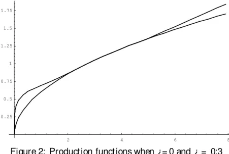
These relationships of F with ¿and pare continuous. The e¤ects of tari¤s on output are illustrated in Figures 1 and 2, for the case where¿ = 0 and ¿ = 1 and the case where¿ = 0and ¿ = 0:3, respectively.

1 2 3 4 5 6

0.25 0.5 0.75 1 1.25 1.5

2 4 6 8 0.25

0.5 0.75 1 1.25 1.5 1.75

Figure 2: Production functions when ¿= 0 and ¿ = 0:3

Note that in the …rst case the curve corresponding to¿ = 0is everywhere (i.e., for any k but k¤_{) above the curve corresponding to¿ = 1 , while in the}

second case there is an interval, [kb1;kb2]; where the curves coincide.

For all values ofpand¿, F is homogeneous of degree one and continuous in K and L. Hence, we can rewrite asy = f (kj¿; p), wherey = Y=L and k = K =L;andf isa continuous function. Generically,f is also locally concave and continuously di¤erentiable, although, if ¿ > 0; global concavity and continuous di¤erentiability is lost becausef 0_{(k) has discrete variations (up}

or down) at the critical values bki.8 This is illustrated in Figures 3 and 4:

for k < kbA; the slope of f 0(k) is negative; it jumps down at kbA and for k 2 [kbA;bk1]; f0(k) is horizontal; it jumps up at kb1 and for k 2 [kb1;bk2] the

slope is negative. After kb2 the curve is horizontal and negative again after

b

kB (not shown in Figure 3).

8_{Not ice however that F is, on the other hand, globally concave and C}1_{if ¿ = 0 (because}

1 2 3 4 5 6

0.16 0.18 0.22

Figure 3: Slope of f(k) when ¿ = 0:1

5 10 15 20

0.14 0.15 0.16 0.17 0.18 0.19

Figure 4: Slope of f(k) when ¿ = 0:3

economy is very di¤erent from the world economy in which the price p is determined.

Now, consider the dynamic problem of an economy with technology F. Usual derivations, assuming log utility, lead to theEuler equationÃ(k; k0_{; k}00_{) =} 0; where

Ã(k; k0_{; k}00_{) = [f (k}0_{) + (1¡ ±)k}0_{¡ (1 + ¹ )k}00_{]¡ (4)}

¯ =(1 + ¹ ) [f (k) + (1¡ ±)k¡ (1 + ¹ )k0_{] [f}0_{(k) + 1¡ ±]}

which characterizes the law of motion ofk. We discuss transitional dynamics in the next section, after providing a quantitative version of the model. For now, we are interested in identifying the set of locally stable balanced growth paths (steady states in k). We know that any balanced growth path will be characterized by a capital-labor ratioke that satis…es

1 + ¹

¯ + ±¡ 1 < f 0₍e_k

¡ ) (5)

1 + ¹

¯ + ±¡ 1 > f 0_(ek

+)

where ke¡ and ke+ are the limits ask ! ~k from below and above. Notice

that (??) is written in this way rather than a single equation since the global concavity off is not guaranteed. In other words, (??) allows for steady states at the critical valueskbi. For the baseline scenario, where we have assumed

that our small country is identical in preferences and technology to the world economy, the following proposition characterizes the set of steady states.

Pr oposit ion 1 For all ¿ > 0 there are two locally stable balanced growth paths. One of them is invariant in ¿, and with capital-labor ratio k¤_{. The}

other one has a lower capital-labor ratio, given by kbA, which is decreasing in ¿.

Proof: First, recall that for all practical purposes the world economy does not trade, and its production function isf¤_{(k) =}

-4k®;the same as our small

economy’s in an interval [kb1;kb2] that containsk¤: Therefore, as k¤ satis…es

( ??) for the world economy, it must also satisfy the same condition for the small economy, and thus constitutes a balanced growth path. Furthermore, one can show that

lim k! bk¡_A

f0_{(k) >} 1 + ¹

which implies that kbA satis…es (??), and is the only balanced growth path in [kbA; k¤) [ (k¤;1 ). Finally, as f0(k) is strictly decreasing in

³ 0;kbA

´

; there are no other balanced growth paths.

Proposition ?? establishes that a small country (identical to the world economy) that starts out poor enough will always fall in a low balanced growth path, (or development trap). For low tari¤ rates, this lower path has a similar k as the world economy, but as tari¤s increase this level of k falls. AsF itself is also decreasing in¿everywhere but at k = k¤_{, output is}

also decreasing in ¿at the development trap, and invariant in¿at the high steady state9_.

This result is then very consistent with the …nding that one cannot statis-tically reject convergence among countries with low barriers to trade, while countries with high barriers tend to stagnate at much lower levels of capital and output, because even if a low-tari¤ economy falls in the trap (converges to the lower steady state), it involves similar inputs (and the same produc-tivity) as the world economy. Meanwhile, when a high-tari¤ country falls in the trap, it is at low levels of inputs and of productivity.

More is learned when one considers also deviations from the baseline sce-nario, allowing di¤erences in preferences or technology. Consider for instance what happens if there are cross-country di¤erences in depreciation rates, or ±6= ±¤_{. On the one hand, if ± < ±}¤_{, then for low tari¤ rates there is a unique}

balanced growth path (with k > k¤_{), while at a high enough tari¤ there are}

two balanced growth paths, one with k higher and one withk lower thank¤_,

and with the lower balanced growth paths decreasing in ¿. In other words, for low tari¤s there is no trap. On the other hand, for ± > ±¤_{, again for}

low tari¤ rates there is a unique balanced growth path, with k < k¤ _and

decreasing in ¿; at higher tari¤s there exist two balanced growth paths.

4 Quant i…cat ion

In this section we try to quantify the order of magnitude of the e¤ects of introducing trade into the basic growth model. For that purpose, we make some modi…cations to the model presented in the last section, and then cal-ibrate the model. With the calcal-ibrated model, we can do numerical exercises

9_{Not ice that …gures 3 and 4 display, below the horizontal axes, the line} 1+ ¹

¯ + ± ¡ 1:

that address three questions regarding the e¤ects of high tari¤s. First, we ask about the size of the productivity decrease. Second, we ask about the rel-ative income at the development traps. Third, we ask about the quantitrel-ative impact on the transitional dynamics towards steady state. The bottom line of all three exercises is that the macroeconomic e¤ects of increasing tari¤s can be important.

Before we address these questions, we modify the model by introducing human capital. It has been argued before (see Mankiw, Romer and Weil (1992) or Chari, Kehoe and McGrattan (1997), for example) that the stan-dard growth models perform much better quantitatively if one allows for this other type of capital; we have done the quantitative analysis both with and without human capital, and con…rmed that this is true here as well. The way we will do this is simply to assume that the …nal good production process uses human capital (denoted H), in the form

Y = £ ³a°_b1¡ °´¾_H1¡ ¾_{: (6)}

It is easy to show that in equilibrium the mapping from factors to output takes the form

Y = G(K ; H ; Lj¿; p) = F (K ; Lj¿; p)¾_H1¡ ¾ ₍₇₎

whereF is the same function de…ned in (??). We give human capital the same law of motion as we gave to physical capital, de…ned in (?? ). The theoretical results found in the previous section still hold in this alternative formulation.

The reader may question whether this is the most reasonable formula-tion. For instance, one may be bothered by the asymmetric treatment of both capitals, asH is only used to make …nal goods whileK is only used to make intermediate goods. As it turns out, we could assume that all fac-tors are used in …nal good production, and still derive (??), (although the formulae for - i would change, of course). Even the calibration would not

change, as we pick the parameters in - i to match gains from trade, rather

a broader physical-and-human capital measure. This clearly does not a¤ect the qualitative results, and in fact yields similar quantitative results.

We now calibrate the model. Recall that, in the larger world economy, the equilibrium determination of …nal good output per unit of labor isy = £k®¾_h1¡ ¾_{. We interpret that economy to be the US (or the US plus other}

rich countries). Then, we can pick parameters as to mimic the calibration of real business cycles, closed economy models for the US that is common in the literature. That leads us to pick the parameters±, ¹ and ¯ that would generate without trade a2%per-capita growth,6:1%net return on capital, and a2:75physical capital to annual output ratio along the balanced growth path. The shares of human and physical capital are conventionally picked to

be®¾= 1¡ ¾= 1=3.

For lack of information on the parameter °, we opt for symmetry and chose the value1=2. The chosen value of ° does not a¤ect the results much, provided that one adjusts the other parameters to maintain the calibration of ®and¾. The valueof£ is selected as to normalize, without loss of generality, tok¤_{= h}¤_{= 1; under that normalization and given ° = 1=2; it follows that} p = 1:

This pins down the average ® of the two parameters ®a and ®b, but

leaves freedom of choosing one of them. The choice of these two parameters is important, as the quantitative e¤ects of all trade-related phenomena are bound to be larger the spread ®b¡ ®a is, leaving®constant.10 One way to

discipline the choice of parameters is by choosing ®a and ®b conservatively

to match the relatively small estimations in the literature about the size of gains from trade in rich countries.11 _{Our baseline choice will be®}

a = 0:42

and ®b = 0:58. With those values, the model predicts that the total static

gains from trade, interpreted as the total di¤erence in …nal good output associated with comparing ¿ = 0 with ¿ = 1 , are less than 1% of GDP for any country with 75%or more of US output per worker (the world´ s 18 wealthiest countries). The parameters also imply that total static gains from

10_{For instance, Ventura (1997) demonst rates that one can even get endogenous growth}

by assuming ®a = 0, ®b = 1. On t he ot her hand, there is no trade at all under any

circumstances if ®a = ®b.

11_{As an example, Kehoe and Kehoe (1994) est imat e the e¤ect of NAFTA to be very}

trade (that is, the whole output di¤erence in going from¿ = 1 to¿ = 0) are only 4:8%of GDP for a country with Mexico´ s income, and only9%of GDP for countries, like Brazil or Costa Rica, with roughly a third of US output per worker.

Under those parameters, consider …rst the static e¤ect of tari¤s on mea-sured productivity. Why do tari¤s reduce productivity? For two reasons, both completely standard within the Hecksher-Ohlin model of international trade. First, they distort the prices used in the decision of how to allocate the factorsK andL between the intermediate goods production, a distortion that reduces the value of national product at international prices. Second, the same price distortion a¤ects the ratio of the two intermediate inputs used by the …nal good producers, as the relative price they see, q, is not the same as the actual opportunity cost posed by the international market, which is the pricep.

Figure 5 shows proportionately how much higher would productivity be with ¿ = 10% than with ¿ = 40%, as a function of the stock of physical capital, given human capital. We can see that, while for rich enough countries the di¤erence is negligible, for the very poor countries these two policies yield a di¤erence in productivity of around 9%.

0.3 0.4 0.5 0.6 0.02

0.04 0.06 0.08 0.1

Figure 5: Productivity di¤erences as function of inputs³ ¿= 10% ¿= 40%

´

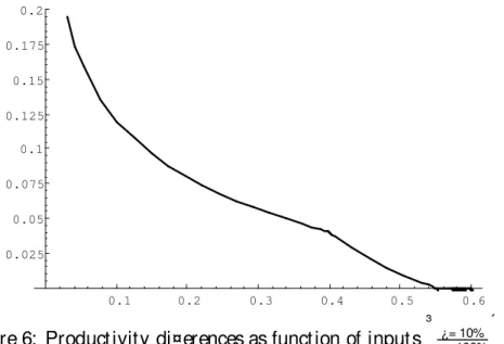
(estimates of the e¤ective rate of protection for many developing countries in the 70’s and 80’s are around 100%). Now, the e¤ects in productivity are about twice as large. In a closed-economy model, these di¤erences in mea-sured productivity would go unexplained. It is not surprising that empirical studies …nd a cross-country relationship between tradebarriers and measured TFP.

0.1 0.2 0.3 0.4 0.5 0.6 0.025

0.05 0.075 0.1 0.125 0.15 0.175 0.2

Figure 6: Productivity di¤erences as function of inputs³ ¿= 10% ¿= 100%

´

We now study the magnitude of the development traps presented in Proposition 1. We focus on the case where there is no di¤erence in pa-rameters between the world economy and our small economy, which means that both have a high steady state with the same input and output levels. What we ask is how big are the di¤erences between the two steady states (between an economy that has fallen in the trap and one that has converged to the higher balanced growth path), and the sensitivity of those di¤erences to trade protection.

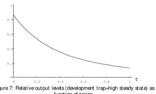
0 0.2 0.4 0.6 0.8 1 τ 0.2

0.4 0.6 0.8 1

Figure 7: Relative output levels (development trap=high steady state) as function of tari¤s.

This result is consistent with the empirical work mentioned in the intro-duction, which found that inputs, and not only productivity, are a¤ected by trade protection. In fact, the cross-country di¤erences in output that one can generate with realistic tari¤ rates are fairly large, since countries with 100% e¤ective rates of protection are, unfortunately, not rare. The observed income di¤erences accros countries can thus be explained as being caused by the the dispersion of trade policies in the recent past, as re‡ect by di¤erences in tari¤s but also by their non-tari¤ equivalents such as quotas and import bans.

Finnaly, consider now the e¤ects of trade on the transitional dynamics to the balanced growth path. To see this, we solve the dynamic problem posed by (??), using Coleman’s policy function iteration, for the cases where ¿ = 0and¿ = 1 .12 _{We then generate simulated transition paths, for various}

initial conditions, using the policy functions for the two tari¤ choices. We are interested in comparing the di¤erence in output and the di¤erence in

12_{Because for ¿ = 0 and ¿ = 1 t he production function is globally concave and C}1 _we

consumption between the open economy path and the closed economy path, at each point in time, assuming the same initial level of H and K =L.

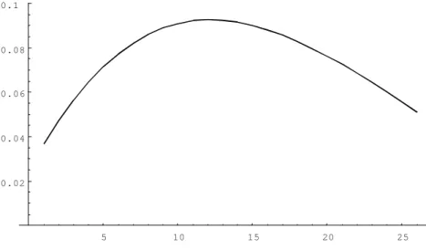
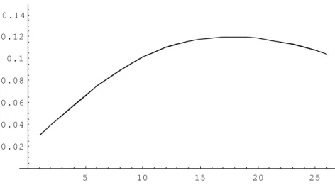
Due to thestatic gains mentioned above, even at the initial (and common) levels of k and h there is a gap between the open and closed economies. If the initial condition is at a low level ofhandk, we also see the open economy accumulate factors faster, and thus amplify the di¤erence in output over its closed-economy counterpart as time goes by. Over the …rst few years, the output di¤erence becomes much larger; for many initial conditions it gets to be 3 times or more than the original productivity di¤erence. As time goes by, however, the closed economy begins to catch up and eventually overtake. Figures 8 and 9 illustrate the di¤erences in the transition. It is drawn for a case where the initial stocks of both capitals are at around6%of their steady state values.

5 10 15 20 25

0.02 0.04 0.06 0.08 0.1

5 10 15 20 25 0 . 0 2

0 . 0 4 0 . 0 6 0 . 0 8 0.1 0 . 1 2 0 . 1 4

Figure 9: Consumption di¤erences during the transition path

5 Conclusion

In this paper, we have studied a model that integrates a simple comparative-advantage trade model (the Hecksher-Ohlin model) in an dynamic optimal growth model. The main theoretical results are that barriers to international trade reduce the total factor productivity of an economy and, more impor-tantly, can cause the existence of development traps, or low-income steady states. We then calibrate the model, to get an idea of the possible order of magnitude of the e¤ects of trade policy on macroeconomic performance. We …nd that the aggregate e¤ects of trade barriers can be large, in productivity, in speed of convergence, and in long run output.

A

T he pr oduct ion funct ion

In the appendix we present in details the derivation of the production func-tion used in the paper. After presenting general properties of the model we derive the production function for the closed economy case, then for the case of an open economy with no tari¤s and …nally the most relevant case, the open economy with positive tari¤s.

The production function for the two intermediate products, a and b, is given by:

A = K®a

A L1 ¡ ®A a and B = KB®bL1 ¡ ®B b

Total production of the …nal good is given by

Y = a°_b1 ¡ ° ₍₈₎

whereaand bare the total inputs used of the two intermediate products. In the closed economy, these inputs have to be locally produced, so the economy is constrained by a = A; b = B ;while in the open economy trade is possible, yet we do not allow external debt , and so the constraint is

pa + b = pA + B

where p is, of course, the international price of A relative toB, which we will assume that our economy takes as a parameter. We assume that …nal goods are not tradable. They are consumable and investable. It is useful to get Y as a function of K and L, taking the equilibrium A; B ; a; bimplicitly. We know that in the closed economy, the planner maximizes

³ K®a

A L1 ¡ ®A a

´_° h

(K ¡ KA)®b(L ¡ LA)1 ¡ ®b

i_{1 ¡ °}

First order conditions are given by

°(1¡ ®a) LA

= (1¡ ° ) (1¡ ®b) (L ¡ LA) ° ®a

KA

= (1¡ ° ) ®b

(K ¡ KA)

which yield

LA = °

1¡ ®a

KA = ° ®a: K

° ®a+ ®b¡ ®b°

LB = L (1¡ ®b)

1¡ °

1¡ ° ®a¡ (1¡ ° )®b

KB = K ®b

1¡ ° ° ®a+ ®b¡ ®b°

So that output under autarky is given by

Y = °°_{(1¡ ° )}1 ¡ °_¡K®a° + ®b(1¡ ° )L( 1 ¡ ®a)° + (1¡ ®b)(1¡ ° ) (9)

where

¡ = [®®aa(1¡ ®a)1 ¡ ®a]°[®®bb(1¡ ®b)1 ¡ ®b]1¡ °

[1¡ ° ®a¡ (1¡ ° )®b]1¡ ° ®a¡ (1¡ ° )®b[° ®a+ (1¡ ° ) ®b]° ®a+ (1¡ ° )®b

The relative price of A in autarkic equilibrium becomes

®_bK®b¡ 1

b L1¡ ®b b ®_aK®a¡ 1

a L1¡ ®a a = p¤

which in equilibrium becomes

®®b

b (1¡ ®b)1¡ ®b ®®a

a (1¡ ®a)1¡ ®a

"

K =[° ®a+ ®b¡ ®b° ] L=[1¡ ° ®a¡ ®b+ ®b° ]

#

= p¤ ₍₁₀₎

The capital-labor ratio corresponding top¤ _isk¤_:

For the case where0< ¿ < 1 there are …ve relevant cases. First, the country could produce only a, onlybor be diversi…ed; then, when diversi…ed, it could be exportinga, exportingbor not trading and at the closed economy solution written above.

The economy will be in autarky whenever

p > p¤_{> p=(1 + ¿) or when p < p}¤_{< p (1 + ¿)}

because it loses the comparative advantage it has in goodaor b;respectively. In that event the production function is given by the closed economy solution written above (equation [??]).

tau is equal zero), we have to work out in two stages. In the …rst one the factor allocation and intermediate production of a and bis determined and Q = pa + bis de…ned: In the second stage, the demand for aand bgiven Q is solved.

The demands for aandb, satisfy

pa + b = Q and °

1¡ ° b a =

p 1 + ¿

Solving for theseequationsand substituting into the…nal good production function (eq. ??), we get:

Y = °° _{(1¡ ° )}1¡ ° _p1¡ °_Q(1 + ¿) °

1 + ° ¿ (11)

To obtain Q note that there is a bound pza such that if p > pza, thenQ

corresponds to the value of potential aoutput. In this caseQ = pK®a

A L1 ¡ ®A a

and then:

Y = °° _{(1¡ ° )}1¡ ° _p1¡ °_K®a_L1 ¡ ®a(1 + ¿)

°

1 + ° ¿ (12)

Whenp < pza the economy is diversi…ed in intermediate good production

and thenQ = pa + b; whereaandbare the solutions to the factor allocation problem. In other words, we solve for the maximands of

p 1 + ¿K

®a

A L1¡ ®A a + (K ¡ KA)®b(L ¡ LA)1¡ ®b (13)

Assuming there are no restrictions on the inputs for each sector, uncon-strained maximization of the above expression yields :

KA LA

= "

p 1 + ¿

µ_®

a ®b

¶_®bµ_{1¡ ®}

a 1¡ ®b

¶1¡ ®b# 1 ®b¡ ®a

= s1 (14)

K ¡ KA

L ¡ LA =

" p 1 + ¿

µ_®

a ®b

¶_®a µ_{1¡ ®}

a 1¡ ®b

¶1¡ ®a#_{®b¡ ®a}1

= s2

Notice that, under the assumption that bis the capital intensive good

s2 s1 = µ_® b ®a

¶ µ_{1¡ ®}

a 1¡ ®b

¶ > 1

KA = s1LA

K ¡ KA = s2(L ¡ LA)

imply

LA = x_x2₂L ¡ K_{¡ x1} LB = K ¡ x_{x2¡ x}1₁L

KA = x1x_x2₂L ¡ K_{¡ x1} KB = x2K ¡ x_{x2¡ x}1₁L

Under these inputs, then, total Q is given by :

Q = Lps ®a

1 s2¡ s®2bs1 s2¡ s1

+ K s

®b

2 ¡ ps®1a s2¡ s1

Plugging the above expression in equation (??) we obtain:

Y = °° _{(1¡ ° )}1¡ ° _p¡ °(1 + ¿) °

1 + ° ¿ "

Lps ®a

1 s2¡ s®2bs1

s2¡ s1 + K

s®b

2 ¡ ps®1a s2¡ s1

#

(15)

Finally,pza comes from the expression of s1 :

µ_K

L

¶®b¡ ®aµ _®

b ®a

¶_®bµ _{1¡ ®}

b 1¡ ®a

¶1¡ ®b

(1 + ¿) = pza

The capital-labor ratio corresponding topza iskba .

For the case where the country exercises comparative advantage inb(that is, p¤_{> p(1 + ¿) demand for aandbhas to satisfy:}

pa + b = Q and °

1¡ ° b

a = p (1 + ¿)

Solving for theseequationsand substituting into the…nal good production function, we get:

Y = °° _{(1¡ ° )}1¡ ° _p¡ °_Q (1 + ¿)1¡ ° 1 + (1¡ ° ) ¿

Again there are two relevant sub-cases here. There is apzb such that if p < pzb the economy only producesb; and then:

Y = °° _{(1¡ ° )}1¡ °

p¡ ° (1 + ¿) 1¡ °

1 + (1¡ ° ) ¿K

®bL1 ¡ ®b (16)

On the other hand, if p¤

(1+ ¿) > p > pzbboth goods will be produced and we

(K ¡ KA)=(L ¡ LA) = z2 similar to (??) but, again, with p(1 + ¿) instead

of p=(1 + ¿) : These expressions, after some manipulations, will give us:

Y = °° _{(1¡ ° )}1¡ ° _p¡ ° (1 + ¿) 1¡ °

(1 + (1¡ ° ) ¿) "

Lpz ®a

1 z2¡ z2®bz1 z2¡ z1

+ K z

®b

2 ¡ pz®1a z2¡ z1

#

(17) Finally, pzbcomes from the expression of z2 :

µ K

L

¶®b¡ ®aµ_®

b ®a

¶_®aµ

1¡ ®b 1¡ ®a

¶1¡ ®a ₁

(1 + ¿) = pzb

The capital-labor ratio corresponding topzbisbkb.

We have already de…ned all …ve segments of function F (K ; Lj¿; p)( eq. [3.1]):

1. for K =L < bkA; F (K ; Lj¿; p) is given by eq. (??) and - 1 corresponds

to°° _{(1¡ ° )}1¡ ° _p1¡ ° _{(1 + ¿)}° _{=(1 + ° ¿):}

2. For K =L > bkB; it is given by eq. (??) and - 7 corresponds to°°(1¡ ° )1¡ ° _p¡ ° _{(1 + ¿)}1¡ ° _{=[1 + (1¡ ° )¿]:}

3. If K =L 2 [kbA;kb1]( kb1 being the capital-ratio which corresponds to p¤_{[1 + ¿]), then F (K ; Lj¿; p) is given by eq.(??),}

-2 corresponding to - 1[s®2b ¡ ps1®a]=[p(s2¡ s1)] and - 3 to- 1[ps®1as2¡ s2®bs1]=[p(s2¡ s1)]:

4. For the case whereK =L 2 [kb1;kb2]( kb2 being the capital-ratio which

corresponds top¤_{=[1+ ¿]), the expressions for}

-5 and- 6are symmetric

to - 2 and - 3, with - 7 substituting- 1 and z1 and z2 substituting s1

and s2;respectively.

5. Finally, when K =L 2 [kb1;kb2] the economy is closed and F (K ; Lj¿; p)

corresponds to eq. (??) and - 4 is given by °°(1¡ ° )1 ¡ °¡:

For the case where¿ = 0;we have only 3 relevant cases, askb1 andkb2

col-lapse tok¤_{: 1) The economy specializes in gooda; 2) The economy specializes}

in good b;3) The economy diversify. In the latter case the production func-tion is linear on K and L while for the other two it will be Cobb-Douglas with coe¢ cients ®a and ®b; respectively. The economy will always trade,

Refer ences

[1] Chari, V., Kehoe, P. and E. McGrattan(1997) The Poverty of Nations: A Quantitative Exploration, FRB of Minneapolis Research Department Sta¤ Report 204.

[2] Corden, W. (1971) The e¤ects of trade on the rate of growth. in Bhag-wati, Jones, Mundell e Vanek, Trade, Balance of Payments and Growth, North-Holland, pp. 117-143.

[3] Dixit, A.K. and V. Norman (1980) ” Theory of International Trade,” Cambridge University Press, Cambridge, MA.

[4] Edwards,S.(1993) ” Openness, Trade Liberalization and Growth in De-veloping Countries,” Journal of Economic Literature, 31, 3. pp. 1358-1393.

[5] Edwards, S. (1997)” Openness, Productivity and Growth: What do we Really Know?” , NBER working paper # 5978.

[6] Frankel, D., and D. Romer(1996) ” Trade and Growth: an Empirical Investigation,” NBER working paper 5476.

[7] Grossman, G. e E. Helpman(1991) ” Small Open Economy,” in Innova-tion and Growth in the Global Economy, pp. 144-176, MIT Press.

[8] Hall,R. and C. Jones(1999) ” Why Do Some Countries Produce so Much More Output per Worker than Others?,” Quarterly Journal of Eco-nomics, February, Vol. 114, pp. 83-116.

[9] Harrison, A. (1995) ” Openness and Growth: a Time-Series, Cross-Country Analysis for Developing Countries,” NBER Working Paper No. 5221.

[10] Holmes, T., e J. Schmitz Jr.(1995) ” Resistance to New Technology and Trade Between Areas,” FRB of Minneapolis Quarterly Review, winter, pp. 2-18

[12] Krueger, A(1997) ” Trade Policy and Economic Development: How we Learn.” American Economic Review, 87, pp. 1-22.

[13] Lee, J.W. (1996) ” Government Interventions and Productivity Growth,” Journal of Economic Growth, v1(3), 391-414.

[14] Mankiw, G., Romer, D. and D. Weil(1992) ” A Contribution to the Em-pirics of Economic Growth,” Quarterly Journal of Economics, 107, 2, pp. 407-437.

[15] Parente, S. and E.C. Prescott(1994), Barriers to Technology Adoption and Development, Journal of Political Economy, v.102(2), 298-321.

[16] Prescott, E.C.(1998), ” Needed: a Theory of Total Factor Productivity,” Federal Reserve Bank of Minneapolis Sta¤ Report # 242.

[17] Quah, D. (1996) ” Twin Peaks: Growth and Convergence in Models of Distributional Dynamics,” Economic Journal, Vol. 106, July, pp. 1045-55.

[18] Rebelo, S. (1991) ” Long Run Analysis and Long-Growth,” Journal of Political Economy, 99, 3, pp. 500-521

[19] Riviera-Batiz, L. A. and P. Romer (1991) ” Economic Integration and Endogenous Growth” - Quarterly Journal of Economics, Vol. 106(2), 531-556.

[20] Rodriguez, A (1996) ” Multinationals, Linkages, and Economic Develop-ment,” American Economic Review; 86(4), September, pp. 852-73.

[21] Sachs, J. and A. Warner(1995) ” Economic Convergence and Economic Policies,” NBER working paper # 5039.

[22] Stiglitz, J. (1998) More Instruments and Broader Goals: From Washing-ton to Santiago,” Mimeo, Academia de Centroamerica, San Jose, Costa Rica.

[24] Taylor, A. (1996) ” On the Cost of Inward-Looking Development: Price Distortions, Growth and Divergence in Latin America,” Mimeo, North-western University.

[25] Trejos, A. (1992) ” On the Short-Run Dynamic E¤ects of Comparative Advantage Trade,” Mimeo, University of Pennsylvania.

[26] Ventura, J.(1997), ” Growth and Interdependence” Quarterly Journal of Economics; 112(1), February 1997, pp. 57-84.