Reconstructing triangulated surfaces from unorganized points through local skeletal stars

(1)

Engenharia

Reconstructing Triangulated Surfaces from

Unorganized Points through Local Skeletal Stars

Tiago Branco Pereira

Dissertação para obtenção do Grau de Mestre em

Engenharia Informática

(2º ciclo de estudos)

Orientador: Prof. Doutor Abel João Padrão Gomes

(2)

(3)

(4)

(5)

Acknowledgements

With no doubt, this project was the biggest and most changeling project I have ever done. But it wasn’t possible to me to finish it, without the help of some people, who helped me in this progress, and its my duty to thank them all.

First of all, I want to express my gratitude to my supervisor, Prof. Abel Gomes. Without him this journey would not have come to an end.

Secondly, I also what to thank Orlando, who helped me, heard me in difficult times and for his advices.

Last but not least, I wasn’t here without the help and hard work of my parents. Their spirit of sacrifice and love will be never forgotten. A gigantic Thank you.

(6)

(7)

Resumo

Reconstrução da superfície de pontos desorganizados surge em uma variedade de situações práti-cas, tais como rastreamento de um objeto a partir de vários pontos de vista, a recuperação de formas biológicas de fatias bi-dimensionais, e esboçar superfícies interativas.

O algoritmo apresentado nesta dissertação tem como entrada um conjunto desorganizado de pontos{x1, ..., xn} ⊂ R3em um coletor desconhecido M , e produz como resultado uma superfície

simplicial que se aproxima de M , enquanto a única informação conhecida é as coordenadas (x, y, z)dos pontos.

Um conjunto de regras são aplicadas para cada um dos pontos para determinar uma malha-esqueleto inicial. Este malha-esqueleto vai ter as informações de topologia do objeto, dando infor-mações da próxima conectividade no processo de crescimento da malha, ou seja, ele tira a necessidade de pesquisa dos pontos que se vão ligar à fronteira.

Palavras-chave

Amostra Computação Geometrica Reconstrução da Superfície Malha Triangular Nuvem de Pontos Crescimento da Malha

(8)

(9)

Abstract

Surface reconstruction from unorganized points arises in a variety of practical situations such as range scanning an object from multiple view points, recovery of biological shapes from two-dimensional slices, and interactive surface sketching.

The algorithm presented in this dissertation takes as input an unorganized set of point{x1, ..., xn} ⊂

R3_{on an unknown manifold M , and produces as output a simplicial surface that approximates} M, while the only information known are the (x, y, z) of the points.

A set of rules are applied for each of this points to determine a initial skeleton mesh. This skeleton will have the topology information of the object while giving information of next con-nectivity in the process of mesh growing, i.e it takes away the require of search of the edge points.

Keywords

Sampling Computation Geometry Surface reconstruction Triangle mesh Point Cloud Mesh Growing

(10)

(11)

List of Figures

3.1 (a) Corrugated Cloud Point; (b) Corrugated Mesh. . . 17

3.2 Side view of a corrugated Mesh . . . 17

3.3 Mesh with abrupt changed of point density . . . 18

3.4 Abrupt variance of point density . . . 18

3.5 Point Density (top view of the mesh) . . . 21

3.6 Very sharp curves (2D view of a side cut of the mesh) . . . 21

3.7 Sem a aplicação da regra (left); Ângulos maiores que 30º (right). . . 22

3.8 Sem a aplicação da regra (left); Ângulos maiores que 30º (right). . . 23

3.9 Vector normal usando eigenvector a azul (left). . . 24

3.10 Cálculo das normais . . . 26

3.11 Descrição da Imagem . . . 27

3.12 Attempt to create triangle q1pq2 . . . 28

3.13 Attempt to create triangle q1pq2 . . . 29

3.14 Cloud Point of the Object . . . 30

3.15 Pre-Mesh of a Sub-set of points from the Object . . . 31

3.16 Triangulated Sub-set of point from the Object . . . 31

3.17 Pre-Mesh of a Sub-set of points from the Object . . . 32

3.18 Triangulated Sub-set of point from the Object . . . 32

3.19 Skeleton mesh . . . 33

3.20 Triangulated Mesh without triangles . . . 33

3.21 Triangulated Mesh with triangles . . . 34

3.22 Skeleton mesh . . . 34

3.23 Triangulated Mesh without triangles . . . 35

(14)

(15)

List of Tables

(16)

(17)

List of Abbreviations

3D Three dimensional

(18)

(19)

Chapter 1

Introduction

Surface Reconstruction is a challenging problem in the field of computer graphics with a wide

range of application areas like medical imagery, virtual reality, video games, movies, e-commerce and other graphic applications. The unorganized point clouds derived from varied inputs like laser scanner data, photogrammetric image measurements, motion sensors etc. pose a tough problem of reconstruction, not completely solved and challenging in case of incomplete, noisy and sparse data.

1.1 Thesis Statement

With this grand challenge mentioned above in mind, the core of this dissertation is the following: The goal of surface reconstruction is to determine a surface S from a given set of points P , sampled from a surface in R3_{such that the points of set P lie on S. The surface S approximates}

the set of points P . From a mathematical point of view, a surface in the Euclidean three-dimensional space R3_{is defined as a two-dimensional manifold that is compact, connected and}

contains information about face orientation. In other words, we might say that a surface is a “continuous” subset of points in R3_{which is locally two-dimensional.}

1.2 Motivation

The reconstruction of satisfactory models which can fulfill the high modeling and visualization demands of such application areas is a nontrivial problem which has not been completely solved because of incomplete, noisy and spare input data at hand. The raw input points are often unorganized, lacking inherent structure or orientation information.

Surface reconstruction from raw geometric data has received increasing attention due to the ever broadening range of geometric sensors, laser data scanners and vision algorithms that provide little to no reliable attributes. The unavoidable presence of noise and outliers makes the challenge even greater and any progress in this direction can also directly benefit reconstruction from point data set input or the point clouds with attributes. The goal is to create the model of an object which best fit the reality. Polygonal meshes are the commonly accepted graphic representation, with the widest support from existing software and hardware.

The wide range of applications from which the data may emerge (e.g. manufacturing, reverse engineering, cultural heritage, architecture) implies that the data can have quite different properties that must be considered in the solution of the surface interpolation problem. The goal is always to find a way to create a computer model of an object which best fit the reality. Polygons are usually the ideal way to accurately represent the results of measurements,

(20)

providing an optimal surface description. While the generation of digital terrain models has a long tradition and has found efficient solutions, the correct modeling of closed surfaces or free-form objects is of recent nature, a not completely solved problem and still an important issue investigated in many research activities.

1.3 Problem Statement

The problem stated in this dissertation is that when object are only known by three coordinates (x, y, z) of a set of points selected on the boundary of the object (know as Cloud Points). There is no relation between any sub-set of points, thus, it has no topologic information about the object. So for a object O, let S be the surface embedded in Euclidean 3D space R3_{, and given}

a set of points P, pi∈ P ⊂ R3, i = 1, ..., N, that samples surface S, it is required to find surface

S′ that approximates S. In the end surface S′need to be topologically equivalent to surface S of the original object.

1.4 Important Terms

• Mesh: it is a collection of triangular (or quadrilateral) contiguous, non-overlapping faces joined together along their edges. A mesh therefore contains vertices, edges and faces. • Surface: a compact, connected, orientable 2D or 3D manifold, possibly with boundary. A

surface without boundary is a closed surface. A surface can be geometrically represented in implicit form (locus of the solution of the function F (x, y, z) = 0) or parametric form. • Open GL: OpenGraphics Library is cross-language, multi-platform application programming

interface (API) for rendering 2D and 3D computer graphics.

• Mesh Drifting: When two meshes are too close to each other, therefore points from one mesh have as its closest point from the other mesh.

1.5 Software and Hardware Tools

In terms of software development, all the code was exclusively and fully designed and written by the author. Every function presented in this dissertation was written in C++ and OpenGL. The development environment used were Xcode. No special hardware like parallel or high-performance computers, or even high high-performance graphics cards, were used at all, just a regular laptop computer.

1.6 Organization of the Thesis

(21)

• Chapter 1 contains an introduction to the dissertation. This chapter also introduces the thesis statement.

• Chapter 2 presents the state-of-the-art in Surface Reconstruction. • Chapter 3 presents a new method of simplicial surface reconstruction. • Finally, Chapter 4 presents the final conclusions for this dissertation.

(22)

(23)

Chapter 2

State-of-the-art in Surface Reconstruction

Surface reconstruction has become an important research topic in part due to the appearance of 3D range scanners on the market. These scanners are capable of acquiring unstructured 3D point datasets from the surface of a given physical object. Digital scans allow for high-quality surface reconstructions, but this requires a particular care in recovering sharp features such as ridges, corners, spikes, etc. Surface reconstruction has many applications in science and engineering, in particular, geometric modelling, computer graphics, virtual reality, computer animation, computer vision, computer-assisted surgery, and reverse engineering.

2.1 Introduction

This chapter deals with surface-fitting algorithms that reconstruct surfaces from clouds of points. There are several surface reconstruction techniques depending on the representation in hand: simplicial, parametric, implicit surfaces. Even though they are different representations, they share various issues and problems. This chapter starts with a brief review on these surface reconstruction techniques, after which the focus will be on the mesh-growing ones.

2.2 Classification of Reconstruction Algorithms

In the literature, there are three main classes of reconstruction algorithms: simplicial surfaces, parametric surfaces, and implicit surfaces.

2.2.1 Simplicial Surfaces

Sometimes, simplicial surfaces are also called triangulated surfaces. There are two main classes of techniques to reconstruct simplicial surfaces from a scattered set of points: Delaunay-based and region-growing techniques. With Delaunay-based approach, we end up having a space parti-tioning into tetrahedra. To be more specific, the typical Delaunay-based surface reconstruction algorithm consists of two steps:

• Delaunay triangulation. First, one constructs the Delaunay triangulation (or Voronoi di-agram) from such a cloud of points, which consists of a partition of the convex hull of these sample points into a finite set of tetrahedra. The main advantage of the Delaunay triangulation comes from its uniqueness; it is unique if no five sample points can be found on a common sphere. Several algorithms for constructing a Delaunay triangulation can be found in the literature, in particular those given by Bowyer[Bow81], Watson [Wat81], Avis

(24)

and Bhattacharya [AB83], Preparata and Shamos [PS85], Edelsbrunner [Ede87], and, more recently, Hjelle and Dæhlen [HD06], just to mention a few.

• Triangulated surface extraction.Terminated the triangulation of the cloud of points, it only remains to identify which simplices belong to the surface. Thus, the reconstruction of simplicial surfaces consists in finding the subgraph of Delaunay triangulation of the initial set of points [EM94]. The identification of surface simplices varies from an algorithm to another.

The first Delaunay-based surface reconstruction method seems to be due to Boissonnat [Boi84]. In the class of Delaunay-based surface reconstruction methods, we also find the α-shapes of Edelsbrunner and Mücke [EM94], the crust and the power crust algorithms of Amenta et al. [ABK98, ACDL02, ACK01], the co-cone algorithm of Dey et al. [DGLW01, DG03], and more re-cently the reconstruction algorithms due to Yau et al. [KY03, YKY02]. Amongst these algorithms, the algorithm of Yau et al. [KY03] preserves sharp features, but only in convex regions, while the algorithm of Amenta et al. [ACK01] is capable of reconstructing sharp edges and corners by steering poles, a subset of circumcentres of tetrahedra. In both cases, multiple Delaunay computations are required, so that the corresponding reconstruction algorithms are rather time-consuming to use.

The second class of algorithms to reconstruct simplicial surfaces is based on the concept of continuation. In the context of surface reconstruction, continuation algorithms are known as region-growing algorithms. Starting from a seed triangle, say initial region, the algorithm iter-ates by attaching new triangles to the region’s boundaries. The early surface-based algorithm due to Boissonnat [Boi84], the graph-based algorithm of Mencl and Müller [MM98], the ball-pivoting algorithm of Bernardini et al. [BMR+_{99a], the projection-based triangulating algorithm}

of Gopi and Krishnan [GK02], the interpolant reconstruction algorithm of Petit- jean and Boyer [PB01], the advanced-front algorithm of Hung and Menq [HM02], and the greedy algorithm of Cohen-Steiner and Da [CSD04], all fall into the class of region-growing algorithms.

In the literature, we also find hybrid algorithms that combine Delaunay- based and region-growing approaches; for example, the algorithm of Kuo and Yau [KY03, KY05] is a representa-tive of these hybrid algorithms. These algorithms were later improved in order to reconstruct surfaces with sharp features [KY06].

2.2.2 Parametric Surfaces

Parametric surface fitting algorithms, also called spline-based surface reconstruction algorithms, are quite common in numerical analysis and computer graphics. In the context of parametric representations, the problem of surface reconstruction involves the computation of a surface S that approximates as much as possible each point of a given cloud of points inR3_{. The goal is}

then to find a parametric surface S, defined by a function F (u, v), that closely approximates a given cloud of points, where F belongs to a specific linear space of functions. Examples of such parametric surfaces are Bézier and B-spline surfaces [Far97].

Traditionally, the parametric surface reconstruction algorithm consists of four main steps, namely: • Mesh generation from the unorganised point cloud. This can be done by, for example, using

(25)

further references), and α-shapes [EM94].

• Mesh partitioning into patches homeomorphic to disks. These patches are also known as charts. The surface mesh partitioning becomes mandatory when the surface is closed or has genus greater than zero. Roughly speaking, there are two ways of cutting surfaces into charts: segmentation techniques and seam generation techniques. For parametrisation purposes, segmentation techniques divide the surface into several charts in order to keep as short as possible the parametric distortion resulting from the cuts. Unlike segmentation, seam cutting techniques are capable of reducing the parametric distortion without cutting the surface into separate patches. For that purpose, they use seams (or partial cuts) to reduce a surface of genus greater than zero to a surface of genus zero. For more details about surface mesh partitioning, the reader is referred to Sheffer et al. [SPR06] and the references therein.

• Parametrisation. For each mesh patch, one constructs a local parametrisation. These local parametrisations are made to fit together continuously such that they collectively form a globally continuous parametrisation of the mesh. In computer graphics, this method was introduced by Eck et al. [EDD+_{95], who used harmonic maps to construct a (local)}

parametrisation of a disk over a convex polygonal region. Nevertheless, before that, Pinkall and Polthier had already used a similar method for computing piecewise linear minimal surfaces [PP93]. For more details on this topic, the reader is referred to Floater and Hormann [FH05] and the references therein.

• Surface fitting. Terminated the parametrisation step, which outputs a collection of pairs of parameters (ui, vi)associated to the points (xi, yi, zi)of the cloud, it remains the

prob-lem of surface fitting. Surface fitting consists in minimising the distance between each point (xi, yi, zi)and its corresponding point of the surface F (ui, vi).

The standard approach of surface fitting reduces to the following minimisation problem:

min∑||xi− F (ui, vi)||2 (2.1)

where xi is the ith input cloud point (xi, yi, zi)and|| · || is the Euclidean distance between xi

and the corresponding point on the surface F (ui, vi) in the above mentioned linear space of

functions. The objective function of this minimisation problem is then the squared Euclidean norm. Its computation can be done easily by the least squares method; hence the least-squares (LS)fitting for parametric surface reconstruction [CRE01, Far97]. As argued in [PL03], this is the main approach to approximating an unstructured cloud of points by a B-spline surface. Alternatives to LS fitting using parametric surfaces are:

• Active contours. This approximation approach is borrowed from computer vision and im-age processing, and is due to Kass et al. [KWT88] who introduced a variational formulation of parametric curves, called snakes, for detecting and approximating contours in images. Since then various variants of snakes or active contours have appeared in the literature [BI98]. In the context of parametric surface reconstruction, the active contour technique was introduced by Pottmann and Leopoldseder [PL03], which uses local quadratic approx-imants of the squared distance function of the surface or point cloud to which we intend

(26)

to fit a B-spline surface. Interestingly, this approach avoids the parametrisation problem, i.e. the third step of the standard procedure described above.

• Lp fitting. The use of Lp norms in fitting curves and surfaces to data aims at finding a

member of the family of surfaces inRn _{which gives a best fit to N given data points.}

The least squares or L2norm is just an example of a fitting technique that minimises the

orthogonal distances from the data points to the surface. Note that the least squares norm is not always adequate, in particular when there are wild points in the data set. This leads us to look at other Lp norms for surface fitting [AW04]. For example, Marzais and

Malgouyres [MGM06] uses a linear programming fitting which is based on the L_∞ norm, also called the uniform or Chebyshev norm. The L_∞fitting outputs a grid of control points of a parametric surface (e.g. Bézier or B-spline surface).

2.2.3 Implicit Surfaces

Most implicit surface reconstruction algorithms from clouds of points are based on Blinn’s idea of blending local implicit primitives [Bli82], called blobs. This blending effect over blobs fits the requirements of modelling a molecule from an union of balls that represent atoms. Muraki [Mur91] combines Gaussian blobs to fit an implicit surface to a point set. Lim et al. [LTGS95] use the blended union of spheres in order to reconstruct implicit solids from scattered data; the spheres are obtained from a previous configuration of spheres given by the Delaunay tetrahe-dralisation of the sample points.

In computer graphics literature, in 1987, Pratt [Pra87] was who first called attention to fitting implicit curves and surfaces to data, since parametric curves and surface had received the most attention in the fitting literature, creating the misleading idea that implicit curves and surfaces are less suitable for fitting purposes. Also, Pratt affirms that none treatment of least squares fitting of implicit surfaces to data was found in the literature. In 1991, Taubin [Tau91] noted that there was no previous work on fitting implicit curves in 3D, having found only a few references on fitting quadric surfaces to data in the literature of pattern recognition and computer vision. Since then, two major classes of implicit fitting methods have been introduced in the literature:

• Global methods. These methods aim to construct a single function such that its zero set interpolates or approximates the cloud of points globally.

• Local methods. In this case, the global function results from blending local shape func-tions, each one of which interpolates or approximates a sub- cloud of points.

Now, there is an extensive literature on global implicit surface fitting that uses a single polyno-mial to fit a point cloud. Taubin [Tau91] introduced algorithms to reconstruct algebraic curves and surfaces based on minimising the approximate mean square distance from the cloud points to the curve or surface, which is a nonlinear least squares problem. In certain cases, this prob-lem of implicit polynomial fitting leads to the generalised eigenvector fit, i.e. the minimisation of the sum of squares of the function values that define the curve or surface. Also, Hoppe et al. [HDD+_{92] proposed an algorithm based on the idea of determining the zero set of a locally}

esti-mated signed distance function, say the distance to the tangent plane of the closest point; such a zero set is then used to construct a simplicial surface that approximates the actual surface.

(27)

Similarly, Curless and Levoy [CL96] use a volumetric approach to reconstruct shapes from range scans that is based on estimating the distance function from a reconstructed model. As Cur-less and Levoy noted, the isosurface of this distance function can be obtained in an equivalent manner by means of least squares (LS) minimisation of squared distances between range surface points and points on the desired reconstruction. Other surface reconstruction algorithms based on signed distance are due to Bernardini et al. [BBCS99] and Boissonnat and Cazals [BC00]. An important representation of implicit surfaces is the moving least squares (MLS) surfaces [Lev98, McL74]. Roughly speaking, a MLS surface is a LS surface with local shape control. The main shortcoming of MLS (and also LS) is that this approach transforms sharp creases and cor-ners into rounded shapes. To solve the problem of reconstructing sharp features, Kobbelt et al. [KBSS01] proposed an extended marching cubes algorithm, Fleishman et al. [FCOS05] designed a robust algorithm based on the moving least squares (MLS) fitting, and Kuo and Yau [KY06] proposed a combinatorial approach based on the Delaunay to produce a simplicial surface with sharp features from a point cloud.

Another family of implicit surface reconstruction algorithms use radial basis functions (RBFs). Some algorithms employ globally supported radial basis functions, namely those due to Savchenko et al. [SPOK95], Turk and O’Brien et al. [TO99, TO02], and Carr et al. [CBC+_{01]. Unfortunately,}

because of their global support, RBFs fail to reconstruct surfaces from large datasets, i.e. point sets having more than a few thousands points. This fact led to the development of recon-struction algorithms that use Wendland’s compactly supported RBFs [Wen95]; for example, the algorithms proposed by Floater and Iske [FI96], Morse et al. [MYR+_{01], Kojekine et al. [KHS03],}

and Ohtake et al. [OBS04, OBS05] fall into this category. These algorithms are particularly suited to reconstruct smooth implicit surfaces from large and incomplete datasets.

Another yet family of implicit surface reconstruction algorithms is the partition of unity (PoU). This approach uses the divide-and-conquer paradigm. The idea is to adaptively subdivide the box domain into eight subsidiary boxes recursively. A necessary but not sufficient condition to subdivide a box is the existence of data points in such a box. Then, one uses locally supported functions that are blended together by means of the partition of unit. This partition of unit is simply a set of smooth, local weights (or weight functions) that sum up to one everywhere on the domain. Ohtake et al. [OBP01] use the multilevel partition of unity (MPU) together with three types of local approximation quadratic functions (i.e. local shape functions) to reconstruct implicit surfaces from very large sets of points, including surfaces with sharp features (e.g. sharp creases and corners). Interestingly, Ohtake et al. [OBS05] and Tobor et al. [ITS04] combine RBFs and PoU as a way of getting a more robust method against large, non-uniform data sets, i.e. sets with variable density of points, but the algorithm due to Tobor et al. [ITS04] has the advantage that it also works in the presence of noisy data.

In the remainder of the present chapter, we will focus on the most used or significant methods in implicit surface reconstruction, namely: blob functions, moving least squares, radial basis functions, and partition of unity implicits.

2.3 Mesh Growing Algorithms

Considering that the algorithm introduced in this dissertation fits in the class of simplicial surface reconstruction, in particular in the sub-class of mesh growing, the remainder of this chapter

(28)

details the most significant algorithms of this sort.

The algorithms that reconstruct the surface incrementally build the surface from an initial seed: point, edge or triangle. They are working locally on a small part data and thus are well suited for parallel processing of huge data sets. They build triangular meshes rather than any higher order surfaces, because of their nature. These techniques usually require uniform sampling of surface to work properly. Because no initial structure of the data set is provided (such as Delaunay triangulation like in sculpturing methods) the vertex lookup problem must be solved along with the normal estimation in the data points. While having these difficulties they provide linear time complexity.

2.3.1 Ball-Pivoting Algorithm

The approach of Bernardini, Mittleman and Rushmeier [BMR+_{99b] imitates the ball eraser used}

in α-shapes. Assume that the sampled data set P is dense enough that a ρ-ball, a ball of radius

ρ, can not pass through the surface without touching sample points.

The algorithm starts by placing ρ-ball in contact with three sample points. Keeping contact with two of these initial points, the ball is “pivoting” until it touches another point.

The ρ-ball is pivoted around each edge of the current mesh boundary. Triplets of points that the ball contacts form new triangles. The set of triangles formed while the ρ-ball “walks” on the surface form the interpolating mesh. The ball pivoting algorithm (BPA) is closely related to α-shapes. In fact, every triangle t computed by the ρ-ball walk obviously has an empty smallest open ball bt whose radius is less than ρ. Thus, the BPA computes a subset of the 2-faces of

the ρ-shape of P . These faces are also a subset of the 2-skeleton of the three-dimensional Delaunay triangulation of the point set. The surface reconstructed by the BPA retains some of the qualities of alpha-shapes: It has provable reconstruction guarantees under certain sampling assumptions and an intuitively simple geometric meaning. The input data points are augmented with approximate surface normals computed from the range maps. The surface normals are used to disambiguate cases that occur when dealing with missing of noisy data.

Areas of density higher than ρ present no problem to the algorithm, but missing points create holes that cannot be filled by the pivoting ball. Any post-process hole filling algorithm could be employed; in particular, BPA can be applied multiple times with increasing ball radii. To handle possible ambiguities, the normals are used as stated above. When pivoting around a boundary edge, the ball can touch an unused point lying close to the surface. Therefore a triangle is rejected if the dot product of the triangle normal with the surface normal (in the vertex) is negative.

This algorithm is very efficient in time, it has linear time performance and storage requirements. However its disadvantages are the required normal vectors estimated from range maps and the selection of the radius ρ of the ρ-ball.

2.3.2 Huang-Menq Algorithm

The algorithm of Huang and Menq [JCH02] selects for each edge on the boundary a point, which will form a new triangle with that edge. The selection is done in tangent plane, thus the normals estimation is essential for this algorithm. Starting from an initial triangle the mesh grows along

(29)

its boundary by employing some topological operations to construct the mesh. In each successive step a triangle is added to the mesh along with some new boundary edges. For each edge on the border a so called “best point” is found or the edge is marked as final. The “best point” is then used to form new triangle.

As the initial triangle is selected the one that is formed from a vertex with maximum z-coordinate and its two closest neighbours. Normal of this triangle has positive z-coordinate, so the triangle can be easily oriented. The successive triangle’s normals are oriented to coincide with the precedent triangle’s normal. The edges of the initial triangle form first border. The border of the mesh is a connected list of oriented edges. For each edge on the border the “best point” needs to be selected. The “best point” must meet these criteria:

• The “best point” of the edge must lie within the k-neighbourhood of both the endpoints of the edge. The K is the only parameter of the reconstruction.

• For each endpoint of the edge, the “best point” must lie within the angle formed by neighbouring edges in local tangent plane. The local tangent plane is estimated using principal component analysis of the vertex k-neighbourhood.

• The “best point” must have minimal sum of distances to endpoints of the edge.

When no best point can be found, i.e. none of the points complies with the criteria, the edge is marked as final and it is not processed further. Depending on the location of the best point, one of the four topological operations is used to construct the triangle. The four topological operations are:

• vertex joining. The “best point” is not a part of the mesh (it is not on the border or inside the mesh). Therefore to create the new triangle, two edges are created on the border. Notice that this operation adds a point to the mesh.

• face pasting. The “best point” is already part of the surface, it is on the same border and it is a common neighbour of the edge. No new point is added to the mesh and the triangle is formed by adding one edge to the border. Notice that only this operation may remove points from the border.

• ear attaching. The “best point” is already part of the surface, is on the same border and is not a direct neighbour of the edge. Thus by adding a triangle, the border is divided into two borders that meet at the best point. The triangle is formed by adding two edges. • bridge linking. The “best point” is already part of the surface and is not on the same

border. By adding a triangle the borders will join, thus forming one border. The triangle is again formed by adding two edges.

Operations vertex joining and face pasting alone are capable to reconstruct only zero genus surfaces (i.e. surfaces without holes through the object). To be able to reconstruct surfaces of any genus, the other two operations (ear attaching and bridge linking) need to be used along with the previous operations. To improve the properties of the resulting mesh an optimization phase based on curvature estimation is used. The advantages of the algorithm are: it can reliably reconstruct surfaces with slowly changing sampling density, it is very efficient, i.e. it has low memory consumption and linear time complexity. The disadvantage is that the tangent planes,

(30)

i.e. the normal vectors in the points, needs to be estimated. Also when the sampling density changes too quickly the algorithm will fail. The parameter K influences the resulting mesh as follows:

• If the parameter K is too low, more edges will be marked as final and therefore more holes will appear in the resulting mesh.

• If the parameter K is too high, the normals estimated will be smoothed and some details may disappear in the resulting surface.

Therefore the choice of the parameter K depends on sampling. If the sampling is nearly uniform and correct, lower K may be used. As the sampling change more over the mesh, the parameter

K should increase.

2.3.3 Boissonnt Algorithm

The aim of this method is to build a triangulation of the surface S by means of a local procedure. Is is proposed to make use, in the neighbourhood of a point M , of the orthogonal projection

p onto the tangent plane P of S at M . The proposition below gives the size of a domain in which this projection is a diffeomorphism; so, for that domain, triangulation in P provides a triangulation of S.

P ROP OSIT ION 1. Let S be a smooth surface in three-dimensional space whose principal radii of curvature exceed R at every point. Let p denote the orthogonal projection on a tangent plane P of S at M . Then there exists an open set U of S such that p is a diffeomorphism from

U onto any disk lying in P whose center is M and whose radius is smaller than R.

It must be noted that the hypothesis implies that p(U ) cannot fold over itself, and so a trian-gulation with straight edges in P will correspond to a triantrian-gulation with straight edges on S. Moreover, we can control the validity of the method as is claimed by

P ROP OSIT ION 2. If every point of S is nearer than e from a point of the triangular mesh, the projection p allows the construction of a triangulated surface which approaches the region

U of S in the following sense: p does not move the points of S more than e2/R.

To control this homeomorphism at the first order, it is required that the constructed triangles not be too thin. In general, this can be achieved by choosing a sufficiently regular triangulation, such as the Delaunay triangulation, which builds the most equiangular triangulation. Several remarks of importance for the sequel must be made.

1. The propositions above guarantee a triangulation of the surface if the discretization is fine enough. More precisely, in the neighbourhood of a point, the discretization must be finer than the smallest radius of curvature at this point. It must be noted that not even a rough approximation can be guaranteed if the number of points is not sufficiently large. 2. The method is not canonical: In particular, when applied to two neighbouring points, it

does not necessarily give the same result. Some care will be required in the implementa-tion.

(31)

3. Although the method can approximate first-order quantities, it cannot preserve, in gen-eral, the second-order quantities. An example is given in Figure 4, where the local con-vexity of the surface (defined by the sign of the Gaussian curvature of the surface) is lost.

2.3.4 Algorithm Comparison

Inconstant Point Den-sity with Sharp Feature

Constant Point Density with Sharp Feature

Point Density (Holes)

Delaunay Fail Fail Dependent of the radius

value

Ball Pivoting Fail Fail Fail

Boissonnt Fail Fail If not well-sampled holes apear

Hung and Menq Fail Fail Dependent of the k value

Table 2.1: Comparison of diferente algorithms

Beside the algorithm presented by Hung and Menq and the Ball Pivoting, every other uses in some time the delaunay diagram where in this case for each two pairs of point the closest third point is found to therefor form a triangle and here this point could not be the topologically correct. In the Ball Pivoting and Hung and Menq, both state the problem with variant point density and with sharp feature.

(32)

(33)

Chapter 3

Surface Reconstruction from Unorganized Points

This chapter describes the literature around the presented algorithm, the problems that it faces and its process while presenting some results and tests.

3.1 Introduction

Surface reconstruction problem can be approached by various methods. Currently there are three typical approaches for this problem: simplicial surface, parametric surface and implicit surfaces. This dissertation addresses the problem of creating a triangular mesh from a set of unorganized set of points, using the simplicial surface approach.

For example in simplicial surface approaches, the Ball-Pivoting Algorithm (BPA) [BMR+_{99a], uses}

a ball with user specified radius pivots around an active edge until it touches another point in the point cloud, and the point being touched is selected. Huang and Menq [JCH02] projected the k nearest points of each endpoint of an active edge respectively onto the plane defined by the triangle adjacent to the active edge. A point is chosen among the k points based on the criterion of minimal length to form a triangle with active edge.

The problem with this kind of methods is that they require in some way that the cloud point has good density and its uniform, otherwise it will form holes or bad connection between points, therefore bad triangles. Based on those methods, using closest distance to form triangles, they will fail on surfaces that present sharp curves or abrupt change in the direction. This kind of methods also present some difficulties on triangulating cloud points that have irregular or corrugated surfaces.

The main difficulty regarding mesh reconstruction relates to the difficulty of defining a set of rules to create triangles that work on all types of surfaces, whether they be smooth or cor-rugated surfaces, with or without sharp features. This dissertation addresses the problem of triangular meshing of a surface only known by an unorganized set of points while trying resolve the problems described above.

3.2 Algorithm State Background

This dissertation approaches the Simplicial Surfaces technique. While this technique can be sub divided in two classes, the Delaunay-Based surface reconstruction and the concept of mesh-growing algorithms, the presented algorithm can be classified as a new method on the Simplicial surface field, this method would be the third sub class of Simplicial Surface.

The Delaunay-based surface reconstruction methods uses rules to determine which three points will form a triangle and will apply the same rule to all point of the cloud point and a mesh

(34)

will be formed. The mesh-growing methods involve in choosing a seed where the triangulation will start and from its first triangle, thereafter it will find the most adequate point, and form a triangle with the edge of the ones already on the triangulated mesh. There are also hybrid algorithms that uses the mesh created by the Delaunay-based methods and uses information from it to apply rules on the mesh-growing algorithm.

In this dissertation, it is presented a new approach, while it doesn’t use any Delaunay-based method, in the end, it uses a mesh-growing algorithm. Whats distinguishes from the rest is that before the algorithm is put in work, a pre-processing is applying to the cloud point. For each point it will create a connection to its neighbours points followed by some rules, forming a ring around the point (in some cases a non-completed ring is formed), this is explained in the next Sections. After this pre-processing is applied, a skeleton-mesh is formed, where it has nothing to do with the final mesh, but is a skeleton of connection formed where the topological information of the object is retrieved.

This algorithm uses an innovative way to retrieve information from the cloud of points. From that information it applies the normal rules of the mesh-growing algorithms. However, this mesh-growing is not common one, since it uses the information previously retrieved from the cloud point to obtain the point to which it will connect.

3.3 Problems

Most real world object have sharp features, especially manufactured objects considered in in-dustrial applications. Up to now, if the case of sufficiently well sampled smooth surfaces is theoretically well studied, few papers tackle the problem of non smoothness with sharp fea-tures that may create drifting. Some algorithms talk about sharp feature, but never address the drifting problem. This problem appear when a mesh folds over itself, creating two difer-ente sub-planes where each one has its own normal vector and where this two are too close of each other, then one point of the sub-plane may have its closest neighbours from the other sub-plane. In this cases, algorithms that connect to closest point will fail. A satisfying recon-struction algorithm in this case still has to be found. The three fundamental problems of this type of algorithms are:

• Corrugated Mesh’s. In the literature almost all algorithms require a smooth surface, one example is the Boissonnat Algorithm [Boi84]:

“PROPOSITION 1.Let S be a smooth surface in three-dimensional (3-D) space...”

This problems starts, when in some areas of the cloud point, for each pair of three point, the normal formed by them, varies drastically from one pair to another, as shown in Figure 3.1.

More problematic problems happens when between two points that form a edge, its closest point is nearer that the point that should have been connected that is inside the triangle created with the former closest point and its edge, because the point that should have been chosen is in a higher height then the point chosen previously making it farther, and therefore, it is not chosen to be the one to be connected, as shown in Figure 3.2.

(35)

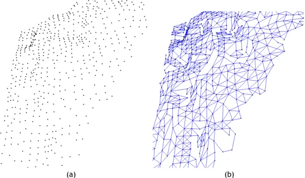
(a) (b) Figure 3.1: (a) Corrugated Cloud Point; (b) Corrugated Mesh.

Figure 3.2: Side view of a corrugated Mesh

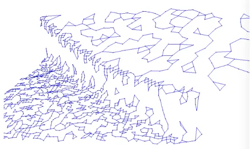
• Sharp feature that form Drifting. If the direction of a mesh changes it will forme a sharp feature, one example are mechanical objects, in those cases if the variance of direction is about 90º it doesn’t fold over itself, therefore, it is easy to calculate the proper mesh in a good density and uniform sample. However, when the sharp feature has 20º to 60º of curvature, its considered that it folds over itself, thus, making it impossible to determine a good orthogonal projection of its points to make further calculations, as shown in Figure 3.3.

In this cases, even with a good density sample, in the area where the mesh changes its direction, the points will not have their neighbours more close to the ones that it should connect, which are the ones in the edge of the change of direction. As shown in Figure 3.3, in blue are the two closest connection of each point, which in the area of the change of direction, this connections are almost all wrong from the desired ones.

• Abrupt variance of point density. When the point of a Cloud Points are not well dis-tributed, or well sampled, it may create that some areas of the mesh already formed, the

(36)

Figure 3.3: Mesh with abrupt changed of point density

next point that should be connected with the mesh, is too far. The designation of being too far, comes from the medium distances of each point from the already created mesh, so, if in any case the supposed next point to be connected is much higher then the medium distance it will be considered that the density changed drastically in this area of the mesh. Calculating this is impossible, because, there is no information about the supposed next point to be connected.

Figure 3.4: Abrupt variance of point density

The implication of the variation of density points is as shown in Figure 3.4, for each point in blue is represented its two closest other points (neighbours), which in the left side of the figure it start well sampled and the representativity of the pretended mesh is good, while in the middle and right side the density stops to be uniform, therefor, starting to create some separate zones of connections, instead of being uniformly connected.

(37)

3.4 Algorithm Overview

As aforementioned, this dissertation presents a new approach on the Simplicial surface methods. A skeleton-mesh is formed by a set of rules and procedures to each point of the Cloud Point and therefore a mesh-growing algorithm is applied using the connectivity information obtained previously by the skeleton-mesh. The algorithm presented in this dissertation is divided in two main section:

1. Skeleton Mesh 2. Triangulate the mesh

3.5 Skeleton mesh

This section describes how to get the topological and the points connectivity information from the Cloud Point. This information is obtained after the creation of a ring of connections around each point to its neighbours, while applying some rules to form those connections.

This connections create a skeleton mesh, which will not be the final stage of the final mesh, but instead it is used to guide the reconstruction of the object from the Cloud Point, given to the algorithm, the topological information needed to compute the final mesh.

To do this, some rules and processes are needed to adquire the skeleton mesh. So, the steps for this section are:

1. k-Nearest Neighbours. 2. Reduce Neighbours 3. Dominante Plane. 4. Create Star.

3.5.1 k Nearest Neighbors

This step will try to create for each point a ring of connections around it, hereupon, this kind of algorithm require the local information about the points and its surroundings. In other words, it is required that each points knows the information of its neighbourhood, i.e. which points belong to it.

To create the neighbourhood with size S of each point Pn, it is required to search those points,

which is the calculus of the S nearest points of each point Pn of the Cloud using the Euclidean

distance between them. It the most time consuming step, since the Cloud Point doesn’t have any kind of topologic information, it would be necessary to make a global search on the Cloud Point.

Let the search be O, then the cost is n.O(n) where n is the total points of the Cloud Point. For the point P = (px, py, pz)and let Q = (qx, qy, qz)another point of the cloud, the distance

(38)

d =

√

(px− qx)2+ (py− qy)2+ (pz− qz)2 (3.1)

To cut the expensiveness of this step, i.e. to avoid the global search, one adicional step is required. This new step is a pre-processing to the Cloud Point, which is needed to implement a local approach on the search of each points neighbour. To do this, one of the following algorithms can be used: octree, kd tree, clustering or bounding box. Any of this methods will reduce the search of each point drastically, by dividing the whole Cloud Point into smaller blocks.

The choose of any of this methods isn’t importante, since, in the end, after any of those methods are implemented, for each point will be saved only the (k = 30) thirty neighbours more close to them. This value is chosen based on experiments made on the course of the work.

For example, if it is chosen to use the octree method to calculate the local region, it is possible to reduce the complexity of the algorithm by n.O(n) to n.O(81) (on the ideal case, where each cube or node has three point, so, the sum of the cubes where there point n is located and each other adjacent cube make a total of 81 points, note that all cubes need to have the same size). In a real example, where the Cloud Point has 600.000 points, each search is reduced in 98,65%. Even if the k = 30 neighbours is not obtained by the cube located in n and its adjacent ones, one more level of adjacent cubes are added. In this cases the total search for each point can be higher then 81, but will always justify the use of it, because the gains are enormous to the use of global search. After this step, each point will now have in its structure a list of its k = 30 closest neighbours.

3.5.2 Reduce Neighbours

When creating a mesh from a Cloud Point, each point p needs to be connected to its neighbours

Qn ={q1, ..., qn}, so it could form edges and therefore triangles. If the point p is located on a

smooth part of the pretended mesh of the object that is formed by the points of the Cloud Point, it is straightforward to say that the Qnneighbours are the correct ones. Where the difficulty is

only the find the value of n, which in part is not difficult to find (This step is explained later). For example, point p and the neighbours Qn can be represented i.e. for five neighbours n = 6

(Q6 = {q1. . . q6}) that form a ring around the point p, that can be represented in 2D as an

hexagon. So when Q5is connected with Q1the hexagon is completed and the point p is set as

completed and no more neighbours are used. Hereupon, there are two factors that can influence the final result of the construction of the polygon, which are:

1. Point Density 2. Very sharp curves

3.5.2.1 Point Density

Continuing the example given in Reduce Neighbours 3.5.2, if a rule is set to require the point

(39)

Figure 3.5: Point Density (top view of the mesh)

to create a polygon around the point p. In this case, is required to expand the quantity of the neighbours to form the polygon. In short, the required number of neighbours to form a polygon around point p is unknown prior to trying to create one. It should be noted that if all neighbours are used to create the polygon, it could form a invalid one.

3.5.2.2 Very sharp curves

Figure 3.6: Very sharp curves (2D view of a side cut of the mesh)

If the mesh has very sharp curves, then it can be divided in two dominant planes. Near where the curve occurs, the points there have their closest neighbour points from each plane, while they should only connect to points from the plane where it belongs. And there can also be points that belong to each plane since those are points of intersection by both planes, making those to have neighbour of both planes (that are correct ones). So, since the point p of the curve, as shown in Figure 3.6, have its neighbourhood, Qn, on its belonging plane and the other near

plane, the five points Q = 5 are located in one direction from the point p, which is the direction where the curve is located on the 3D space as shown in Figure 3.6. With this in mind and also as shown in this Figure we can see that the example given in Point Density 3.5.2.1, i.e. will also fail to create a polygon around the point p, more specific, a pentagon. In this case, unlike in Point Density 3.5.2.1, even if the quantity of neighbours is increased it will fail, because it

(40)

connects to the different plane.

3.5.2.3 Leading Idea

The goal is to form a polygon around point p, with his neighbours Qn while the polygon to be

created will use the minimum neighbours and the closest ones to complete the polygon, it isn’t clear which type of polygon it will create. As it can be seen in Figure 3.5, to complete the polygon it is required to use Q = 8 neighbours, to create a non uniform octagon. It also requires that this kind of polygons, have all their points smoothly aligned, so that each edge had as closest just two others edges from it (the closest measure is by the angle they form). While this happens in Figure 3.6, it doesn’t happen in Figure 3.6.

The idea behind the step Reduce Neighbours 3.5.2 is to eliminate the not required neighbours while eliminating some noise. Since there are thirty neighbours from k-Nearest Neighbours 3.5.1, which make the neighbourhood of each point p with too much noisy information. There can’t be a straightforward elimination of the farthest neighbour, because sometimes, as ex-plained in Very sharp curves 3.5.2.2, the nearest neighbour can be the wrong one, and the farthest can be the correct.

So, in order to achieve the reduce of the size of the neighbourhood, eliminating the wrong and noisy neighbours, the next step is necessary. Beginning with the closest neighbour q1,the edge

that is formed with the point p can’t have the angle lower then 30º with another edge formed with the others neighbours qn.

The threshold on the angle, comes from the idea that each polygon has inconstante internal angles, while some angle are bigger then 90º others can have angles as low as 30º. The threshold value was defined by several tests and validation. Through that value the algorithm will always form a polygon.

(a) (b)

Figure 3.7: Sem a aplicação da regra (left); Ângulos maiores que 30º (right).

As shown in Figure 3.7, with less then eight edges it will form a polygon, more specific, now with five neighbours it will create 5 edges and therefor a pentagon. In this case is not where the algorithm takes the most from the rules described previously, on the other hand, as shown in Figure 3.8, it can be noted there that a lot of wrong neighbours got eliminated, i.e. lots of the connections to the points located in the wrong plane are now eliminated.

(41)

(a) (b)

Figure 3.8: Sem a aplicação da regra (left); Ângulos maiores que 30º (right).

that is wrong, so p will not make a smooth polygon with its neighbours. This problem will be solved in the next step.

3.5.3 Dominante Plane

As can be concluded by the previous step, there is still some bad connection between points and their neighbours on very sharp curves. In short, when trying to connect points with their closest neighbour, this connection could be topologically incorrect from the pretending mesh. Hereupon, there is required to calculate the local plane focused on the point p, so that the edges that deviate from it will be eliminated.

3.5.3.1 Tests

In the literature, the most used algorithm to determine the normal vector of a set o point that form a plane is the use of the Principal Component Analysis (PCA). The PCA involves a mathe-matical procedure that transforms a number of (possibly) correlated variables into a (smaller) number of uncorrelated variables called principal components. In computational terms the principal components are found by calculating the eigenvectors and eigenvalues of the data co-variance matrix. This process is equivalent to finding the axis system in which the co-co-variance matrix is diagonal. The eigenvector with the largest eigenvalue is the direction of greatest vari-ation, the one with the second largest eigenvalue is the (orthogonal) direction with the next highest variation and so on.

Let A be a n× n matrix. The eigenvalues of A are defined as the roots of:

determinant(A− λI) = |j(A − λI)| = 0 (3.2)

where I is the nxn identity matrix.

This equation is called the characteristic equation (or characteristic polynomial) and has n roots. Let λ be an eigenvalue of A. Then there exists a vector x such that:

(42)

Ax = x (3.3)

To find a numerical solution for x we need to set one of its elements to an arbitrary value, say 1, which gives us a set of simultaneous equations to solve for the other other elements. If there is no solution we repeat the process with another element. Ordinarily we normalise the final values so that x has length one, that is

x.xT = 1 (3.4)

In the case presented in this dissertation, it deals with 3D data which gives a (n x 3) matric of

x. which gives a 3 x 3 covariance matrix as′An×3× A3×ngives a matrix of size (3 x 3) A3×3.

So, a 3 x 3 matrix A with eigenvectors x1, x2, x3, and eigenvalues λ1, λ2, λ3 so:

x.xT = 1 (3.5)

Each eigenvalue corresponds to an eigenvector. In this dissertation the maximum eigenvalue is being used to find its corresponding eigenvector. This is a column vector which stores the (x,y,z) coordinates of the normal position. Normalising this vector will set it as a normal vector from the point used to create the covariance matrix.

Figure 3.9: Vector normal usando eigenvector a azul (left).

As shown in Figure 3.9, in blue is the normal vector obtained by the PCA, while the required normal vector for the intended dominante plane is at orange. Therefore a new way to determine the normal vector is used as explained in the next Section.

3.5.3.2 New method

It is clear that the eigenvector does not solve the problem presented before, so it is required to calculate the predominante plane which the point p is on. So, to do this, its gonna be calculated every possible plane with point p on it and the most appropriated plane is chosen between them.

(43)

There are three steps to make to find the plane, which are:

1. Find normal vectors 2. Group normal vectors

3. Choose of the normal vector & Clean

3.5.3.3 Find normal vectors

For each pair of edges that form a angle inferior to 160º between each other, the normal vector will be calculated. For example, for vectors ⃗u = −→q1pand ⃗v = −→q2p, if between them the angle θ (Eq. 3.6) is inferior to 160º, the vector ⃗n(Eq. 3.7) is calculated, which then is transformed to the normal vector (Eq. 3.8).

θ = arccos ( u· v ||u|| ||v|| ) (3.6) ⃗ n = u× v (3.7) ⃗ n = ( _n n· n ) (3.8)

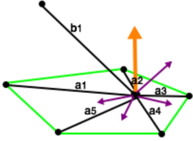
Choosing the angle 160º as threshold for calculating the normal vectors, makes that each edge will be used more then two times to generate a normal vector (normally it should generate just two normal vector, since each edge can only have two triangles, therefore, for each triangle one normal vector). This will help on the calculation of the dominate plane, because, the edges that really belong to the desired plane, have similar normal vectors and with this it will create a intensification on the determination of this normal vectors. While edges that doesn’t belong to he desired plane, will create normal vectors with quite different directions.

As shown in Figure 3.10, in green is the plane that is pretended to be calculated, in orange is the vector that represents the grouped normal vectors calculated by the edges a1. . . a5 and in

purple is the normal vectors calculated by the edges b1 with an. In other words, there exist

≈4 normal vectors (purple) with completely different directions and there is ≈8 normal vectors

(orange) with same identical directions.

3.5.3.4 Group normal vectors

As mentioned in the previous step, the normal vectors between each pair of edges with less then 160º can be grouped by their proximity from other normal vectors. So, for each of the normal vector, its set a counter, that will be incremented for each normal vector that has less than 10º with his. Furthermore, for each of those groups there will be calculated a new normal vector,

−−−−−→

(44)

Figure 3.10: Cálculo das normais

3.5.3.5 Choose of the normal vector & Clean

After all normal vectors −−−−−→nM ediahave been calculated from all possible sets of each point p, there is the possibility that two or more of this normal vectors have the counter of how many vector have been used to calculate them, with the same value. As this happens and to minimize the error in the choosing of the proper normal vector, a mean from this normal vectors that have the same counter value is made to the final−−−−−→nM edia.

At last, with the normal vector predominant calculated, there will be calculated the angle θ (Eq. 3.6) from this normal vector with the edges that exist in the point p and for each of this edges that doesn’t have a angle θ entre 75 < θ < 105, they will be deleted.

3.5.4 Create Ring

As referenced in Section 3.5.2 Reduce Neighbours, each point p has at maximum twelve con-nection (edges) with its neighbours. But as the aim is that each point p makes between a square and a octagon (4 to 8 connections), twelve connection goes far from the final aim. The ideia of using twelve connection was to help on detecting good connection in areas of very sharp curves. Because, even using the ideia described in Section 3.5.2.3 Leading Idea, where the connection on its neighbours is reduced, at same time trying to find the correct neighbours around the point p, in very sharp curves using only 8 neighbours might not be enough to find the correct neighbours around the point p, since they can still be in the same direction.

In areas with very sharp curves, the twelve neighbours connected to point p will be reduced as described in Section 3.5.3 Dominate Plane, where the connection that aren’t close to the dominante plane will be deleted, so reducing the size of the neighbourhood of point p. But as in areas where there isn’t any kind of curve, the point p will have a lot of noise neighbours, this is, around point p (360º), if the allowed is 30º between connections, this will make twelve connection at maximum. In real cases, this twelve connection are noisy connections, connecting to distant neighbours, as this neighbours are also near the dominant plane of the point p. To solve this, is just to reduce the neighbourhood of each point p to eight connection with the

(45)

closest neighbours.

3.5.4.1 Interconnection

In order to reduce further the noisy connections with neighbours, each of this connections from

pto qn, should have also a connection from qn to p, i.e. each connection must have a two

way connection. If this doesn’t happen, this connection will be deleted. This method is used since the probability of a connection to be correct increases when both point sees each other as connected neighbours.

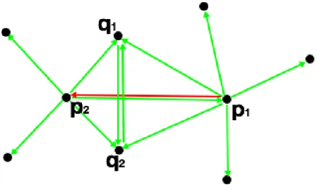
Figure 3.11: Descrição da Imagem

As seen in Figure 3.11, q1and q2, have between each other a connection of neighbour point, as

the p1and p2doesn’t. i.e. there is a connection from p2to p1while from p1to p2doesn’t exist,

so, as this connection isn’t two ways between them, it will be deleted.

3.5.4.2 Reducing the noise/error

In an attempt to further minimize noise and the error that exists between points p, for each point p it will be tried to reduce its neighbourhood to five, which could or not happen (it could stay at eight). To do this, for the sixth to the eighth more farthest neighbour, pq5. . . pq8, is

verified if the opposed connection, q5p . . . q8p, on their respective qn points, are the fourth or

more farthest connection. If this is true, this connection will be deleted. This reduces even more the connections made from each points p, but iff the elimination of this connections doesn’t reduce in excess the connection existing in qn.

3.6 Mesh Growing Algorithm

At this stage of the algorithm, the cloud point has already been topologically organized and with a skeleton mesh as been formed, made with connection from each point to its neighbours. Now,

(46)

the algorithm proceeds to the creation of triangles from the connections already formed, at the same time that some of them are deleted so that the mesh can be formed correctly.

3.6.1 Seed

To start triangulating the mesh, a point p must be chosen, as it will start the algorithm with it as the first point to be worked upon. The choice of this point takes into account the Section 3.5.3 Dominante Plane, where the point p that has the biggest number of correct connection, will be chosen. i.e. if he has the highest number of correct connection is because he happens to be on a area of the mesh that is flat, since the flat areas of the mesh are the ones with less incorrect connections and therefore making the choose of this point a good point to start.

3.6.2 Triangulation

For each point p that has connection that form edges a1...n = pq1...n, for each edge an it is

necessary to find other edge that has the lowest angle with an, so that this two can form a

triangle. So, for each an it will be calculated the angle between each other edges (minus the

edge that could already forming a triangle with an) and the one that makes the lowest angle

will be chosen to possibly form a triangle between them. The angle between this two edges cannot be ever higher then 100º.

For example, if a1= pq1and a2 = pq2 are chosen as edges with less angle between them, it is

required to verify if the edge oppose to the point p, i.e between q1 and q2, is already formed

or not. If the edge was already formed previously, so there are already the three edges needed to form the triangle between a1and a2. If this is not the case, it is required to create the edge

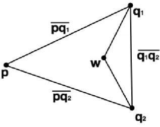
and its correspondent connections between q1and q2.

Figure 3.12: Attempt to create triangle q1pq2

At this point, there is still needed to verify if the triangle can be formed by q1 and q2, i.e for

the triangle formed to be valid, at q1and q2can’t be no other connection between q1p, q1q2and q2p, q2q1, respectively, as shown in Figure 3.12.

(47)

At this stage of the algorithm is necessary to force the creation of triangles, so that the expansion of the mesh doesn’t stop, i.e, if it does not force the creation of the triangle, the expansion of the mesh can stagnate in an eventuality that is stops in all points around the mesh already created.

As shown in Figure 3.12, the edges q1w and q2w will be eliminated, so that the triangle can

be formed. The point w, will be put in a list of point for post-processing, which will add this point to the mesh in the end. The same will not happen in Figure 3.13, since here there is only eliminated the edge q1wand where the point w continues valid in the mesh.

Figure 3.13: Attempt to create triangle q1pq2

3.6.3 Final

The final step is to add all points that formed a new triangle in the Section 3.6.2 to a list which will be queued to create new triangles. The algorithm will then execute for each point of this list, taken the point out of it and adding new points as new triangle are formed.

(48)

3.7 Experimental Results

The implemented reconstruction algorithm as been tested in a large real world data (Figure 3.14). This cloud point has 657.916 points, that where reproduced by a lazer scan of a person head. Since this is a complex object to apply a complete reconstruction algorithm we will apply a custom octree that will divide the object in sub objects with 5000 points. Then, we will work in each of the sub objects, which are then used to study and identify the difficulties of this type of algorithm. Some examples are represented in the following sections.

(49)

3.7.1 Corrugated and Ondular Plane

Figure 3.15: Pre-Mesh of a Sub-set of points from the Object

Figure 3.16: Triangulated Sub-set of point from the Object

3.7.2 Sharp Feature

The mesh folds over itself, creating a≈ 45º over its two sub-planes. As shown in Figure 3.18, the triangulated is not complete, this happens because the skeleton-mesh created to guide the mesh growing algorithm, detects that there are two sub-planes, therefor it doesn’t create

(50)

connections between points of the different planes. There must be also noted that from the two sub-planes the point density is different.

Figure 3.17: Pre-Mesh of a Sub-set of points from the Object

(51)

3.7.3 Sharp Feature with Variant Point Density

Figure 3.19: Skeleton mesh

Reconstructing triangulated surfaces from unorganized points through local skeletal stars

Engenharia