Source localization in a time-varying ocean waveguide
Cristiano Soaresa)
Faculdade de Cieˆncias e Tecnologia, Universidade do Algarve, Campus de Gambelas, 8000-Faro, Portugal Martin Sideriusb)
SACLANT Undersea Research Centre, Viale S. Bartolomeo 400, 19138 La Spiezia, Italy Se´rgio M. Jesusc)
Faculdade de Cieˆncias e Tecnologia, Universidade do Algarve, Campus de Gambelas, 8000-Faro, Portugal 共Received 4 September 2001; revised 15 July 2002; accepted 29 July 2002兲
One of the most stringent impairments in matched-field processing is the impact of missing or erroneous environmental information on the final source location estimate. This problem is known in the literature as model mismatch and is strongly frequency dependent. Another unavoidable factor that contributes to model mismatch is the natural time and spatial variability of the ocean waveguide. As a consequence, most of the experimental results obtained to date focus on short source-receiver ranges共usually ⬍5 km兲, stationary sources, reduced time windows and frequencies generally below 600 Hz. This paper shows that MFP source localization can be made robust to time–space environmental mismatch if the parameters responsible for the mismatch are clearly identified, properly modeled and 共time-兲adaptively estimated by a focalization procedure prior to MFP source localization. The data acquired during the ADVENT’99 sea trial at 2, 5, and 10 km source-receiver ranges and in two frequency bands, below and above 600 Hz, provided an excellent opportunity to test the proposed techniques. The results indicate that an adequate parametrization of the waveguide is effective up to 10 km range in both frequency bands achieving a precise localization during the whole recording of the 5 km track, and most of the 10 km track. It is shown that the increasing MFP dependence on erroneous environmental information in the higher frequency and at longer ranges can only be accounted for by including a time dependent modeling of the water column sound speed profile. © 2002 Acoustical Society of America.
关DOI: 10.1121/1.1508786兴
PACS numbers: 43.30.Wi, 43.60.Pt, 43.30.Pc关DLB兴
I. INTRODUCTION
Matched-field processing共MFP兲 is an inversion method that allows a source to be located from receptions on an array and has mostly been applied to sound sources in the ocean1,2
共see also Ref. 3 and references therein兲. The MFP technique
compares the received field with replica fields generated for all possible source locations using an acoustic propagation model. Localization results degrade when inaccurate or in-sufficient data is used as input to the propagation model. This is often called the model mismatch problem and can occur when environmental information, such as the ocean sound speed, is not known in sufficient detail. Mismatch also oc-curs when there is uncertainty in the measurement geometry, such as receiver array position.4,5In classical MFP the envi-ronment and measurement geometry are assumed known and the inversion search space includes only parameters relating to the source location.
To mitigate model mismatch, a class of matched-field processors, including the so-called uncertain processors
共OFUP兲6and the focalization processor,7emerged in the past
decade. These processors include both environmental and
geometric parameters in the search space, hence reducing potential model mismatch problems.关Throughout this paper geometric parameters are those related to source and receiver positions, as well as propagation channel dimensions 共e.g., water depth兲. Environmental parameters are those that char-acterize acoustic properties of the propagation channel共e.g., seabed sound speed兲.兴 It has been shown that these proces-sors can successfully locate acoustic sources in the ocean even if the environmental knowledge is limited.8 –10
Focalization and OFUP should perform well if the most important environmental and geometric parameters are in-cluded in the search space. This becomes more difficult as source frequency increases and therefore the relevant time and length scales needed to describe the environment de-crease. This is one reason why most experimental studies on both classical MFP and focalization have been applied to data at frequencies below 500 Hz. However, sound sources in the ocean often occur at frequencies above 500 Hz. The sources may be natural共e.g., from marine life兲 or man-made
共e.g., engines or sonar sound projectors兲. The main issue
be-ing addressed in this paper is to experimentally test whether MFP can be applied in a shallow water scenario at frequen-cies up to 1500 Hz. It will be shown that at these higher frequencies, the variability of the water column sound speed plays an important role that needs to be included in the pro-cessing.
The data considered here was collected in May, 1999
a兲Electronic mail: [email protected]
b兲Electronic mail: [email protected]; Current address:
Science Applications International Corporation, 10260 Campus Point Dr., San Diego, CA 92121.
during the ADVENT’99 sea trial. One of the goals of this experiment was to test the performance of field inversion methods in shallow water under controlled conditions. The signals emitted were multitones 共MT兲 and linear frequency modulated 共LFM兲 sweeps in the bands 200–700 Hz and 800–1600 Hz. A vertical array was deployed on three sepa-rate days at ranges of 2, 5, and 10 km from the source.
In Ref. 11, Siderius et al. performed MFP inversion 共fo-calization兲 on the ADVENT’99 low frequency data. The data from 2 and 10 km ranges were inverted for both the source location and seabed properties. Time- and range-independent water column sound speed profiles were used for each of the two tracks considered. Their results indicate that for the 2 km track a consistent high correlation between measured and modeled broadband data can be obtained and this resulted in reliable estimates for the source location and seabed proper-ties. Inversion of data taken at 10 km showed increased vari-ability in estimates for both source position and seabed prop-erties. The conclusion is that the environmental variability can destroy coherent processing and propagation prediction of acoustic data leading to erroneous estimates for source location and seabed properties. In the case of the ADVENT’99 data this was true for the low frequency data at 10 km source receiver separation.
This paper reports successful source localization results using the ADVENT’99 data taken at ranges of 2, 5, and 10 km and up to frequencies of 1500 Hz. This is achieved through a focalization process that accounts for the time and space variability of the environment共including ocean sound speed structure兲. The focalization search space is directed using a genetic algorithm共GA兲.12As a further demonstration of the utility and robustness of the method, localization was tested using data from short arrays 共subapertures from the ADVENT’99 vertical array兲. Successful application of MFP to short arrays with few sensors is important for practical applications since long, vertical arrays may not always be available. Results will be presented in Sec. III showing suc-cessful source localization in the 800–1600 Hz band at 5 km range using four sensors with a total vertical aperture of just 8 m. Vertical apertures of this size may be possible even from the droop of a horizontally towed array.
II. THE ADVENT’99 EXPERIMENT
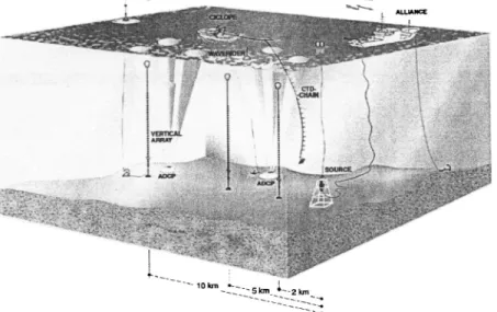
During the first three days of May of 1999 the ADVENT’99 experiments were conducted by the SACLANT Undersea Research Center and TNO–FEL on the Adventure Bank off the southwest coast of Sicily 共Italy兲. Figure 1 shows a drawing of the experimental setup. The bathymetry in the area has slight variations but the average water depth is 80 m. The acoustic sources were located at 76 m depth, mounted on steel framed tower that was sitting on the seabed. The signals were received on a 62 m-32 hydro-phone vertical array that was deployed at ranges of 2, 5, and 10 km. Only data from 31 hydrophones are considered in this paper共element 25 is missing兲. Broadband LFM and MT sig-nals were transmitted using two sound projectors, one for lower frequencies共200–700 Hz兲, and another for higher fre-quencies 共800–1600 Hz兲. The transmission time was around 5 hours for the 2 and 5 km tracks, and 18 hours for the 10 km track. The data used here has an estimated signal-to-noise ratio greater than 10 dB.
For sound speed measurements a 49-element conductivity-temperature-depth 共CTD兲 chain was towed by ITNS Ciclope. The CTD chain spanned around 80% of the water column reaching a maximum depth of 67 m, and was continuously towed between the acoustic source and the ver-tical array 共10 km track兲. The data was sampled every 2 s which corresponds to a vertical sound speed profile measure-ment approximately every 4 m in range. See Refs. 13 and 14 for a more detailed description of the experiment.
III. PARAMETER ESTIMATION USING GA AND SOURCE LOCALIZATION
The focalization procedure proposed by Collins et al.7 was adopted in this study to account for time-varying envi-ronments. This was accomplished using the following two-step algorithm:
共1兲 GA estimation of geometric and environmental
param-FIG. 1. ADVENT’99 sea trial setup with three vertical line array at positions 2, 5, and 10 km from a bottom mounted acoustic source. R/V Alliance is transmitting acoustic signals and collecting vertical line array data through an RF link. ITNS Ciclope is towing a CTD chain along the acoustic transmission track.
eters: in order to determine共focus兲 the array position and environment to be used in the source localization—step
共2兲.
共2兲 Exhaustive range-depth source localization with
param-eters obtained in step共1兲.
The matched-field localization problem usually does not include step 共1兲 since the geometric 共e.g., array position兲 environment 共e.g., sound speed profile兲 and bathymetry are assumed known. There is, however, always some uncertainty in these parameters and step 共1兲 is included here to accu-rately determine the optimal array position, effective bathymetry, and sound speed before application of the
step-共2兲 localization.
One of the difficulties associated with any MFP study is the choice of the environmental model used to represent the real environment where the acoustic signal propagates. Here, we define a baseline model that contains a mathematical de-scription of the real environment and constrains the attain-able set of solutions.
A. The baseline model
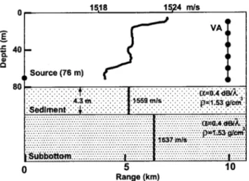
The baseline model consists of an ocean water column overlying a sediment layer and a bottom half-space, assumed to be range independent, as shown in Fig. 2. For step共1兲, the forward model parameters were divided into two subsets: geometric parameters and water column parameters. The geometric parameters include source range, source depth, re-ceiver depth, array tilt, and water depth. The parametrization of the water column will be explained later. The baseline sediment and bottom properties used for the experimental site were those estimated by Siderius et al.11 using the low frequency data set. Figure 2 shows an example of a sound speed profile measured close to the vertical array at 06:38 on May 2. This profile is typical of those measured during the experiment showing a double thermocline at 10 and 55 m depth with isovelocity layers in between.
B. The objective function
The focalization of the environment and geometry关step
共1兲兴 was posed as an optimization problem, that is, to find a
vector of parametersគ that maximizes an objective function. The objective function used here is the conventional fre-quency incoherent broadband processor, also called the Bar-tlett processor, and is defined as
P共គ 兲⫽1 Nn
兺
⫽1N
pគH共គ ,n兲CˆXX共n兲pគ共គ ,n兲. 共1兲
The factor CˆXX(n) is the sample cross-spectral matrix ob-tained from the observed acoustic field at frequencyn, N is the number of frequency bins, and pគ are the replica vectors to be matched with the data. All factors in 共1兲 have norm equal 1, hence the maximum attainable value of P(គ ) is 1.
The cross-spectral matrices were computed from the time series received on the 31 hydrophones using the lower frequency tones 共200 to 700 Hz with 100 Hz spacing兲 and higher frequency tones 共800, 900, 1000, 1200, 1400, 1500 Hz兲. Each ping of 10 s was divided into 0.5 s nonoverlapping segments, where the first and last segments were discarded, giving a total of 18 segments. Then, the 18 data segments were Fourier transformed, the bins corresponding to the mul-titone frequencies extracted, and the sample cross-spectral matrices computed. This procedure was repeated every 28 minutes for the 2 km track and at every 32 minutes for the 5 and 10 km tracks, for a total of 12 estimates for each track. Note that, for convenience and perceptibility, the ambiguity surfaces shown throughout this paper are only the odd num-bered surfaces out of the 12 estimates.
C. Model parameter estimation and source localization
To cope with the time variability of the acoustic field the source-receiver geometry and the environmental parameters were optimized using genetic algorithm 共GA兲 search. The GA settings were adjusted as follows: the number of itera-tions was set to 40 with three independent populaitera-tions of 100 individuals; crossover and mutation probabilities were set to 0.9 and 0.011, respectively. These GA settings were slightly re-adjusted as additional environmental parameters were in-cluded to the search space throughout this study.
The GA optimization was carried out using a varying number of environmental parameters depending on the track. Throughout this paper it will be explained which environ-mental and geometric parameters were included in each in-version, but only source localization results are reported. There is no intention of validating the environmental para-meters obtained throughout the various propagation tracks. The focalization step can produce a set of optimized para-meters that are not necessarily correct even with a match of the replica field with the array received field. In this case a so-called equivalent model is obtained.
Table I shows the geometric parameters of the forward model and their respective search bounds for each range track. Note that source and receiving array depth are coupled to water depth, and therefore they are referenced to the depth of the bottom and referred to as source and array height.
For each source range, GA optimization was first carried out for the lower frequency MT, where the sensitivity to model mismatch is expected to be lower. Then source local-FIG. 2. Baseline model for the ADVENT’99 experiment. All parameters are
range independent. The model assumes the same density and attenuation for sediment and sub-bottom.
ization ambiguity surfaces were generated for both frequency bands using replicas computed using the parameters esti-mated in the GA optimization. All replicas were computed using the SACLANTCEN normal mode propagation code C-SNAP.15
1. The 2 km track
Since model mismatch is less problematic at shorter ranges, the optimization关step 共1兲兴 for the 2 km track data set was performed directly on the higher frequency MT. The step-共1兲 parameter bounds for optimizing the array position are shown in Table I. The water column sound speed profile was linearly extrapolated down to the bottom using the two deepest sound speed values. No optimization was performed for the water depth since no significant water depth changes were expected in the relatively short range of 2 km.
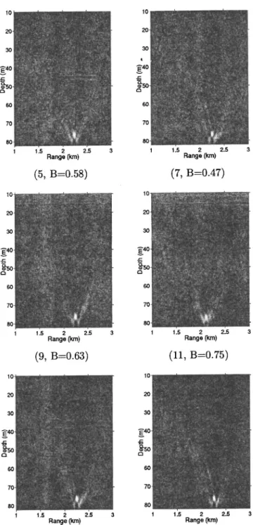
The step-共2兲 range-depth ambiguity surfaces were com-puted for source ranges varying from 1 to 3 km, and source depth between 10 and 80 m using the baseline environmental parameters and the previously GA estimated geometry. Figure 3 shows only the odd numbered ambiguity surfaces, and Table II summarizes the results obtained through time in terms of the mean and standard deviation. The time elapsed between surfaces is 28 minutes except between surfaces 2 and 3 共where transmissions were interrupted兲. All surfaces show a relatively stable ambiguity pattern with a clear peak standing out from the background at the correct source posi-tion. The standard deviation is low for the source parameters and the Bartlett power has mean of 0.57 共Table II兲. This relatively low Bartlett power can be explained by the large frequency band being used: in order to get the maximum average match, the model has to find a parameter set that yields the best overall matched-field response, but not the best single-frequency matched-field response. If the optimi-zation was carried out separately for each frequency, the op-timum parameter set would be different and a higher matched-field response would therefore be attained for each frequency. In Fig. 4 a comparison is shown between the rep-licas and the received field for the tones in the best and worst match case. The best match is generally obtained at 900 Hz
共0.77兲 and the worst match is obtained for 1500 Hz 共0.56兲.
A full optimization including all seafloor parameters has shown little dependence of the acoustic field in this fre-quency band. Moreover, fluctuations in the propagation
channel cannot be taken into account by inverting the seaf-loor. Therefore, for the remainder of this study seafloor prop-erties are not included in the search space.
2. The 5 km track
Having obtained stable localization results for the 2 km data set, the next step is to study the effect of a larger source-receiver range using the same procedure. First, the low fre-quency multitone data was processed in step共1兲 for the array position. Next, ambiguity surfaces were computed using the FIG. 3. Incoherent Bartlett ambiguity surfaces obtained for the 2 km track using six multitone frequency bins in the band 800 to 1500 Hz. B is the maximum Bartlett power obtained in each ambiguity surface.
TABLE I. Search bounds for the GA optimization of the geometric para-meters; source and height of the deepest receiver on the array are measured from the water-sediment interface and are therefore coupled with the water depth search parameter. Water depth was only searched for the 10 km track and held fixed to 80 m for the 2 and 5 km tracks.
Parameter
2 km 5 km 10 km
min max min max min max
Source range共km兲 1.8 2.6 4.7 5.8 10.0 11.0
Source height共m兲 1 10 1 10 1 10
Array height共m兲 1 15 1 15 1 15
Array tilt共rad兲 ⫺0.025 0.025 ⫺0.025 0.025 ⫺0.025 0.025 Water depth共m兲 80 80 80 80 78 82
optimized parameters and these are shown in Fig. 5. The figure shows a well resolved peak that correctly localizes the source in both range and depth.
Ambiguity surfaces were then computed for the higher frequency MT data set关after the step-共1兲 otimization of the geometry兴 and these are shown in Fig. 6. In this case the algorithm completely failed to localize the source. Close ob-servation of the surfaces reveals that in the first half of the run there is an ambiguity structure 共peaks and sidelobes of maximum correlation兲 close to the expected structure from the low frequency results共see Fig. 5兲, and also that surfaces
共4兲 and 共5兲 have the peak at the correct location. The
struc-ture that appears in surface共1兲 to 共6兲 disappears in surfaces
共7兲 to 共12兲 and this causes the true source location to be
completely missed. This result suggests mismatch in envi-ronmental model used in the second half of the run.
To help mitigate the environmental mismatch problem, the water column sound speed profile was also parametrized.
This increases the degrees of freedom of the environmental model and allows the step-共1兲 search to find an effective sound speed and adjust to the time varying acoustic recep-tions. The sound speed profile can be parametrized in several ways and combined with site measurements. To correct for possible depth errors 共and short-term fluctuations兲 in the towed CTD chain, a search over 4 m was included in the depth of the sound speed profile measurements used in the model. Another parameter included in the search space was the gradient of the sound speed profile in the portion between 67 m and the bottom, which is a region of the water column not covered by actual measurements. This is possibly very FIG. 4. Comparison of the predicted pressure with the measured pressure at
frequencies with best and worst match for each range. The single frequency Bartlett power is marked on each plot.
FIG. 5. Incoherent Bartlett ambiguity surfaces obtained for the 5 km track using six multitone frequency bins in the band 200 to 700 Hz. B is the maximum Bartlett power obtained on each ambiguity surface.
TABLE II. Summary of the source localization results for the 2, 5, and 10 km tracks in terms of the mean and standard deviation. The data used are the higher frequency MT共800–1500 Hz兲 transmissions.
Parameter
2 km 5 km 10 km
mean std mean std mean std Source range共km兲 2.23 0.041 5.44 0.048 10.6 0.24 Source depth共m兲 76.5 0.22 75.6 0.37 74.1 1.6 Bartlett power 0.57 0.072 0.60 0.047 0.37 0.057
important for predicting the acoustic field since the sound source was located near the bottom. For the 2 km track, the sound speed profile was completed by extrapolating the two deepest sound speed values down to the bottom. Including the gradient as a search parameter implicitly assumes that the sound speed behaves linearly as the depth increases but should provide a better description. Even if this is a simple and crude assumption, this parametrization was judged suf-ficient to model the last values of the sound speed close to the bottom. The third and last attempt to track the time vari-ability of the acoustic data in the 5 km high frequency data
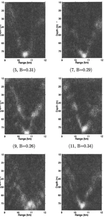
set was to include a full parametrization of the sound speed profile evolution through time using a set of data based em-pirical orthogonal functions 共EOFs兲. EOFs are basis functions9that can be obtained from a database and are very efficient to reduce the number of data points to be estimated. If historical data is available, an efficient parametrization in terms of EOFs should lead to a faster convergence and better resolution in the optimal solution since a large amount of information is already available and the search is started FIG. 6. Incoherent Bartlett ambiguity surfaces obtained for the 5 km track
using six multitone frequency bins in the band 800 to 1500 Hz. B is the
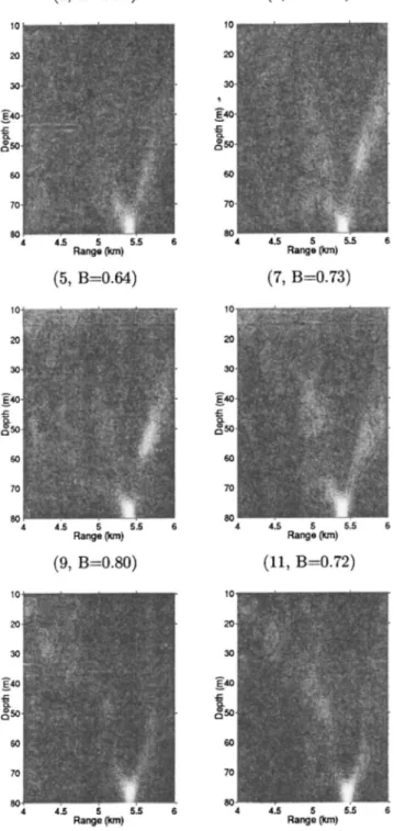
maximum Bartlett power obtained on each ambiguity surface. FIG. 7. Incoherent Bartlett ambiguity surfaces obtained for the 5 km track using six multitone frequency bins in the band 800 to 1500 Hz. The focal-ization step included estimation of the sound speed profiles via EOFs. B is the maximum Bartlett power obtained on each ambiguity surface.
closer to the solution. The EOFs are constructed from repre-sentative data by sampling the depth dependence of the ocean sound speed. To account for the variability of the sound speed, measurements taken over time and at different locations are considered. The EOFs can be obtained from a singular value decomposition of the sample covariance ma-trix C as
C⫽U⌳UH, 共2兲
where⌳⫽diag关1,...,N兴 is a diagonal matrix with the eigen-values n, U⫽关Uគ1,...,UគN兴 is a matrix with orthogonal
columns, which are used as the EOFs, H denotes conjugate transpose, and N is the number of data points in the water column. Using the sound speed measurements taken close to the vertical array, it was found that three EOF’s accounted for more than 80% of the water column energy. The modeled sound speed is written as
CគEOF⫽cគ¯⫹
兺
n⫽13
nUគn, 共3兲
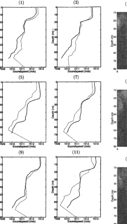
FIG. 8. Comparing sound speeds obtained by interpolation of real sound speeds with sound speeds estimated through EOFs using the higher
fre-quency MT共800 to 1500 Hz兲 at the 5 km track. FIG. 9. Incoherent Bartlett ambiguity surfaces obtained for the 10 km track using six multitone frequency bins in the band 200 to 700 Hz. The focal-ization step included estimation of the sound speed profiles via EOFs. B is the maximum Bartlett power obtained on each ambiguity surface.
where cគ¯ is the average sound speed profile. By trial and error, the search interval for the coefficients n combining the 共previously normalized兲 EOFs was chosen between ⫺5 and 5.
The total number of parameters included in the focaliza-tion step is now nine, four concerning the geometry, and five concerning the sound speed in the water column, correspond-ing to a search space with size 2⫻1015. Regarding the GA optimization and in order to cope with this larger search space, the number of iterations was set to 40, the number of individuals was set to 140, and the number of independent
populations was three which corresponds to about 1.5⫻104 forward models to be computed.
Observing the ambiguity surfaces obtained after accom-plishing the focalization step共Fig. 7兲, it can be seen that the main peak is always nearly at the correct location, within negligible variations, and the ambiguities are largely sup-pressed. In Table II it can be seen that the variability of the source parameters is of the same order of greatness as those obtained for the 2 km track and that the mean Bartlett power is even higher than that obtained for the 2 km track. Figure 8 shows plots comparing the sound speed profiles measured FIG. 10. Incoherent Bartlett ambiguity surfaces obtained for the 10 km track
using MT frequency bins in the band 800 to 1500 Hz. The focalization step included estimation of the sound speed profiles via EOFs. B is the maximum Bartlett power obtained on each ambiguity surface.
FIG. 11. Ambiguity surfaces obtained with the broadband conventional in-coherent processor for the 10 km track using the higher frequency LFM signals共820 to 1500 Hz兲, spaced by 23.4 Hz. B is the maximum Bartlett power obtained on each ambiguity surface.
close to the array and those obtained using the EOF expan-sion. In general it can be seen that there is a significant difference between the sound speed profiles being compared. There are at least two reasons to explain this difference: one is that the estimated profiles result from an integral of the sound speed profiles along the acoustic propagation path, and therefore include water column range dependency, if any, the other is that the estimated profiles result from a multi-parameter optimization procedure and therefore may accom-modate possible deviations of other environmental and/or geometric parameters, yielding the best matched-field re-sponse. An example is the sound speed profile gradient be-low 67 m共Fig. 8兲, that has often a nonphysical steep increase towards the bottom. In this paper there is no intention in validating the optimized sound speed profiles.
Finally, Fig. 4 shows that for this track the replica field at 900 Hz is well matched with the received acoustic field, and that the match at 1500 Hz is reasonable. The para-metrization chosen for the sound speed allowed therefore for modeling the environment such that localization results of high quality could be obtained for the high frequency data set.
3. The 10 km track
It was shown that the modeling scheme applied at 2 km failed to accurately localize the source at 5 km for the higher frequency data set. The strategy for environmental focaliza-tion followed for the 5 km track has shown to be effective for that track, i.e., the replica fields were successfully matched with the field received by the array. Now the question is whether the focusing method applied at 5 km works also at 10 km.
The optimization strategy was therefore repeated for the 10 km track data where the only difference is the temperature data set from which the EOFs are computed. Previously, since the sound speed profiles used were only those mea-sured close to the array, only time variability was taken into account. For this track to obtain the EOFs, a database of sound speed profiles was constructed with profiles updated every 5 minutes and comprising the whole 10 km track ac-quisition period. Note that, as the CTD chain was towed continuously between source and vertical array this database includes profiles that are both range and time dependent. As
previously, it was found that the first three EOFs were suffi-cient to represent the temperature field.
The focalization step included the geometric parameters of Table I and the sound speed profile parameters as ex-plained in Sec. II. The results obtained on the lower fre-quency data set are shown in Fig. 9 and indicate that the source location is well resolved over the whole time series, and the main peak is well above the background ambiguities. The source range was estimated with a mean value of 10.6 km with a small variation of approximately ⫾50 m, and a source depth estimate with a variation of about 3 m around the true value of 76 m. The Bartlett power over time is larger than 0.6, which means that the agreement between the model and the measured data is relatively good.
Then, the same two step procedure was applied to the higher frequency band data set. In order to reduce the mis-match possibly due to the higher frequency and the longer range, the water depth was also included in the focalization step in agreement with the search interval shown in Table I. The ambiguity surfaces obtained for the MT analyzed are shown in Fig. 10. It can be noticed that the main peak is not completely stable in its correct position, but it always ap-pears close to the correct location. The standard deviation is about 240 m in range and 1.6 m in depth 共Table II兲. This corresponds to an increase relative to the 5 km track, as expected, since over a higher distance the environmental variabilities are more significant. As it can be seen in Fig. 4, there are significant difficulties, in particular at 1500 Hz, where there is no match at all共Barlett power is 0.047兲.
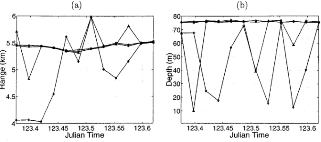
The source localization experimental results obtained for the MT are satisfactory with, however, a considerable in-crease of range and depth uncertainty with increasing range and with the high frequency data set. The issue is to know whether the modeling has reached its limitations, i.e., one can question whether the degree of sophistication of a range-independent environmental model is high enough to model this waveguide. For example, the hypothesis of a partially range-dependent model could be considered. Another hypo-thetical issue is whether it is possible to increase the amount of information inserted in the localization process by using more frequencies. Experimental results have shown that in-creasing the number of frequencies results in more consistent source localization estimates.9,10,16,17In order to test that pos-sibility, the LFM sweeps emitted in the same time slots as the FIG. 12. Source localization results over time for the 5 km track for differ-ent array apertures using the higher frequency MT 共800–1500 Hz兲: 共a兲 Range; 共b兲 depth. Each color stands for a different number of sensors: 31
MT were processed. A number of 30 frequencies ranging from 820 to 1500 Hz with a spacing of 23.4 Hz were se-lected. It can be seen that while for the tones a sustained variability in range is present, with the LFM signals it is possible to achieve periods of constancy共Fig. 11兲.
4. The effect of array aperture
After working with an array spanning around three quar-ters of the water column, and having obtained stable local-ization results at three different ranges, the goal now is to study the dependency of the MFP procedure on the array aperture. It is well known that, as the aperture is decreased less spatial discrimination is obtained, hence resulting in higher sidelobes relative to the main peak. In theory, even if the main peak-to-sidelobe ratio decreases with the array ap-erture, the main peak will always be at the correct position. However, in practice, with real data, geometric and environ-mental mismatch is always present and the acoustic field is observed during a limited time which creates a situation where a decrease of array aperture may indeed lead to a failure of source localization.
In the ADVENT’99 data set, reduced array aperture MFP was first applied to the higher frequency MT of the 5 km track, since for this range stable results with the full array were achieved, and could be used as reference. The array configuration used up to now had 31 elements spaced by 2 m. The procedure adopted to decrease the array aperture is to leave out sensors from the top and the bottom in such a way that the array is always centered in the water column, keep-ing the same spackeep-ing between sensors. The environment and geometry used were those obtained in the last focalization step for this range, hence exhaustive search is being carried out only for range and depth.
Figure 12 shows the results obtained by reducing the array aperture by successive factors of 2, i.e., from the full 31 sensors to 16, then 8 and finally to 4 sensors. The curve with circles shows the result obtained previously with the full aperture. Comparing the curves for range and depth ob-tained with half aperture 共asterisks兲 to those obtained with full aperture, only negligible difference is noticed. For eight sensors 共14 m of array aperture兲 it is still possible to obtain reasonable source localization results共curve with triangles兲, with, however, a larger spread in the estimates. The four
sensors case 共6 m aperture兲 represents a sampling of about 8% of the water column共curve with diamonds兲 where a sig-nificant degradation can be noticed.
Notice that the Bartlett power is highest for the four sensor configuration over the whole time even if the MFP procedure failed 共Fig. 13兲. The increment of the Bartlett power with the reduction of the array aperture is due to the reduced complexity of the acoustic field as seen by the array. The matched-field response is a measure of the similarity of the real acoustic field with the replicas produced by the nu-merical propagation model fed with different source loca-tions. If the aperture is small, then the uniqueness of the acoustic field along the portion of water column spanned by the field is lower, hence the match is higher.
Again, there is the possibility of compensating the lack of aperture by the addition of a large number of frequencies. Taking the LFM signals, a continuous set of frequencies is available, therefore 30 equally spaced frequencies between 820 and 1500 Hz were extracted and processed in the worst case situation of only four sensors. Figure 14 shows the im-provement obtained. There are still three outliers and some variability, but now it is possible to guess that 5.4 or 5.5 km might be the correct value for range and that the source depth might be between 70 and 80 m. This case shows that it was possible to partially compensate the lack of information ob-tained by reduced spatial sampling by increasing the number of frequencies and obtain a reasonable source localization at FIG. 13. Bartlett power over time for the 5 km track for different array apertures using the higher frequency MT共800–1500 Hz兲. Each color stands for a different number of sensors: 31共䊊兲; 16 共*兲; 8 共䉭兲; 4 共〫兲.
FIG. 14. Source localization results over time for an array aperture of 6 m using the higher frequency LFM sig-nals共820–1500 Hz, spaced every 23.4 Hz兲: 共a兲 range; 共b兲 depth.
5 km from a 6 m aperture vertical array with only four sen-sors共8% of the water column兲. Using the environmental pa-rameter set obtained during the focalization step with 31 hy-drophones strongly contributed for this result.
IV. CONCLUSION
Acoustic data were collected in a 80 m depth mildly range-dependent shallow water area of the Strait of Sicily, during the ADVENT’99 sea trial in May 1999. A vertical line array was deployed at three different ranges of 2, 5, and 10 km from an acoustic source. A series of multitone and linear frequency modulated sweeps were transmitted in two fre-quency bands of 200 to 700 Hz and 800 to 1500 Hz.
A two stage matched-field processing 共MFP兲 algorithm was applied throughout:共1兲 Focalization using genetic algo-rithms to search for the array position and environmental parameters giving the best fit between measured data and modeled replicas. 共2兲 Compute the MFP ambiguity surfaces in range and depth for source localization using previously determined array position and environmental characteriza-tion.
Concerning the analysis of the ADVENT’99 data, one of the conclusions in Ref. 11 is that the environmental variabil-ity at longer ranges can destroy coherent processing and propagation prediction of acoustic data. This paper com-pletes Ref. 11 with the following conclusions: 共1兲 As the source range and frequency are increased, the water column variability becomes more important and this needs to be ac-counted for in the modeling to obtain a good match between data and replica. 共2兲 The water column variability can be modeled using an EOF expansion and estimated with the focalization process.共3兲 With a full sound speed focalization precise MFP localizations could be obtained at all ranges and in both frequency bands共frequencies up to 1.5 kHz兲. 共4兲 The bottom parameters can be estimated from the short range 2 km track 共where variability and range dependence is less problematic兲 and held constant for all the other source-receiver ranges up to 10 km.
The attempt to decrease the array aperture showed that at 5 km source range, it was possible to achieve nearly cor-rect localizations with an array 4 times smaller than the ini-tial full aperture array, sampling only 16of the water column.
Using an increased number of frequencies allowed reducing the array aperture even further using only four sensors共121 of
the water column兲.
The results reported in this paper indicate that under controlled conditions and in a shallow water environment of low range dependence, it is possible to accurately model the acoustic field for ranges up to 10 km and frequencies up to 1.5 kHz to correctly localize an acoustic source over time if the optimized modeling process has taken into account pos-sible time variabilities in the water column. Moreover, these results indicate that the MFP technique can be made robust to model mismatch caused by the water column time depen-dence, if an adequate focalization procedure is incorporated,
even at high frequencies and ranges up to 10 km. This indi-cates that it may be feasible to carry out source localization at frequencies higher than typically considered for MFP even in the presence of strong environmental fluctuations such as internal tides, eddies, and fronts, if sufficient a priori infor-mation on the water column is available.
ACKNOWLEDGMENTS
The authors would like to thank SACLANTCEN for the support given during this study, in particular to Ju¨rgen Sell-schopp共the chief scientist of the ADVENT’99 cruise兲, Peter Nielsen and the NRV Alliance crew. This work was partially supported by PRAXIS XXI, FCT, Portugal, under the ATOMS project, Contract No. PDCTM/P/MAR/15296/1999.
1
H. P. Bucker, ‘‘Use of calculated sound fields and matched-field detection to locate sound source in shallow water,’’ J. Acoust. Soc. Am. 59, 368 – 373共1976兲.
2M. Hinich, ‘‘Maximum likelihood signal processing for a vertical array,’’
J. Acoust. Soc. Am. 54, 499–503共1973兲.
3A. B. Baggeroer, W. A. Kuperman, and P. N. Mikhalevsky, ‘‘An overview
of matched field methods in ocean acoustics,’’ IEEE J. Ocean. Eng. 18, 401– 424共1993兲.
4R. M. Hamson and R. M. Heitmeyer, ‘‘An analytical study of the effects
of environmental and system parameters on source localization in shallow water by matched-field processing of a vertical array,’’ J. Acoust. Soc. Am.
86, 1950–1959共1989兲.
5S. Jesus, ‘‘Normal-mode matching localization in shallow water:
environ-mental and system effects,’’ J. Acoust. Soc. Am. 90, 2034 –2041共1991兲.
6
A. M. Richardson and L. W. Nolte, ‘‘A posteriori probability source lo-calization in an uncertain sound speed deep ocean environment,’’ J. Acoust. Soc. Am. 89, 2280–2284共1991兲.
7M. D. Collins and W. A. Kuperman, ‘‘Focalization: Environmental
focus-ing and source localization,’’ J. Acoust. Soc. Am. 90, 1410–1422共1991兲.
8D. F. Gingras and P. Gerstoft, ‘‘Inversion for geometric parameters in
shallow water: Experimental results,’’ J. Acoust. Soc. Am. 97, 3589–3598 共1995兲.
9
P. Gerstoft and D. F. Gingras, ‘‘Parameter estimation using multi-frequency range-dependent acoustic data in shallow water,’’ J. Acoust. Soc. Am. 99, 2839–2850共1996兲.
10C. Soares, A. Waldhorst, and S. M. Jesus, ‘‘Matched-field processing:
environmental focusing and source tracking with application to the North Elba data set,’’ Oceans’99 MTS/IEEE Proceedings, Seattle, 1999, Vol. 3, pp. 1598 –1602.
11M. Siderius, P. Nielsen, J. Sellschopp, M. Snellen, and D. Simons,
‘‘Ex-perimental study of geo-acoustic inversion uncertainty due to ocean sound-speed fluctuations,’’ J. Acoust. Soc. Am. 110, 769–781共2001兲.
12
T. Fassbender, ‘‘Erweiterte Genetische Algorithmen zur globalen Optim-ierung multi-modaler Funktionen,’’ Ruhr-Universita¨t, Master thesis, Bo-chum, Germany, 1995.
13J. Sellschopp, M. Siderius, and P. Nielsen, ‘‘ADVENT’99, pre-processed
acoustic and environmental cruise data,’’ SACLANTCEN Undersea Re-search Center, Internal Report CD-35, La Spezia, Italy, 2000.
14M. Snellen, D. G. Simons, M. Siderius, J. Sellschopp, and P. L. Nielsen,
‘‘An evaluation of the accuracy of shallow water matched field inversion results,’’ J. Acoust. Soc. Am. 109, 514 –527共2001兲.
15
C. M. Ferla, M. B. Porter, and F. B. Jensen, ‘‘C-SNAP: Coupled SACLANTCEN normal mode propagation loss model,’’ SACLANTCEN Undersea Research Center, Memorandum SM-274, La Spezia, Italy, 1993.
16A. B. Baggeroer, W. A. Kuperman, and H. Schmidt, ‘‘Matched field
pro-cessing: Source localization in correlated noise as an optimum parameter estimation problem,’’ J. Acoust. Soc. Am. 83, 571–587共1988兲.
17S. Jesus, ‘‘Broadband matched-field processing of transient signals in