Use of GPU for time series analysis

(1)

Use of GPU for time series analysis

André Andrade Rodrigues

Versão Final Após Defesa

Dissertação para obtenção do Grau de Mestre em

Engenharia Informática

(2º ciclo de estudos)

Orientador: Prof. Doutor Rui Fernandes

Co-orientador: Doutor Machiel Bos

(2)

(3)

Dedication

This dissertation is dedicated to my parents. I would like to thank them for all their support in my academic and personal life.

(4)

(5)

Acknowledgments

This work could not have been done without the support of many crucial people, for that reason, I would like to express my innermost gratitude to my supervisors, Professor Rui Fernandes and Doctor Machiel Bos for all their support, patience and constant teachings.

I gratefully acknowledge the support of NVIDIA Corporation with the donation of the NVIDIA Quadro P6000 used for this research.

I would also like to thank all my friends at the Space & Earth Geodetic Analysis Laboratory (SEGAL) for all their support, making my working environment a pleasant one and for being more than just colleagues.

Last but not least, I would like to thank my girlfriend, family and friends for their encouragement and strong support.

(6)

(7)

Resumo

Os Sistemas de Navegação por Satélite, (do inglês Global Navigation Satellite System - GNSS) fornecem a posição de estações com uma precisão milimétrica. Estas posições não são con-stantes ao longo do tempo devido ao movimento das placas tectónicas nas quais as estações se encontram instaladas. O movimento das placas tectónicas não é igual em todas as partes do globo, o que leva à acumulação de stress em algumas áreas, aumentado assim a ocorrência de movimentos sísmicos. O conhecimento de tais movimentos é de extrema importância, bem como a determinação da sua incerteza.

O movimento tectónico é um processo muito lento e constante ao longo de milhares de anos. Como resultado, o movimento pode ser representado por uma tendência linear. Programas como o Hector podem estimar tendências lineares em séries temporais com ruído temporal correlacionado. Ruído correlacionado significa que as observações dos Sistemas de Navegação por Satélite feitas hoje são similares às dos dias anteriores, o que implica que haja menos informação do que se as observações fossem independentes. Esta é a razão pela qual a incerteza real do movimento tectónico estimado é entre 5 a 11 vezes maior do que quando esta correlação temporal não é considerada.

Infelizmente, ter em consideração essa correlação temporal na análise aumenta consideravel-mente o tempo de computação. Com o crescente número de estações GNSS e o aumento da duração das séries temporais existentes, é necessário acelerar essa computação. Este compor-tamento também pode ser encontrado em outras séries temporais geodésicas, como as do nível do mar observado em medidores de maré ou séries temporais da temperatura da superfície. Para estudos das alterações climáticas, é importante que, para além de estimar a elevação do nível do mar ou um aumento da temperatura, também as incertezas associadas sejam realísticas. O conjunto de software Hector foi desenvolvido com o objetivo de reduzir o tempo de com-putação tanto quanto possível. Nesta tese, investigaremos se o uso de uma potente Unidade de Processamento Gráfico (do inglês Graphics Processing Unit), vulgarmente conhecida como placa gráfica, pode reduzir ainda mais este tempo de computação. Até ao momento, nenhum software semelhante ao Hector usa placas gráficas para realizar o processamento de dados. Esta dissertação é, portanto, a primeira tentativa a ir nesse sentido.

Palavras-chave

CUDA, computação GPU, análise de séries temporais de sistemas de navegação por satélite, estimativa de tendência linear, estimativa de densidade espectral de potência.

(8)

(9)

Abstract

The Global Navigation Satellite System (GNSS) provides the position of stations with millimetre accuracy. These positions are not constant over time due to motion of the tectonic plates on which they are installed. The motion of tectonic plates is not the same all over the world, leading stress to build up in some areas, thus increasing the occurrence of earthquakes. The knowledge of such movements is of extreme importance, as is the determination of their un-certainty.

The tectonic motion is a very slow process that is constant over thousands of years. As a result, the motion can be represented by a linear trend. Programs such as Hector can estimate linear trends in time series with temporal correlated noise. Correlated noise means that GNSS obser-vations made today are similar to those of the days before, and it implies that one actually has less information than when all observations were independent. This is the reason why the real uncertainty of the estimated tectonic motion is between 5 to 11 times larger than when this temporal correlation was not considered.

Unfortunately, taking this temporal correlation into account in the analysis slows down the com-putations considerably. With the ever growing number of GNSS stations and the increasing length of the existing time series, it is necessary to speed up these computations. This behaviour can also be found in other geodetic time series such as sea level observed at tide gauges, and surface temperature time series. For climate change studies it is important that besides estimating sea level rise or an increase in temperature, also the associated uncertainties are realistic.

The Hector software package was developed with also the aim to reduce the computation time as much as possible. In this thesis we will investigate if the use of a powerful Graphics Processing Unit (GPU) can further reduce this computation time. So far, no Hector-like software uses GPUs to perform data processing. This dissertation is therefore the first attempt to go in that direction.

Keywords

CUDA, GPU computing, GNSS time series analysis, linear trend estimation, power spectral den-sity estimation.

(10)

(11)

List of Figures

1.1 Normal sequence of steps of using Hector to analyse a time series. . . 3

2.1 GPU computing applications. Source: CUDA Toolkit Documentation . . . 7

2.2 CUDA kernel hierarchy - Source: codingbyexample.com . . . . 8

2.3 CUDA kernel hierarchy IDs - Source: nvidia.com . . . . 9

3.1 Fourier Transform - Source: thefouriertransform.com . . . . 13

3.2 Fourier Transform summarised - Source: johndcook.com . . . . 14

3.3 Discrete Fourier Transform and its inverse - Source: wikipedia.org . . . . 14

3.4 Fourier Transform to Discrete Fourier Transform - Source: sp4comm.org . . . . . 14

3.5 Pinned Memory . . . 17

3.6 FFTW vs cuFFT & Laptop vs Server (Nvidia Quadro P6000) . . . 19

3.7 Nvidia Visual Profiler - estimatespectrum execution with a dataset of 10.000.000 entries . . . 22

3.8 Fourier Transform workflow on estimatespectrum program . . . 23

3.9 Power spectral density and fitted noise . . . 26

3.10 modelspectrum plot - KOSG station . . . 26

3.11 modelspectrum comparison for 20000 simulations - KOSG station, Kootwijk, Nether-lands Orange - laptop, Green - server . . . 28

4.1 CBLAS vs MAGMA & Laptop vs Server (NVIDIA Quadro P6000) . . . 35

4.2 Toeplitz Matrix. Source:wikipedia.org/wiki/Toeplitz_matrix . . . 36

4.3 estimatetrend - time distribution of an execution . . . 39

4.4 daxpy hierarchy calls . . . . 40

4.5 Time execution evolution for different sizes . . . 41

4.6 Logarithmic Scale - Time execution evolution for different sizes . . . 42

4.7 Sea level observed at Aberdeen, United Kingdom (blue dots). These observations have already been corrected for the effect of tides. Estimated trend plus seasonal signal is shown by red line. The black crosses are outliers. . . 44

4.8 Aberdeen station - Time execution evolution for different sizes . . . 45

4.9 Aberdeen station - Logarithmic Scale - Time execution evolution for different sizes 45 4.10 Aberdeen station - NVIDIA Quadro P6000 vs mid-range GPU . . . 46

(14)

(15)

List of Tables

1.1 Comparison between the GPUs used - Sources: nvidia.com and techpowerup.com 4

3.1 Computers Specifications . . . 17

3.2 FFTW vs cuFFT benchmarking on laptop . . . 18

3.3 FFTW vs cuFFT benchmarking on server . . . 18

3.4 estimatespectrum benchmarks . . . 24

3.5 modelspectrum benchmarks . . . 27

4.1 Computers Specifications . . . 33

4.2 CBLAS vs MAGMA - simple benchmarking - ordinary laptop . . . 34

4.3 CBLAS vs MAGMA - simple benchmarking - Server (Nvidia P6000) . . . 34

4.4 estimatetrend benchmarks . . . 37

4.5 estimatetrend benchmarks with Quadro P6000 . . . 38

4.6 Benchmarking of AmmarGrag step1 with Nvidia P6000 GPU . . . 41

4.7 Magma vs CUDA Kernel . . . 43

4.8 Aberdeen station benchmark . . . 44

(16)

(17)

Acronyms

API Application Programming Interface

BFKH Budapest Főváros Kormányhivatala

BLAS Basic Linear Algebra Subprograms

CPU Central Processing Unit

CUDA Compute Unified Device Architecture

DFT Discrete Fourier Transform

DSP Digital Signal Processor

EPOS European Plate Observing System

FFT Fast Fourier Transform

FFTW Fastest Fourier Transform in the West

FPGA Field Programmable Gate Array

GNSS Global Navigation Satellite System

GPU Graphics Processing Unit

I/O Input/Output

LAPACK Linear Algebra PACKage

MAGMA Matrix Algebra on GPU and Multicore Architectures

NVVP NVIDIA Visual Profiler

RAM Random Access Memory

SEGAL Space & Earth Geodetic Analysis Laboratory

UBI Universidade da Beira Interior

USAGE4TEA Updated Statistical Analysis of GNSS time-series Estimates for Tectonic

(18)

(19)

Chapter 1

Introduction

From the beginning of this century, the number of permanent GNSS stations worldwide has been increasing at a remarkably high pace to the point where, nowadays, there are several thousands of them. Due to various geophysical signals, in particular tectonic plate motion, these stations are constantly changing their position on the Earth’s surface. This motion is not the same all over the world, which induces the increase of stress in the Earth’s crust in the plate boundaries. The accumulation of stress increases significantly the likelihood of the occurrence of earthquakes. Consequently, in the past years, the creation of strain rate maps to gain insight into the stress accumulation became a subject of major importance for the geosciences and much development has been seen.

It is essential to accurately estimate the associated uncertainties to properly evaluate the com-puted tectonic motion and the derived strain rate maps. To do so, it is necessary to take into consideration that GNSS observations are correlated in time and space.

Some GNSS time series analysis methods consider only the temporal correlation within the time series. Hector is one of these software. Others consider only the spatial correlation that exists between the time series of different GNSS stations. Analysing temporal correlation is an ex-ceedingly slow process that requires a large number of computational resources, and this is the reason of this dissertation: to make Hector faster through the usage of GPU resources. Besdies GNSS time series this will also benefit the analysis of other geodetic time series such as those observed at tide gauges.

1.1 Objectives

The analysis of time series is a slow process. In the scope of European Plate Observing System (EPOS) [1], where SEGAL is a partner, there are presently around 700 stations with 10 years of data on average. To analyse the data collected by them, it is needed a whole day, which leads to an urgent need of making Hector faster, particularly because the number of stations to be routinely analysed are expected to increase significantly in the near future.

Hector is currently one of the best software available in the world for GNSS time series analysis, which is being used by numerous research centres all over the world.

Recently, SEGAL obtained a powerful NVIDIA GPU. The goal of this study is to adapt the source C++ code of Hector software to make it faster by using GPU capabilities and analyse its results on a normal GPU card and on a powerful one dedicated for scientific usage.

Hector is a software parallelised and already optimised to take advantage of CPU capabilities. However, analysing the daily position time series for few years may need some hours, even with software well designed and being constantly optimized as Hector. Williams [2] noted that the computation time for analysing 10 years of data was around 6 hours. This was in 2003, nowadays, computation capabilities have increased significantly. Nevertheless, we still need several hours to analyse 10 years of data of a network with 100 stations in a normal computer.

(20)

We will shown here the results of the usage of Hector software combined with GPU computation and evaluate the difference from a CPU-only usage.

1.2 Hector Software

Hector [3] is a software package written in C++ language that can be used to estimate the linear trend in time series with temporal correlated noise. Trend estimation is a common task in geophysical research where one is interested in phenomena such as the increase in temperature, sea level and position over time. It is well known that in most geophysical time series the noise is correlated in time and this has a significant influence on the accuracy by which the linear trend can be estimated [4] [5].

1.2.1 Hector Programs Bundle

Hector is a software package that comes with seven programs, described below: • estimatetrend - Main program to estimate the linear trend.

• estimatespectrum - Program to estimate the power spectral density from the data or residuals using the Welch periodogram method.

• modelspectrum - Given a noise model and values of the noise parameters, this program computes the associated power spectral density for given frequency range.

• removeoutliers - Program to find offsets and to remove outliers from the data.

• findoffset - Program to find the epoch of a possible offset in the time series.

• simulatenoise - Program to create files with synthetic coloured noise.

• date2mjd - Small program to convert calendar date into Modified Julian Date.

• mjd2date - The inverse of date2mjd.

The normal sequence of steps of the analysis of a time series using Hector are shown in Fig. 1.1. Since temporal correlation is taken into account, the first step is to select a model of this temporal correlation which is the same as choosing a noise model. The next step is to remove the outliers that may exist in the data. Afterwards the linear trend is estimated using the program ’estimatetrend’ which is normally the slowest program of them all. This program also estimates the noise parameters which can be used to predict the theoretical power spectrum of the noise. This is compared with the actual power spectrum of the observations. If they agree, then this confirms the choice of noise model was correct. If not, then another noise model needs to be selected and the steps need to be repeated.

(21)

Figure 1.1: Normal sequence of steps of using Hector to analyse a time series.

1.2.2 Hector Main Features

Hector main features include:

• Correctly deals with missing data. No interpolation or zero padding of the data nor an approximation of the covariance matrix is required (as long the noise is, or has been made, stationary [6]).

• Allows yearly, half-yearly and other periodic signals to be included in the estimation pro-cess of the linear trend.

• Allows the option to estimate offsets at given time epochs.

• Includes power-law noise [7], ARFIMA [8], Generalized Gauss-Markov [9] and white noise [10] models. Any combination of these models can be made.

• Allows taking the first difference of the data if power-law noise model is chosen (including combination of white, flicker and random walk).

• Comes with programs to remove outliers and to make power spectral density plots. • Provides a program + script to automatically detect offsets.

1.2.3 Hector License

Hector is free software. Its license is under the terms of the GNU General Public License as published by the Free Software Foundation.

(22)

1.2.4 Synthetic time series Generation - simulatenoise

simulatenoise is a program to generate time series with synthetic coloured noise. The

gener-ation procedure is based on the method described by Kasdin [11] where an impulse response, different for each noise model, is convoluted with a white noise time series resulting in the de-sired synthetic noise time series. Usually the convolution is performed using FFT (Fast Fourier Transform).

Throughout this document, benchmarkings using time series as input will be presented. To fa-cilitate the control over the size of these time series, it was used simulatenoise program to gen-erate them. Every benchmarking in this dissertation uses time series created by simulatenoise, except those where it is mentioned that real data were used.

1.3 NVIDIA Quadro P6000

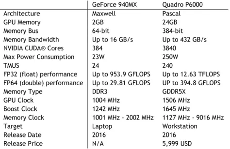
Recently SEGAL acquired a powerful NVIDIA GPU: Quadreo P600. The NVIDIA Quadro P6000 is a GPU oriented to science and virtual reality, and by the time it was released, in October 2016, it was, according to NVIDIA, the world’s most advanced professional graphics solution ever created. The next table helps to understand better the power of Quadro P6000 by comparing it against GeForce 940MX, a mid-range laptop GPU. Both GPUs are used in the benchmarks in the course of this dissertation.

GeForce 940MX Quadro P6000 Architecture Maxwell Pascal GPU Memory 2GB 24GB Memory Bus 64-bit 384-bit Memory Bandwidth Up to 16 GB/s Up to 432 GB/s NVIDIA CUDA® Cores 384 3840

Max Power Consumption 23W 250W

TMUS 24 240

FP32 (float) performance Up to 953.9 GFLOPS Up to 12.63 TFLOPS FP64 (double) performance Up to 29.81 GFLOPS UP to 394.8 GFLOPS Memory Type DDR3 GDDR5X

GPU Clock 1004 MHz 1506 MHz Boost Clock 1242 MHz 1645 MHz

Memory Clock 1001 MHz - 2002 MHz 1127 MHz - 9016 MHz Target Laptop Workstation

Release Date 2016 2016 Release Price N/A 5,999 USD

Table 1.1: Comparison between the GPUs used - Sources: nvidia.com and techpowerup.com

As can be seen from the table, Quadro GPU has totally disparate values from GEFORCE 940MX. The price of GEFORCE 940MX is not available as it is a mobile GPU, sold only directly to computer manufacturers, however, to comprehend the GPU target, it is available in laptops with a starting price of approximately 500€.

(23)

Chapter 2

State of the Art

In this chapter, concepts of CPU and GPU computation, CUDA programming and GNSS time series analysis will be presented.

This chapter begins with the history of the CPUs, from the first to the most modern ones, and from single to multi-core. Then there is an introduction to GPU computing, followed by its applications. After, CUDA programming will be explained and demonstrated with a code sample and will be introduced the CUDA concurrent, OpenCL. This chapter ends with an overview of GNSS time series analysis software.

2.1 CPU

The first commercial microprocessor, Intel 4004, was released by Intel in late 1971. It was a 4-bit processor with a maximum clock speed of 740kHz. A year later, Intel releases a new processor, the 8008. Intel 8008 was the first 8-bit processor, however, it was slower than the 4004 predecessor. In 1974 arises the Intel 8080 that increases the clock speed to 2MHz and separates the address and data bus. This processor was the basis for the Intel 8086, 16-bit processor that came up in 1978 and which is the ancestor of the commercial processors in use nowadays, the x86 family that includes processors such as Pentium and Core i7.

The following years continued to bring innovation to the processor industry, and other brands, such as Sun Microsystems or AMD, came into the market. This last one starts to face Intel with the Am386, a 32-bit processor with 40MHz of clock speed. But, was in early 1993 that the great innovation arises, the iconic Intel Pentium, with 66MHz of clock speed, 3.1 million transistors and 32-bit, this was the most advanced processor manufactured at the time. The Pentium family of successors kept leading the market until the 21 century and creased Intel as the main processor manufacturer company.

Nowadays, there are a lot of processors in the marker, although, Intel keeps leading, with the Intel Core family being the best sellers of the moment.

2.1.1 Evolution of CPU - From Single to Multi-core

CPUs began being single core devices. It implies that they could do only one task at once. With the constant evolution of computing and its needs, processors needed to enhance is capabilities, starting from being able to switch between tasks more quickly until the advent of the hyper-threading, introduced by Intel in 2002 on their Pentium 4 HT.

Hyper-threading debuted as a revolutionary approach to improve single-core CPU’s perfor-mance. Using hyper-threading, one CPU appears as two CPU’s to the operating system. Pre-tending that has more cores than really has, CPU uses its own logic to speed up his processing capabilities allowing the two logical cores to share physical resources [12]. For instance, the two virtual processors can borrow resources to each other when needed.

Hyper-threading, even though that is not as fast as two physical cores, can effectively increase CPU’s performance up to 30%.

(24)

Presently, single-core CPU’s are almost not in use. Low and middle-range CPU’s, including the advanced Intel Core i7 at its entry-level, commonly come equipped with 4 cores, that are actually two physical cores who act as 4 logical cores. Hyper-threading, although it is not a recent technology, is far from obsolete and it will certainly remain in use for much longer, due to its high efficiency that permits cost and size savings on processors. Every Intel processor comes equipped with hyper-threading, other brands have similar technologies.

Intel released recently the Intel Core i9-7980XE processor, equipped with up to 18 physical cores, which with hyper-threading, have 36 logical cores. Although, AMD has already the AMD Ryzen Threadripper 2990WX, with 32 physical cores which corresponds to 64 logical cores. The performance of both is still similar, as is their price [13].

2.2 GPU Computing

GPU computing is the use of a graphics processing unit (GPU) to accelerate applications running on the central processing unit (CPU) by processing some of the most intensive and consuming portions of the code.

GPU’s are specialised microprocessors optimised to do specific tasks. It runs at lower clock speed than CPUs but whereas a typical CPU consists of one to eight cores, a GPU consists of hundreds of smaller cores that operate together to process more data and in a faster way. A CPU can do any type of calculation, GPUs do more specific tasks.

The primary difference in the operating procedure of CPUs and GPUs is that considering a pipeline of tasks, CPU would take the first element of the pipeline and process the first stage, then the next, consecutively until the last, dividing the pipeline in time and applying all the resources in each stage. A GPU would instead divide the pipeline in space and not in time, dividing the resources among the different stages.

Essentially, the main difference between a CPU and a GPU is that the first is more appropriate for sequential and generic tasks, while GPU is better suited for particular tasks that can profit from parallelism.

2.2.1 GPU Applications

GPUs were firstly created in order to deal with 3D graphics and video. This is still nowadays the main use of the GPUs. More recently, with the advent of the cryptocurrencies, GPUs took a central role in mining the virtual currency.

GPU capabilities soon revealed interest from many other areas than just video rendering. Scien-tists immediately commenced to take advantage of GPU high processing capabilities, and these days, GPUs play an important role in scientific research. Data mining, deep learning, medicine, forecasting, mathematics, etc, are some of the areas that do not discard the usage of GPUs.

2.2.2 CUDA

Compute Unified Device Architecture (CUDA) [14] is a parallel computer architecture and pro-gramming model developed by NVIDIA, which introduced CUDA in 2006 and it is currently on its 10.1 version. CUDA includes a Runtime Application Programming Interface (API) and a Driver API. The differences between the two APIs are mainly that the Driver API is a lower-level API that can take control over the hardware and the Runtime API is a high-level API that allows the

(25)

developers to create programs with simpler code and without having a deep knowledge of the CUDA complexity and syntax.

CUDA has been achieving popularity mainly among scientists because it changed the paradigm of the parallel programming. Before CUDA or OpenCL, developers needed to understand the programming design of computer graphics processing to be able to create programs in other fields. Now, it can be done in a much simpler way, using CUDA.

CUDA also lets the programmers focus on the algorithm and abstract from the mechanics of par-allel programming. CUDA’s popularity led developers to create new libraries for GPU computing using CUDA or adapting existing libraries for CPU programming. This is also responsible for the increasing usage of CUDA amongst scientists, once it allows a faster and easier way to develop efficient parallel computing programs.

CUDA programs are usually written in C language, however, many other languages, application programming interfaces, or directives-based approaches are supported. Figure 2.1 synthesises valuable information to get started with CUDA, the main libraries available for the platform, all the programming languages supported and the NVIDIA devices enabled for CUDA as well their architecture and the minimum corresponding CUDA driver version. CUDA architectures have different constructions due to different goals or due to shifts in technology, this project uses two NVIDIA devices, one with Maxwell architecture and the other with Pascal, Maxwell’s successor. They have some variances with Pascal presenting higher bandwidth memory, unified memory, and NVLink as main differences to the previous architecture model.

In this dissertation is used C++ language and the libraries cuFFT and MAGMA. As CUDA is developed by NVIDIA, it can only be used in Nvidia GPU’s.

Figure 2.1: GPU computing applications. Source: CUDA Toolkit Documentation

2.2.3 CUDA Kernel

CUDA programming model is designed to process in parallel large amounts of data. The way to developing CUDA applications consists on the host device, the CPU, invoking special C functions (Kernels) that are executed N times by an array of threads that run the same code, however, each kernel has an ID and many threads execute each kernel in parallel.

(26)

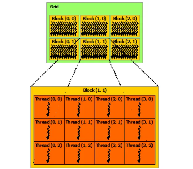
To better understand how a kernel works, one can look at figure 2.2. A CUDA program launches the already mentioned “special function”, i.e. a Kernel. In fact, to take advantage of CUDA parallel computing is not launched one Kernel, but a bunch of Kernels, which in turn, are ex-ecuted by another bunch of Threads. These Threads can be one, two or three-dimensional, (vector, matrix or volume) and they constitute a Thread Block. There is a size limit for Threads per Block, which in modern GPUs is 1024. Such as Threads, a group of Blocks can also be one, two or three-dimensional and it is called a Grid. The number of Grids depends on the size of the data being processed as well as the number of processors in the system [15].

Figure 2.2: CUDA kernel hierarchy - Source: codingbyexample.com

Each Thread, Block and Grid have their own ID 2.3. A Thread ID i is given by i = blockIdx.x +

blockDim.x + threadIdx.x where blockIdx.x is the x dimension Block identifier, blockDim.x is the x dimension of the Block dimension and threadIdx.x is the x dimension of the Thread identifier. i values will range from 0 to 1023.

(27)

Figure 2.3: CUDA kernel hierarchy IDs - Source: nvidia.com

2.2.4 CUDA Kernel Sample

Below is presented a very basic CUDA code. This can be called the CUDA Hello World, two arrays are summed in parallel and their result is stored on a third array. A normal CPU approach to this code would be to loop through the arrays sequentially and sum each position, in CUDA, it can be done simultaneously with each Thread performing one sum [16].

cuFFT sample

# define N 10000

// CUDA kernel

__global__ void add(int *da , int *db , int *dc) {

int i = blockIdx .x;

if (i<N) {

dc[i] = da[i] + db[i]; }

}

(28)

int a[N], b[N], c[N]; // Allocates memory on GPU

int *da , *db , *dc;

cudaMalloc ((void **)&da , N*sizeof(int)); cudaMalloc ((void **)&db , N*sizeof(int)); cudaMalloc ((void **)&dc , N*sizeof(int)); // Fills arrays with dummy data

for (int i = 0; i<N; ++i) { a[i] = i;

b[i] = i; }

// Copies input array from CPU to GPU

cudaMemcpy (da , a, N*sizeof(int), cudaMemcpyHostToDevice ); cudaMemcpy (db , b, N*sizeof(int), cudaMemcpyHostToDevice ); // Launches kernel

// Since there are N elements to process , and 1024 threads per // block , one just needs to calculate the number of blocks to get // at least N threads . Commonly , one simply divides N by the block // size ( being careful to round up in case N is not a multiple of // blockSize ).

int blockSize = 1024;

int numBlocks = (N + blockSize - 1) / blockSize ; // numBlocks -> number of threads blocks in a grid // blockSize -> number of threads in a thread block add <<<numBlocks , blockSize >>>(da , db , dc );

// Copies output array from GPU to CPU

cudaMemcpy (c, dc , N*sizeof(int), cudaMemcpyDeviceToHost );

// Free up the arrays on the GPU cudaFree (da ); cudaFree (db ); cudaFree (dc ); return 0; }

2.2.5 OpenCL

Open Computing Language (OpenCL) is a low-level API for heterogeneous computing. With the same programming model as CUDA, the two APIs have a quite similar purpose, although, there

(29)

are some differences between them. OpenCL is open-source and heterogeneous, and therefore, it means that OpenCL can run not only in GPUs but also in CPUs, Digital Signal Processor (DSP), Field Programmable Gate Array (FPGA) and other processor types.

OpenCL applications are portable, however, the performance is not. OpenCL needs kernels its to be compiled and when they are used in hardware for which they are not tuned, the performance decreases. Peng Du at al. (2012) [17] considers that with the lack of an automatic performance tuning for OpenCL applications, OpenCL cannot be established in the area of high-performance scientific computing.

[18] compared OpenCL against CUDA and for the conducted tests, the performance was just slightly different, with CUDA still prevailing the best. OpenCL is not as used and popular as CUDA, due to the market share totally subdued by NVIDIA [19], CUDA has a competitive edge over OpenCL. It is also pertinent to consider the wide variety of APIs available for CUDA that also contribute to making it the most dominant platform.

The advantage of OpenCL, considering the GPUs sector only, is the convenience of OpenCL on running in both NVIDIA and AMD GPUs.

2.3 GNSS time series Analysis Software

Hector is not alone in the world of GNSS time series analysis software. There are two other software that does the same as Hector: est_noise [20] and the first and perhaps the most popular CATS [21].

Hector is, however, the most advanced software available for GNSS time series analysis. Hec-tor differs from all the others due to two facHec-tors: HecHec-tor accepts only stationary noise, with constant noise properties and, most importantly, the way of creating Full Covariance Matrices. While others use Maximum Likelihood Estimation to create Full Covariance Matrices, Hector uses the Levinson–Durbin recursion algorithm implemented by Ammar and Grag and that is explained in detail in [3].

Maximum Likelihood Estimation requires O(n3₎_{operations for n observations, Hector reduces the}

number of operations to O(n2_{). Maximum Likelihood Estimation is a method that to invert}

ma-trices needs to go through all the matrix, so almost a brute-force method, while Levinson–Durbin recursion, the chosen method for Hector, uses a Toeplitz Matrix and Cholesky decomposition, which speeds up the process.

Once this project attempts to use Hector alongside GPU computation, is relevant to mention that so far, there is no GNSS time series analysis software that uses GPU cards, being this project the first attempting to accelerate the slow process of GNSS time series analysis.

2.4 Summary

An overview of the current state of GPU programming and its APIs, as well as the GNSS time series analysis software, has been provided in this chapter.

This chapter is essential to understand the following chapters, where one needs to have funda-mental concepts of GPU programming, CUDA, and Hector software.

(30)

(31)

Chapter 3

Fourier Transform

The best known of the Transforms, the Fourier Transform is the basis of this chapter and crucial for many parts in the Hector software. This chapter discusses the first efforts to turn Hector into a hybrid program that uses both CPU and GPU in its implementation. The chapter starts by explaining the Fourier Transform and the best libraries to execute on a computer the Dis-crete Fourier Transform. Then, it is provided a benchmark of Fast Fourier Transform using CPU and GPU libraries as well as the algorithms used by these libraries. Further, in this chapter, are shown the results of the transformation of two Hector programs, estimatespectrum and modelspectrum, that are programs totally dependent on FFTs.

3.1 Fourier Transform

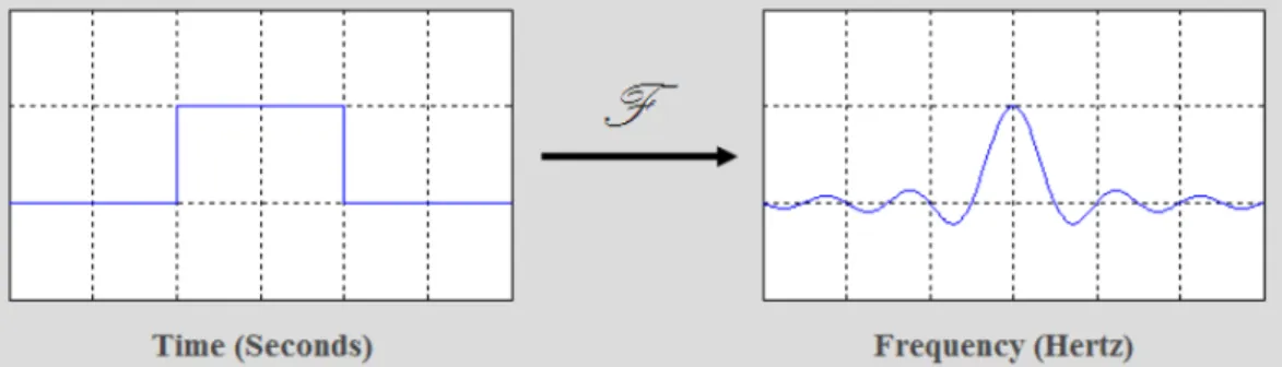
The Fourier Transform [22], named in honour of the French mathematician Jean Fourier, is an extension of the Fourier Series. Fourier Series are a way to re-write complicated periodic functions as a sum of simple waves, represented by sines and cosines. The Fourier transform decomposes a function of time (a signal) into sinusoids (the frequencies that make it up) and shows that any waveform can be re-written as the sum of sinusoidal functions. Fourier Transform extended the Fourier Series in a way that the period of the function can be infinite.

Figure 3.1: Fourier Transform - Source: thefouriertransform.com

The Fourier Transform is widely used in many areas, being of extreme importance in the pro-cessing of digital signals. Listening to digital music or watching TV are among the ordinary daily activities that could not be done without this Transform.

Hector uses several Fourier Transforms, and this will be one of the aspects that will try to be improved in the development of this dissertation.

There are multiple slightly different formulas to describe the Fourier Transform. All of them can be outlined as:

(32)

Figure 3.2: Fourier Transform summarised - Source: johndcook.com

Where m is 1 or 2π, σ is +1 or -1 and q can be 2π or 1. So, there are 8 potential definitions [23].

3.1.1 Discrete Fourier Transform

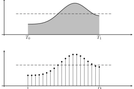
In order to compute the Fourier Transform on computers, one needs discrete values instead of continuous ones. Therefore, on computers, Discrete Fourier Transform (DFT) is used.

Figure 3.3: Discrete Fourier Transform and its inverse - Source: wikipedia.org

DFTs [24] algorithms are quite sluggish, their complexity is O(n2_{), in this way, on computers, is}

used Fast Fourier Transform (FFT) to calculate Fourier Transforms. FFTs [25] [26] are no more than a factorisation of the DFT matrix into a product of sparse factors with a complexity of

O(nlogn).

There are many algorithms to calculate FFTs, the most significant ones are going to be detailed further in this chapter.

(33)

3.2 FFTW

Fastest Fourier Transform in the West (FFTW) [27] is a C subroutine library for computing the Discrete Fourier Transform in one or more dimensions, of arbitrary input size, and of both real and complex data.

The first version was released in MIT by Matteo Frigo and Steven G. Johnson and is an open-source library, released under GNU General Public Licence [28], currently on version 3.3.8.

FFTW is the most widely known library for Fourier Transform computing and the one with the [29] best performance among all the free FFT software for CPU usage.

Among other interesting features, FFTW supports parallel transforms and it is portable to any platform with C compiler.

The library operates only on CPUs and is used in Hector to compute every Fast Fourier Transform the program has.

3.3 cuFFT

cuFFT - CUDA Fast Fourier Transform [30] is a library designed to provide high performance on NVIDIA GPUs. The library is an improvement from the FFTW, a library written in C language with the same purpose: computing the Fourier Transform.

The cuFFT library offers an interface for FFTs computing, it is a highly optimised and tested library that employs CUDA to take advantage of the parallelism of GPUs to drive fast and opti-mized executions of the Fourier Transform.

In addition to cuFFT, there is also cuFFTW library, a porting tool to enable FFTW users to start using NVIDIA GPUs with a minimum effort.

cuFFT data layout is compatible with FFTW and it supports the usage of multiple GPUs.

Currently, cuFFT is the library that presents the best performance to calculate Fourier Trans-forms [31].

3.3.1 cuFFT sample

cuFFT sample

// Memory allocations on GPU cufftDoubleReal * y_gpu ;

cufftDoubleComplex *Y_cuFFT ,* Y_gpu ; cufftHandle plan_forward_cuFFT ;

double * y_pinned ;

int n = 1000; // FFT size

// Pinned memory allocation on CPU // y_pinned - input array

// Y_cuFFT - stores the FFT output

cudaMallocHost ((void **) &y_pinned , n*sizeof(double));

cudaMallocHost ((void **) &Y_cuFFT , n*sizeof( cufftDoubleComplex )); // Fill array with dummy data

(34)

for (int i=0;i<n;i++) y_pinned [i] = 1.0*i; // Memory allocation on GPU

// y_gpu - FFT input Real array // Y_gpu - FFT output Complex array

cudaMalloc ((void**)& y_gpu , sizeof( cufftDoubleReal )*(n)); cudaMalloc ((void**)& Y_gpu , sizeof( cufftDoubleComplex )*(n));

int batch = 1; // batch size // FFT plan creation

// D2Z - Double Real to Double Complex

cufftPlan1d (& plan_forward_cuFFT , n, CUFFT_D2Z , batch ); // Copy FFT input array from CPU to GPU

cudaMemcpy (y_gpu ,y_pinned ,sizeof(double)*(n), cudaMemcpyHostToDevice ); // FFT execution

cufftExecD2Z ( plan_forward_cuFFT , y_gpu , Y_gpu );

// Blocks until GPU has completed all preceding requested tasks cudaDeviceSynchronize ();

// Copies FFT output to CPU

cudaMemcpy (Y_cuFFT ,Y_gpu ,sizeof( cufftDoubleComplex )*(n), cudaMemcpyDeviceToHost );

// Clean -up memory

cudaFreeHost ( y_pinned ); cudaFree (y_gpu );

cudaFree (Y_gpu );

cudaFreeHost ( Y_cuFFT );

3.4 FFTW vs cuFFT

Before starting to change the Hector code to make it seize the GPU capabilities, a small program was created to evaluate the feasibility of using cuFFT.

The program is pretty straightforward, it measures the execution time of the FFT on CPU and on GPU, and is also measured the copy time, from Host (CPU) to Device (GPU) and from Device to Host, in the conventional CUDA way and with pinned memory.

(35)

Laptop Server

Computer Asus P24440U DELL PowerEdge R740 Rack Server (Virtual Machine - VMware ESXi) CPU Intel Core i7-7500U - 3.5GHz Intel Xeon Silver 4112 - 2.60GHz 2 physical cores, 4 logical cores 4 physical cores, 8 logical cores GPU Nvidia GeForce 940MX Nvidia Quadro P6000

OS Linux Mint 18.3 sylvia Linux Mint 18.3 sylvia

RAM 12GB 8GB

GPU Memory 2GB 24GB Nvidia Driver Version 418.56 418.56 CUDA Version 10.1 10.1

Table 3.1: Computers Specifications

3.4.1 Pinned Memory

The data allocated by the CPU is pageable [32], so it cannot be accessed by the GPU directly, it must be transferred from the CPU to the GPU. For this purpose, CUDA allocates a temporary pinned host array and copies the pageable data to the pinned array and then transfers the data to the GPU, as described in figure 3.5.

Pinned memory operates as a “staging area” for the transfers, which delays the copy. To reduce the cost of the transfer, it is possible to allocate data directly in pinned memory.

One may think that if pinned memory makes the transfers quicker, then it should always be used, however, pinned memory needs to be used cautiously. First, the pinned memory perfor-mance relies on the device being used. Secondly, over-allocating pinned memory can reduce significantly the system performance by reducing the amount of physical memory available for the other programs and tasks. Naturally, this depends on the capabilities of the machine being used, so as the program that uses pinned memory itself. To be sure, both uses should be tested in order to determine which suits best for each scenario.

(36)

3.4.2 Ordinary Laptop

The first benchmarkings were done on the laptop.

The findings are displayed on the table 3.2 below. Fast Fourier Transforms are exceptionally fast operations, for that reason, to simplify and make the results easy to evaluate, the values on the table 3.2 are in milliseconds. To get the total time of cuFFT, one has to add the times of the copy to the GPU, time of cuFFT and the time to copy the result back to the main memory.

Size 1000 10000 100000 1000000 10000000 FFTW 8 91 1262 18787 261560 Copy to GPU 19 26 151 3899 46050 Pinned Copy 16 96 940 5568 46970 cuFFT 92 130 2620 5918 71646 Copy from GPU 21 59 481 4679 45727

Table 3.2: FFTW vs cuFFT benchmarking on laptop

Analysing the results, the usage of the GPU for FFT’s starts to be more advantageous for sizes larger than around 1000000. The pinned memory copies have intriguing outcomes, it is curious to note that pinned memory takes longer times than the pageable memory. [33] has shown that pinned memory fits better for large amounts of data, which could partially explain the results, however, the last test, done for a size of 10 million, can already be considered a large amount of data. The fact that the GPU device can interfere with the performance of the pinned memory cannot be overlooked, and the 940MX used for this benchmarking sustains a feeble performance.

3.4.3 Server with Nvidia Quadro P6000

The second benchmarking environment was the server equipped with the NVIDIA Quadro P6000 GPU and table 3.3 demonstrates the benchmarking results. The difference between both GPUs is highly evident. Already for time series with a length of between 10000 and 100000 the GPU outperforms the CPU. This is closer to the length of actual geodetic time series. Pinned memory, in this GPU, is always faster than pageable memory, even for small sizes, however, one must take into account once again the scale, that is in milliseconds. The time difference for small sizes is just substantial and would not be noticed on a smaller precision scale, despite that, the larger test cases, present significant time gains. In the last test, pinned copy is around 10 seconds faster than regular copy.

It is also notorious that the server, even having a CPU a little better than the laptop, presents worse results, which might be due to the virtualisation environment.

Size 1000 10000 100000 1000000 1000013 10000000 FFTW 11 117 1531 26011 151613 393425 Copy to GPU 22 34 204 1657 1704 17081 Pinned Copy 12 20 141 700 703 7366 cuFFT 56 78 100 554 3710 4763 Copy from GPU 15 20 97 691 701 6574

Table 3.3: FFTW vs cuFFT benchmarking on server

Considering the larger test, summing the times of the pinned memory copy plus the cuFFT exe-cution and the copy from GPU, the result is less than half of the time of the CPU FFT exeexe-cution. So, it is definitely worth to use a GPU to calculate Fast Fourier Transforms.

(37)

3.4.4 Hardware & FFTs Comparison

Figure 3.6 shows the last columns of Tables 3.2 and 3.3. It demonstrates the importance of a GPU to compute Fast Fourier Transforms. The results are in both cases (laptop and server with NVIDIA Quadro P6000) much faster on GPU than on CPU, even considering that the copies to and from GPU need to be added to the cuFFT execution time.

Another conclusion that can be drawn from the graph, is that FFTW (the CPU version) performs better on the laptop than on the server which could be explained by virtualisation of the device in use and processor kinds. Both processors do not have many differences, plus, adding the cost of virtualisation, makes the server slower to run the same Fast Fourier Transforms on CPU. The pinned memory copy is only faster than pageable copy on the server, on the laptop, it raises the copy time.

It is also conclusive that the distinction between CPU and GPU is tremendous, however, in this case, FFTs were executed with large sizes and inside a loop, which makes cuFFT worthy. It would therefore be meaningless to transform the code to CUDA for a easy single implementation of a Fast Fourier Transform, with tiny dimensions, once the gain in time would be imperceptible.

Figure 3.6: FFTW vs cuFFT & Laptop vs Server (Nvidia Quadro P6000)

3.4.5 Prime Numbers FFT

During the experiments conducted with the FFT libraries, was detected something peculiar, two near numbers need an extremely disparate time to execute. The FFT execution time depends on the number of the size. If the size is a product of small prime numbers, or not. For instance, an FFT of size 1000000 needs 26011 milliseconds to be computed on CPU and 554 on GPU, on the server. However, 1000013 (only plus 13) needs 151613 milliseconds on CPU and 3710 on GPU, which is about 500% slower in both cases. The reason behind is that the number 1000000 can be written as a product of small prime numbers. 1000000 = 26_{∗ 5}6_.

The explanation for this is due to the implementation of the FFT and cuFFT libraries. Both libraries use the Cooley-Tukey algorithm (3.4.6.1) to reduce the number of operations needed to optimise the performance.

(38)

3.4.6 FFTW and cuFFT algorithms

FFTW and cuFFT are the most optimized libraries available for the computation of FFTs [31], both libraries attempt to use the fastest existing algorithms to compute the Fast Fourier Trans-form. The algorithms used are almost the same for both libraries. These algorithms are going to be described in the next sections.

3.4.6.1 Cooley-Turkey algorithm

Cooley-Tukey algorithm [34] [35], named after James Cooley and John Tukey is the most common Fast Fourier Transform algorithm. It is based in the divide and conquer principle and expresses the DFT as a product of sparse building blocks, in other words, the Cooley-Tukey algorithm re-writes a DTF in smaller DFTs. The libraries implement radix-2, radix-3, radix-5, and radix-7 blocks, which means that if the size of the transform can be factored as 2a∗ 3b ∗ 5c ∗ 7d (where a, b, c, and d are non-negative integers), the transform has enhanced performance.

The decomposition in powers of two is the one that expresses the best performance, while greater prime numbers have worse performance, however, still O(nlogn).

When a number cannot be decomposed as product of prime powers, cuFFT uses Bluestein’s algorithm 3.4.6.2 and FFTW uses prime-factor algorithm 3.4.6.3, Rader’s algorithm 3.4.6.4, and a split-radix algorithm ??. These algorithms need more computations per output point than the Cooley-Tukey, which makes the latter faster and more accurate.

3.4.6.2 Bluestein’s Algorithm

Bluestein’s algorithm [36] [37], also known as chirp-z algorithm, is a Fast Fourier Transform algorithm that computes the Discrete Fourier Transform (and others) of arbitrary sizes by re-expressing the DFT as a linear convolution.

Differently from Cooley-Tukey algorithm, Bluestein’s can compute FFTs of prime and non-prime sizes, however, for prime sizes, Cooley-Tukey is much faster than Bluestein’s.

3.4.6.3 Prime-Factor Algorithm

Prime-factor algorithm [38], also called Good-Thomas algorithm is a Fast Fourier Transform algo-rithm that re-expresses the Discrete Fourier Transform of a size N = N1N2as a two-dimensional

N1∗ N2DFT only for the case where N1and N2are relatively prime numbers. Bear in mind that

two integers are relatively prime if the only positive integer that divides both is 1, and conse-quently, any prime number that divides one does not divide the other [39].

The two resulting minor transformations are then computed by other FFT algorithm, that can be Cooley-Tukey for example.

Prime-factor algorithm is slower than Cooley-Tukey once it works only for relatively prime num-bers and so, it is useless for sizes power of two, which are the quickest computed by Cooley-Tukey.

3.4.6.4 Rader’s Algorithm

Rader’s algorithm [40], named for Charles M. Rader, is a Fast Fourier Transform algorithm that computes the DFT of prime sizes by re-expressing the DFT as a circular convolution.

Rader’s algorithm is typically only used for large-prime base cases of Cooley–Tukey’s recursive decomposition of the DFT.

(39)

3.4.6.5 Split-Radix

Split-radix [41] is a variant of the Cooley–Tukey FFT algorithm that uses a blend of radices 2 and 4. It recursively expresses a DFT of length N in one smaller DFT of length N/2 and two smaller DFTs of length N/4.

Split-radix can only be applied when N is a number multiple of 4.

3.5 Welch’s method

In the introduction we mentioned that geodetic time series contain correlated noise and that this need to be included in the time series analysis to ensure realistic uncertainties for the estimated linear trend. In geophysical time series the temporal correlated noise has larger amplitude at the long periods than at the high frequencies. Therefore, the use of FFT which decomposes the noise into a sum of simple waves can be used to study the properties of the noise. In fact, only the square of the amplitudes is needed while the phase of the waves is ignored. This is called a power spectrum. A popular method to compute power spectra is the periodogram method of Philip Welch [42]. It is a method to estimate the power of a signal at different frequencies. Welch’s method divides the time signal into successive blocks, forming the periodogram for each block, then, this method applies a Fourier Transform and averaging for each block.

3.6 estimatespectrum

The first Hector program being converted to CUDA was estimatespectrum. estimatespectrum is a program to estimate the power spectral density from data or residuals (the difference between observations minus the estimated linear trend and additional offsets and periodic signals) using the Welch periodogram method. The program is written in C++ language and to estimate the power spectral density, it uses the Fourier Transform.

estimatespectrum was written using the library FFTW to perform the Fourier Transforms. This library is the most famous and among the best libraries to calculate Fourier Transforms in terms of performance.

The first step in making estimatespectrum executing the Fourier Transform on the GPU was to change it from using the FFTW to cuFFT, a library that came up to be the FFTW for GPUs, more specifically, for NVIDIA GPUs, through CUDA programming.

3.6.1 Estimate Spectrum - From CPU to GPU

In the beginning, transforming the use of CPU to GPU appeared to be easy, a straightforward shift to the API calls seemed to work at first glance, although it ended up not being the case. GPU programming is a completely distinct way of programming, and the documentation is quite terse. GPU programming is still not widely used, and to find information is difficult, as the CUDA developers community remains small and under development.

estimatespectrum used a way to calculate the Fourier Transform by executing a transform of real to complex values as many times as the number of segments given as input. This programming procedure works perfectly for the CPU version of estimatespectrum, once it makes n calls to the API and splits the data size for each call, making the FFTs size smaller, and consequently their execution faster. Although, programming for GPU is completely different. Making n calls to

(40)

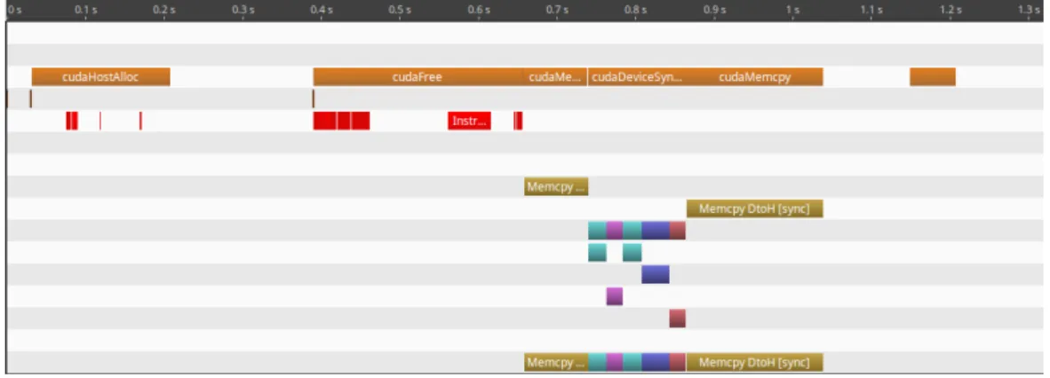
cuFFT is a way far from a good solution. GPU programming has a high cost on transferring data from/to GPU as one could perceive by analysing table 3.3, therefore, the fewer data moves the code needs, the faster the execution will be. In this program, as depicted on figure 3.7, most of the time spent executing the GPU code of estimatespectrum is precisely on the data transfers. In order to shorten transfers, the code was rewritten to execute only once the real to complex transform. Instead of smaller FFTs, CUDA code executes only a single one containing all the data. This way, multiple CPU/GPU copies are avoided, reducing them to only 2. One to copy from CPU to GPU, and the other to copy in an inverse way the result of the Fourier Transform.

Figure 3.7: Nvidia Visual Profiler - estimatespectrum execution with a dataset of 10.000.000 entries

NVIDIA Visual Profiler (NVVP) [43] is a cross-platform performance profiling tool that delivers feedback for optimising CUDA C/C++ applications. This usefull tool helps to identify performance bottlenecks, memory transfers, kernel launches and other API functions.

NVVP showed that the Fourier Transforms used on estimatespectrum do not need heavy compu-tation power from the GPU.

3.6.2 estimatespectrum - Workflow

Once the program reaches the section to compute the Fourier Transform, it starts by allocating memory on both CPU and GPU. On CPU, the memory is required to fill the array and to get the result of the transform. On GPU, the allocated memory has the purpose of receiving a copy of the data array and another array to save the transform result, the last one, is an array of

complex values.

On the CPU version of estimatespectrum, the data array was filled into portions of n size, 1 for each of the segments. On the GPU version, the array is filled once with all the data.

After allocating the memory required for the Fourier Transform and filling the array, data has to be copied to the GPU. When the data is in the GPU, the Fourier Transform can then be executed. On estimatespectrum, the desired transform is from real to complex type, and all the values have double size.

When the transform completes its execution, the resulting array of type real is copied from GPU to another array of the same size on CPU. Then, estimatespectrum maintains its own stan-dard execution flow, with a few fresh variations to adjust the software to the GPU variant, which executes the Fourier Transform only only once instead of the n times on the previous estimatespectrum version.

(41)

Figure 3.8: Fourier Transform workflow on estimatespectrum program

3.6.3 estimatespectrum - CPU vs GPU

After altering the estimatespectrum code in order to use the capacities of the GPU, it was essential to benchmark its results to figure out whether the implemented changes showed any advantage. The benchmark content is on the table 4.5 and the computer used for this benchmark was the laptop.

(42)

Noise size Segments Output CPU Output GPU Time CPU (s) Time GPU (s) 1,000 4 40.35 40.35 0.0041 0.2419 1,000 8 41.19 41.19 0.0039 0.2343 1,000 16 41.45 41.45 0.0038 0.2311 1,000 32 39.03 39.03 0.0038 0.2345 1,000 64 38.47 38.47 0.0043 0.2308 1,000 128 36.08 36.08 0.0051 0.2318 1,000 256 31.42 31.42 0.0051 0.2356 100,000 4 74.28 74.28 0.1715 0.3458 100,000 8 71.94 71.94 0.0932 0.3304 100,000 16 71.78 71.78 0.0861 0.3195 100,000 32 71.85 71.85 0.0837 0.3163 100,000 64 71.52 71.52 0.0848 0.3222 100,000 128 71.23 71.23 0.0837 0.3213 100,000 256 71.34 71.34 0.0808 0.3146 1,000,000 4 75.84 75.84 1.0747 1.3233 1,000,000 8 74.81 74.81 0.8903 1.2031 1,000,000 16 75.32 75.32 0.8228 1.1661 1,000,000 32 74.88 74.88 0.7916 1.1559 1,000,000 64 74.91 74.91 0.7722 1.0998 1,000,000 128 74.75 74.75 0.7710 1.1494 1,000,000 256 74.79 74.79 0.7603 1.0598 10,000,000 4 110.2 110.2 10.6721 11.5416 10,000,000 8 108.5 108.5 9.4353 10.0637 10,000,000 16 106.3 106.3 8.5330 9.3756 10,000,000 32 108 108 8.2151 9.1024 10,000,000 64 108.1 108.1 7.9363 8.8207 10,000,000 128 108.3 108.3 7.8248 8.9665 10,000,000 256 108.2 error 8.3638 -20,000,000 4 97.1 97.1 20.9583 23.2113 20,000,000 8 98.06 98.06 18.5839 20.0514 20,000,000 16 99.59 99.59 17.3342 18.8637 20,000,000 32 98.89 98.89 16.4541 18.0266 20,000,000 64 99.61 error 15.9948 -20,000,000 128 99.96 error 15.7427 -20,000,000 256 99.8 error 15.7068

-Table 3.4: estimatespectrum benchmarks

The program was executed with different noise sizes as input and different segments. Segments are no more than the blocks obtained from the division of the time signal by Welch’s method. A best description of this method can be found in 3.5.

The output of the program is always the same for both CPU and GPU variants of estimatespec-trum, which makes it possible to conclude that the inclusion of the CUDA code was properly done. As one can tell by analysing the table, sometimes the GPU variant presents error as out-put. This occurs because it is not possible to allocate the required size to execute the Fourier Transform on the used device. Two alternative measures could be taken in order to address this problem: split the transform execution into two or more segments or use a GPU with greater capabilities. As the table shows, the GPU is never faster than CPU and according to the figure 3.7, most of the time needed to run the program is spent copying memory between CPU and GPU, for this reason, the first possibility was disregarded, since splitting the transform execu-tion into porexecu-tions would require addiexecu-tional memory copies, which would increase the execuexecu-tion time of the GPU. Therefore, there was available for this dissertation a powerful GPU for which allocating more memory space would not be an issue.

(43)

The difference on the time execution between the two versions is merely substantial, although, in theory, one would expect a better performance on the GPU than on CPU. Multiple factors may explain why that does not occur, the most obvious one being that the size of the Fourier Transform and the number of its executions is not large enough in this program to justify the usage of a GPU. Other factors such as the benchmarking environment can explain these results. The experiments were conducted on a laptop which is not the ideal computer machine, and the GPU used is a low-range one. However, the CPU is still one the best available for laptops. Considering again the figure 3.7, it is clear that subtracting the time used on memory copies and freeing memory to the GPU runtimes would make the GPU executions faster than CPU.

3.6.4 estimatespectrum - Conclusions

After evaluating estimatespectrum, it became clear that more than 90% of execution time is being spent in input/output events, consequently, and considering the tiny FFT size and its reduced number of executions, there is not much to improve for estimatespectrum. The Fast Fourier Transform is already very fast on CPU, using a GPU, the FFT execution time is indeed faster but the time needed to copy from CPU to GPU and then from GPU back to GPU, led to the conclusion that the attempt to improve this program was in vain, since it is already well optimised. A significant amount of FFT executions would be necessary for the benefits to be noticed and estimatespectrum executes only one FFT.

estimatespectrum takes in average 2.03 milliseconds to execute the FFT on CPU, while on GPU it requires only 0.05 milliseconds (the copies between devices are not considered) for a size of 100000 points, which in real world is already a large size, so, it does not worth to spend time and efforts on making a program only 1.98 milliseconds faster.

Therefore, estimatespectrum was not even tested on NVIDIA Quadro P6000 GPU.

3.7 modelspectrum

Another important program for Hector that could be improved is modelspectrum. This program works as a validation software.

estimatespectrum was used before to compute the power spectral density of the residuals from an estimated trend and to verify if the chosen noise model for that trend is the correct. After run the estimatespectrum, one can use the program modelspectrum to compute the power spectral density of the estimated noise, to evaluate how well the modelled noise represents the reality (output of estimatespectrum). To do that, is used modelspectrum.

With estimatespectrum program, one can fit a power-law noise model to the spectral density estimates, then can construct plots like the ones on figure 3.9.

(44)

Figure 3.9: Power spectral density and fitted noise

The three primary kinds of noise are shown on the last chart. After generating these plots, one should manually evaluate if the chosen noise mode fits the power spectral density obtained by estimatespectrum program. In the showed cases, it perfectly fits, but how precisely the esti-mated noise model fits the periodogram? The answer can be obtained by using modelspectrum. This program acts basically as a validator that computes the confidence interval of the chosen noise for the power-spectrum obtained by estimatetrend. As input, it receives a noise model (the one chosen before) and the noise parameters, then it generates thousands of random time series and computes its power spectral density and fits the noise model, in order to evaluate how well it fits for each.

To determine accurately the fitness of the noise model, the number of simulations must be large, which will require several Fast Fourier Transforms (one per simulation). Thousands of simulations, as well as the size of the points for them, make the program sluggish, consequently, making it faster using the GPU, would be advantageous for Hector.

Figure 3.10: modelspectrum plot - KOSG station

The plot of a modelspectrum execution for a real case is shown on figure 3.10. It was used real data collected by a GNSS station, KOSG station, located at Kootwijk, Netherlands. The figure shows 3 red lines, the one in the middle represents the output of estimatetrend program 4.5 for the given noise parameters, the upper and lower lines represent modelspectrum output. The

(45)

blue dots are the estimated spectrum of the noise. The accuracy of modelspectrum is given by the percentage of blue dots between the upper and lower lines. In this case, more than 90% of the blue dots match this condition, therefore, this plot verifies that the fitted noise model (thick red line) indeed fits the real observed spectrum (blue dots).

3.7.1 modelspectrum CPU vs GPU

To improve the performance of this program, it was changed the way it performs the Fourier Transform. The GPU version of modelspectrum uses cuFFT instead of FFTW. In this program, thousands of FFTs are done for each execution, however, only one per Monte Carlo simulation. The benchmarks made for estimatespectrum clearly showed that cuFFT is faster than FFTW, however it did not make any difference for that case, once only one FFT is executed and the time gain is just a few milliseconds (and FFT on FFTW takes also a very short time, only some mil-liseconds for a normal real data size). So, multiplying these “few milmil-liseconds” by the thousands of executions, the final gain can be really promising.

The following table presents the tests made for a real case, once again, the data used is the one collected by the already mentioned KOSG station. For this station, there was available data with a size of 6387 points. Considering the small data size, it was tested with only 4 and 8 segments. The tests were run on both computers and runtime is displayed in seconds.

M.C. Simulations Segments CPU laptop CPU server GPU laptop GPU server 5000 4 13.85 14.87 15.32 9.28 10000 4 27.19 29.85 34.75 17.90 15000 4 39.17 44.66 47.19 26.42 20000 4 56.03 60.11 75.07 34.61 5000 8 14.08 13.81 20.38 10.45 10000 8 25.65 29.22 45.46 20.37 15000 8 40.99 44.21 79.36 29.28 20000 8 53.98 58.82 71.27 40.60

Table 3.5: modelspectrum benchmarks

Even for such a small case of only 6387 points, the benefits of using a GPU are evident. It is not worth to use the weak laptop GPU, once the CPU can have better results. On server, CPU once again has inferior results than laptop CPU, however, GPU exhibits the best performance in every single test. 3.11 chart helps to visualise the results.

Although not very different, the number of segments does not make a significant difference on the execution times.

The gain increases with the number of Monte Carlo simulations, nevertheless, the gain, even being around half of the time, does not seem to be remarkably high once the worst case takes only more than a minute, though, this is a benchmark that uses real data, the number of points can be either higher or even but not often, smaller. When higher, the gain becomes more relevant, when smaller, less, naturally. The benefit of using a GPU does not mean much to work with data from only one station, however, when Hector processes data from a network of stations, the benefits are more evident, instead of one minute, a network of stations can take up to hours to execute, depending on its size. Reducing the execution time by half, speeds-up modelspectrum in double.

The advantage of the GPU usage will soon be applied in a real context at SEGAL. Normally, 4 times a year, SEGAL researchers plot the power spectral density for all EPOS stations and its accuracy. This plots are publicly available atgnssproducts.epos.ubi.pt. Considering only the

(46)

smaller time gain using a GPU, 4 seconds, which occurs for the 5000 simulations case (which is the number of simulations being used by the researchers due to offering a satisfactory performance for the time needed), a gain of only 4 seconds per modelspectrum execution will have a major time reduction in the whole context. There are around 700 stations and for each there are East, North and Up coordinates to compute. Every station is part of 3 networks (UGA, INGV and BFKH). In this way, 700∗ 3 ∗ 3 = 6300 executions are needed. The total gain in seconds is given by multiplying 4 seconds by 6300 executions, 4∗ 6300 = 25200. 25200 seconds are exactly 7 hours, which will be the gain that SEGAL researchers will benefit from upon the next creation of plots. Soon, EPOS will have around 3000 stations, which reinforces the importance of using a GPU.

Figure 3.11: modelspectrum comparison for 20000 simulations - KOSG station, Kootwijk, Netherlands Orange - laptop, Green - server

3.7.2 Monte Carlo Simulation

Monte Carlo simulations, named after the gambling hot spot in Monaco, are statistic compu-tational algorithms, usually used to predict outcomes by repeating massively simulations using randomness to solve heuristically problems that might be deterministic.

Monte Carlo simulations are widely used in many areas, from finance to medicine and in the case of modelspectrum they help to determine the accuracy of a noise model by generating thousands of synthetic data using FFTs and Welch’s method 3.5 to calculate the power spectrum, which also uses FFTs. The usage of cuFFT library instead of FFTW is the reason behind the decrease in execution time of Monte Carlo simulations and hence, modelspectrum program.

3.8 Summary

The purpose of the events described in this chapter was to improve the performance of esti-matespectrum and modelspectrum, even though these are not Hector’s slowest programs, a reduction of the execution time would be very appreciated.

Use of GPU for time series analysis