On credit score models

M

ASTER

FINANCE

M

ASTER

´

S

F

INAL

W

ORK

PROJECT

ON

CREDIT

SCORE

MODELS

LAURA ARGOMANIZ

M

ASTER

FINANCE

M

ASTER

´

S

F

INAL

W

ORK

PROJECT

ON CREDIT SCORE MODELS

By Laura Argomaniz

S

:

Paulo Martins Silva

Paulo Santar Ferreira

Acknowledgements

Aos meus pais, a quem devo tudo o que tenho e tudo o que sou. Sortuda por ter a estrela mais brilhante do céu e o meu maior pilar na terra. Estou eternamente agradecida pelas “ferramentas para a vida” que me foram proporcionadas e pelo amor e carinho desmedido ao longo destes 25 anos.

Aos meus irmãos, por de certa forma terem tornado nesta irmã mais velha uma pessoa persistente e acompanhada para sempre.

À minha familia.

Ao meu orientador, Prof. Doutor Paulo Silva por me ter sempre mostrado o caminho, pela sua disponibilidade, conselhos e confiança neste trabalho.

Ao meu diretor, Dr. Paulo Ferreira, por apostar em mim todos os dias e disponibilizar-se sempre que o foi preciso, extenso à equipa de Análise de Crédito da MBFS-PT.

Um agradecimento muito especial ao Ricardo, por me ter acompanhado 24/7 e pelo seu apoio incondicional.

Por último, às pessoas que me acompanharam diaramente neste percurso, pelos conselhos e partilha de experiência inigualável, Cátia Dias e Prof. Doutor Carlos Geraldes.

Abstract

This study intends to model the Probability of Default (PD) of an American credit database. The logit model was used in order to determine the PD threshold that presents higher profits. The database contemplated 338.909 terminated loans lent to private individuals, consumer oriented, and 139 variables. From the rough data we reduced the number of variables to the most significant, according to the statistical tests computed in SPSS.

By the principle of parsimony two models were considered and the chosen model was the one that presented higher profits for the Financial Institution.

JEL classification: C52, C55,G11, G21, G40.

Keywords: Credit Risk, Generalized Linear Models, Logit, Scorecard, Discriminant Analysis, Calibration, Probability of Default, Credit Risk Management.

Resumo

Este estudo tem como objetivo modelar a probabilidade de incumprimento de uma carteira de crédito americana. Para tal, foi utilizado o modelo logit para apurar a probabilidade de incumprimento refêrencia para aceitação de crédito que supõe maior rendimento à Instituição Financeira. A Base de Dados recolhe informação de 338.909 empréstimos terminados, concedidos a particulares, destinados ao crédito ao consumo, e 139 variáveis, posteriormente reduzidas de acordo com o seu nível de significância, apurado nos testes estatítsticos realizados com o programa SPSS.

Pelo principio da parsimónia foram considerados dois modelos e o modelo escolhido foi o que apresenta comparativamente maior rendimento à Instituição Financiera.

Palavras-Chave: Risco de Crédito, Modelo Linear Generalizado, Logit, Scorecard, Discriminação, Calibração, Probabilidade de Incumprimento, Gestão do Risco de Crédito.

Table of Contents

1. Introduction 6

2. Credit Risk 7

2.1 Measuring Credit Risk 8

2.2 Generalized Linear Models 10

2.3 Literature Review 12

3. Methodology 15

4. The Data 21

5. Estimated model and results 22

5.1 Logistic regression 22

5.2 Model Validation 24

5.3 Accuracy 25

5.4 Calibration 26

5.5 Model Comparison 27

6. Application to a loan portfolio 28

7. Conclusions 30

8. Bibliography 30

Table 1 - Summary of the most common link functions ... 12

Table 2 - Model Comparison ... 27

Table 3 - Financial measures of each model ... 29

Table A.4 - Descriptive Analysis of Data ... 36

Table A.5 - Replacement of missing values mths_since_last_delinq ... 36

Table A.6 - Replacement of missing values mths_since_last_record ... 36

Table A.7 - T-Test Paired Sample ... 37

Table A.8 - Multicollinearity for variable loan_status (VIF) ... 37

Table A.9 - Model 1 Block 0 (Baseline model) ... 38

Table A.10 - Model 1 Variables in Equation ... 38

Table A.11 - Model 1 Omnibus test of model coefficients ... 38

Table A.12 - Model 1 Summary ... 38

Table A.13 - Model 1 Classification Table ... 39

Table A.14 - Model 1 Variables in Equation ... 39

Table A.15 - Model 1 Bootstrap ... 40

Table A.16 - Model 1 Group Statistics ... 41

Table A.17 - Model 1 Test Equality of Group Means ... 42

Table A.18 - Model 1 Eigenvalues ... 42

Table A.19 - Model 1 Wilk's Lambda ... 42

Table A.20 - Model 1 Standardized Canonical Discriminant Function Coefficients... 43

Table A.21 - Model 1 Structure Matrix ... 44

Table A.22 - Model 1 Classification Results ... 44

Table A.23 - Model 1 AUC... 45

Table A.24 - Model 1 Hosmer and Lemeshow Test for 338.909 subjects and 1.000 subjects ... 45

Table A.25 - Model 2 Block 0 (Baseline model) ... 46

Table A.26 - Model 2 Classification Table ... 46

Table A.27 - Model 2 Summary ... 46

Table A.28 - Model 2 AUC... 47

(1) Linear predictor ... 11

(2) Logit link function ... 12

(3) Logistic regression ... 18

(4) Probability function ... 18

(5) Variance inflation factor ... 18

(6) Sensitivity ... 20

(7) Specificity ... 20

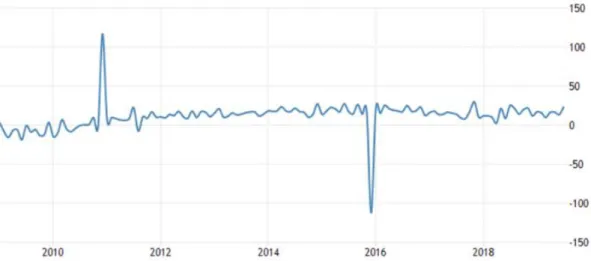
Figure A.1 - 10y data for consumer credit market in US ... 34

Figure A.2 - Forecast for consumer credit market in the US ... 35

Figure A.3 - Household income distribution US 2017 ... 35

Figure A.4 - Model 1 ROC Curve ... 45

6

1.

Introduction

Risk is an intrinsic event in every decision that is made in a daily basis. If risk wouldn’t be a subjacent consequence to every choice that we make, then decisions would be very easy.

Credit risk comes along in every lending/borrowing performed by Financial Institutions to consumers, and it accounts for the loss that the financial institution bears if the borrower does not comply with the agreement. Such agreement is in the form of a contract and states the repayment of a loan amount in a scheduled period.

Such action has become essential for the reach of increasing profits pursued by financial institutions and over the years consumer credit market has surpassed expectations in terms of value.

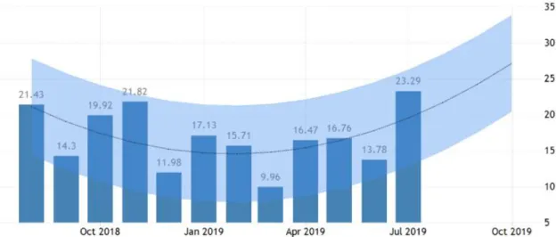
Specifically, in the United States, consumer credit market went up by USD 23.3 billion in July 2019 the most in a year, exceeding the expected growth of a USD 16.1 billion rise. Revolving credit including credit card borrowing climbed USD 10 billion; non-revolving credit including loans for education and automobiles rose USD 13.3 billion, after a USD 14.0 billion increase in the previous month. Year-on-year, consumer credit growth accelerated to 6.8 percent in July from 4.1 percent in June. Furthermore, consumer credit in the United States averaged 4.48 USD Billion from 1943 until 2019, reaching an all-time high of 116.79 USD Billion in December of 2010.1

Apart from the observed and unquestionable growth of consumer credit market, forecasts show that the trend is upwards and by October 2019 the value is expected to be at 34 USD Billion2_.

1 _{Figure A.1 – 10y credit data for consumer credit.}

7

As a counterpart of such growth, indebtedness of American families has been very present in credit history such as stated in works of Niu (2004) and Siddiqi (2006) which empirical studies rely on the importance that risk management of consumer lending plays against issues in consumer credit market. Such policies should ensure that every consumer has the credit for which it presents financial ability to repay. For that purposes, credit systems, as scorecards, are crucial in order to determine the scoring of a consumer and the default probability associated with it, that the financial institution is willing to accept.

It is important to note that there’s a difference between the risks that are present in the market, and that there are different ways to deal with each of them. It is possible to identify systemic risk and credit risk. Systemic risk is known as the collapse of the entire financial system and it is faced by governments with effective laws and regulation or optimal policy, (Saunders & Allen, 2002). What concerns credit risk, early development started with the work of Durand (1941), that gathered data of 7,200 individual loans, having good and bad repayment record, to apply statistical measures in order to define which of the characteristics had major weight in determining the default of a consumer. Such work had later developments made by Hand & Henley (1997) who studied the statistical methods used in the industry to predict credit risk.

The purpose of this study is to determine the principal factors leading to a higher probability of default of a consumer loan from an American database, through the construction of a credit model and then determine the threshold for acceptance of a probability of default (PD) in order to manage the profitability of a loan portfolio.

2.

Credit Risk

Credit risk is the probability of losing money derived from the lack of repayment of a conceded financial obligation, regardless the causes of the event. In the action of lending/borrowing money, there are always two parts, the lender (financial institution) and the customer/consumer. The financial institution

8

disposes the amount of money needed and expects its repayment according to the contract established, and a rate of return that should compensate for the risk incurred for providing liquidity. In the counterpart, the customer needs the liquidity and is responsible for the repayment plan, stated at the beginning of the contract. Facing the inability of repayment of a customer, there are three types of situation that can derive: insolvency, default and bankruptcy (Bouteillé & Coogan-Pushner, 2013). In the first one, insolvency, it is implied the lack of income from the customer, normally when the financial obligations exceed its assets; default, is the situation of non-meeting the financial obligation, that can derive from different situation. Third, bankruptcy, is when the default situation must be legally solved through the intervention of a court and the customer will be identified to a liquidation process through prioritizing its debtors and paying according to the court’s decision.

Loaned money; Lease obligation; Receivables; Prepayment for goods or services; Deposits, Claim or contingent claim on asset and derivatives as swaps or foreign-exchange futures, are the transactions that according to Bouteillé & Coogan-Pushner (2013) create credit risk. For the purpose of this study, our focus is on credit risk subjacent to loan of money.

The key point to credit risk, is that it is controllable and if well managed the losses can be minimized. To achieve it, it is crucial that institutions that are more exposed to credit risk (banks, asset managers, hedge funds, insurance companies and pension funds), follow models or guidelines to evaluate a customer and the risk present in the operation, and the action taken in case of default.

2.1

Measuring Credit Risk

Given the growth and large increase of the financial sector worldwide, mainly due to the concession of credit from Financial Institutions and given the remarkable impacts in international currency and banking markets (failure of

9

Bankhaus Herstatt in West Germany), Basel Committee3 was funded. Funded by the Central Bank Governors of the group of ten countries in 1974, such organization was pledged to strengthen financial stability by improving banking supervision and to serve as a convention for regular cooperation between its member countries, in order to regulate and to control inherent risks of the financial systems.

The first measure was to ensure supervision, foreseen in the “Concordat”. This paper was issued in 1975 and set out principles for sharing supervisory responsibility for banks, foreign branches, subsidiaries and joint ventures between host and parent supervisory entities. After some amendments and revisions to the initial document, several papers were released in the following years, and with the objective of achievement capital adequacy, Basel I was implemented. It was known as the Basel Capital Accord and pretended to struggle against the deterioration of the capital ratios of the main international banks. This resulted in a broad consensus on a weighted approach to the measurement of risk, both on and off-balance sheet.

In 1999, the Accord was replaced by a new proposal issued by the Committee. This new regulation was known as the Basel II and it comprised 3 pillars:

• Pillar 1: minimum capital requirements for credit, market and operational risk.

• Pillar 2: supervision process of capital requirements and an assessment of capital sufficiency considering all risks faced is performed.

• Pillar 3: broader detail in information released publicly (including risk models), through a market discipline annual document. This concern was translated in Market Risk.

Specifically in the paper Range of Practice in Bank’s Internal Rating Systems published by the Basel Committee on Banking Supervision (2000), and aiming the consistency of credit measurement, the institution spotlights the importance of the use of statistical tools such as scorecards, to measure the degree of

3 _{BIS (2019). About the BCBS. History of the Basel Committee. Available from:}

10

reliance on qualitative and quantitative factors. Statistical tool is exemplified using credit scoring models. The following steps are determined for the construction of such models:

1. Identification of the financial variables that appear to provide information about probability of default.

2. Using historical data of a sample of loans considered, an estimation of the influence of each of the identified variables in an eventual incidence of default is determined.

3. Estimated coefficients are then applied to data for current loans to arrive at a score that is indicative of the probability of default.

4. Score is converted into a rating grade.

Later, as a response to the financial crisis (2007-2009), known as the subprime crisis, Basel III was outlined and implemented. The crisis was mainly driven by too much leverage and inadequate liquidity buffers accompanied by poor governance and risk management, (Walter, 2010). This regulation was focused in the capital requirements of commercial banks, liquidity risk measurement, standards and monitoring by enhancing the previous rules stated by Basel II.

The last reform was in 2017, with the release of new standards for the calculation of capital requirements for credit risk, credit valuation adjustment risk and operational risk. The final reform also includes a revised leverage ratio, a leverage ratio buffer for global systemically important banks and an output floor, based on the revised standardized approaches, which limits the extent to which banks can use internal models to reduce risk-based capital requirements.

2.2

Generalized Linear Models

The Generalized Linear Model (GLM) derives from the normal linear model introduced in the XIX century by Legendre and Gauss, being this the dominant model until mid-XX century. Despite its extended use, there were situations for which this model was not the most appropriated, which lead to the development of non-linear models. Examples of these transformations are the logit model

11

(Berkson, 1944) and the probit model (Bliss, 1935). Nelder and Wedderburn (1972) resumed the models and a unified and broader class of GLM appeared.

The GLM acts as an extension of the normal linear model in which the relationship between the linear combination of explanatory variables (linear predictors) and the dependent variable (Y) is specified in a broader sense, which permits other distribution apart from the normal to model the response of Y. Any distribution to model the response of Y, has the form of an exponential function and the most used are Normal, Binomial, Poisson, Gamma and the

Inverse Gaussian distribution, (Turkman & Silva, 2000).

A generalized linear model is made up of a linear predictor

𝜂_𝑖 = 𝛽₀+ 𝛽₁𝑥_𝑙𝑖+ ⋯ + 𝛽_𝑝𝑥_𝑝𝑖 (1)

And two functions:

➔ A link function that describes how the mean, 𝐸(𝑌𝑖) = µ𝑖, depends on the

linear predictor 𝑔(𝜇_𝑖) = η𝑖.

➔ A variance function that describes how the variance, 𝑣𝑎𝑟(𝑌_𝑖) depends on the mean 𝑣𝑎𝑟(𝑌𝑖) = ∅𝑉(𝜇) , where the dispersion parameter ∅ is a

constant.

The linear predictor (η_𝑖) is a linear regression that contains the independent variables used in the model, X, and unknown parameters, 𝜷. Then η, can be expressed as:

𝜂 = 𝑿 𝜷

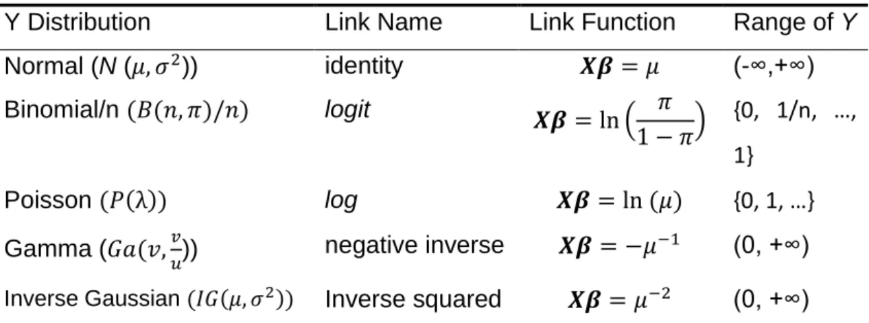
The link function stands as the relationship between the linear predictor and the mean (𝜇) of the distribution. As previously described, those functions belong to the exponential-family functions and they are known as the canonical link function. Table I summarizes the most common link functions.

12

Table 1 - Summary of the most common link functions

Y Distribution Link Name Link Function Range of Y

Normal (N (𝜇, 𝜎2)) identity 𝑿𝜷 = 𝜇 (-∞,+∞) Binomial/n (𝐵(𝑛, 𝜋)/𝑛) logit _{𝑿𝜷 = ln (} 𝜋 1 − 𝜋) {0, 1/n, …, 1} Poisson (𝑃(λ)) log 𝑿𝜷 = ln (𝜇) {0, 1, …} Gamma (𝐺𝑎(𝑣,𝑣 𝑢)) negative inverse 𝑿𝜷 = −𝜇 −1 _{(0, +∞)} Inverse Gaussian (𝐼𝐺(𝜇, 𝜎2)) Inverse squared 𝑿𝜷 = 𝜇−2 (0, +∞)

As our variable is a Yes/No (Dichotomous), Y∼ Binomial (𝑛_𝑖, 𝑝_𝑖), chosen link function is the logit, and its linear predictor is the following:

𝜇

= 𝜋

=

1+𝑒−𝜂𝑖 (2)

For the estimation of the unknown parameters 𝛽_𝑖 in the logistic regression, the maximum likelihood estimation (MLE) is used (Turkman & Silva, 2000).

2.3

Literature Review

When society begun to rely on financing to support its lifestyle and borrowing/lending became an every-day transaction, financial institutions only relied in experts to grant credit. Apart from the lack of a proper model, it was depending on humans and subjectivism was inevitable, meaning that the lending/borrowing decision was biased. Somerville & Taffler (1995) worked in the tendency for pessimism that bankers showed and pointed out the necessity of a more objective procedure instead of subjective approaches. This requirement was the driver for the appearance of different approaches to credit scoring and among them the most used ones were: (i) linear probability model, (ii) the logit model, (iii) the probit model and the (iv) discriminant analysis model. Among all research, the two models that prevailed in working papers were discriminant analysis and logit analysis.

13

The first development in discriminant analysis model was made by Altman, Haldeman, & Narayanan (1977) with the creation of the known ZETA discriminant model, that was an improvement of the previous Altman’s five variable model (Altman, 1968). The objective of the model was the classification of loan borrowers into repayment and non-repayment by deriving a linear function between accounting and market variables. Later, Scott (1981) developed a theoretical sound approach and concluded that the Zeta model approximates its theoretical bankruptcy construct.

Similarly, logit analysis predicts the probability of a borrower’s default taking into consideration accounting variables, assuming that the probability of default is logistically distributed, constrained to fall between 0 and 1. West (1985) used the logit model to assess the financial condition of Financial Institutions (FI) and to determine the probability of default of each one. Platt & Platt (1991) used the

logit model to test whether industry relative accounting ratios were better

predictors of bankruptcy than the firm specific accounting ratios. The study showed that industry relative accounting ratios gave better results that the specific firm ratios.

Despite the effectiveness verified worldwide of the credit-scoring models, they have been subject to criticisms: lack of adjustment to market values and its rigid principle of linearity. Some of the models against those assumptions were:

• “Risk of Ruin” bankruptcy models based on the relationship of a firm’s assets (A) and obligations (B) at bankruptcy time and market liquidation, in the sense that such event occurs when the value of A falls below B. Kealhofer (1997) showed that it is possible to calculate a firm’s expected default frequency given any initial values of A and B and a calculated value for the dispersion of A overtime (𝜎_𝐴).

• Models that seek to impute implied probabilities of default from the term structure of yield spreads between default free and risky corporate securities, were the second class that appeared first in Jonkhart (1979).

14

• Mortality rate model of Altman (1988, 1989) and the aging approach of Asquith, Mullins, & Wolff (1989). The model was capital market based and was used to derive actuarial-type probabilities of default from past data on bond defaults by credit grade and years to maturity. The application of these models was majorly by rating agencies (e.g. Moody’s, 1990; Standard and Poor’s, 1991). The downside of these models was the quantity of loan data that seen as not enough to reach such conclusions. According to Altman & Saunders (1998) this weakness can be seen as the reason for which so many initiatives among the larger banks in USA started a shared national data base of historic mortality loss rates on loans.

• The application of neural network analysis to credit risk classification problem can be seen as the fourth developed model. In this model the linearity of probability of default is not mandatory and then it is translated in a non-linear discriminant analysis where the potential correlation among predictive variables of the prediction function. Examples of applications of the model are Altman (1994) and Coats & Fant (1993) that used it to corporate distress prediction in Italy and Trippi & Turban (1997) in the US.

According to Hao, Alam, & Carling (2010) given the above classes of models that appeared in substitution of the traditional credit-scoring, three broad classifications, according to the basis and assumptions inherent to each of them, can be determined: (i) structural models, (ii) individual-level reduced-form models and (iii) portfolio reduced-form models.

For the purpose of this study, we are only going to focus on individual-level reduced-form models - the credit scoring models. The first use and appearance of these type of models was in 1968 with the 5 variable model that Altman developed. Altman & Narayanan (1997) found that financial ratios that measured profitability, leverage and liquidity were the basis of the credit scoring models. Further developments were done by Altman & Saunders (1998), when these types of models became very significant at the time of lending. In the beginning

15

of 2000, studies on these models decreased and the developments possible to track are Jacobson & Roszbach (2003) with the bivariate model proposed to calculate portfolio credit risk. Lin (2009) worked with neural network and constructed three kinds of two-stage hybrid models of logistic regression (ANN) and Altman (2005) focused in the emerging markets by constructing a score model for emerging corporate bonds. Luppi, Marzo, & Scorcu (2008) study the application of a logit model to Italian non-profit SMEs and found that the traditional accounting-based credit scoring model had less explanatory power in non-profit firms that in for-profit firms.

3.

Methodology

Under the Binary Regression Model, apart from the logit link function already presented, there’s the probit model, being these two the most commonly used approaches to estimating binary response variables.

Although they are two different models, the differences between the two are hard to define. Chambers & Cox (1967) found that it was only possible to discriminate between the two models when sample sizes were large and certain patterns were observed in the data.

Given the equivalence between the models, in this study we selected the logit model, as it is the most versatile of the two: “It is simple and elegant analytical properties permit its use in widely different contexts and for a variety of purposes” (Cramer, 2003).

Credit scoring databases are often large, with more than 100.000 applicants measured on more than 100 variables, especially when databases are behavioral, once that they gather all the past information and history of every subject.

Given the constrains from EU General Data Protection Regulation (GDPR) – the most important change in data privacy regulation in 20 years - enterprises had to manage data in a very restricted method. Thus, it was very difficult to find a local database that could be used for academic purposes. Therefore, the

16

database chosen for this study was extracted from the LendingClub4 (LC). It is an American database, that can present differences from local behaviors or economic conditions, that gathers all the issued loans and current portfolio of 338.909 subjects, lent between 2012 and 2018, characterized by 139 variables. In this section, the methodology carried out to determine the linear predictor that explains the default variable (loan_status) is presented together with the respective analysis to determine the level of reliability and applicability of the estimated model.

A default probability will be derived and then applied to a loan portfolio in order to determine the threshold for acceptance of credit that accounts for the higher profitability.

The response variable, loan_status, has the following possible outcomes:

𝑌 = {1 if loan is at default

5 _{or charged off}6

0 𝑖𝑓 𝑙𝑜𝑎𝑛 𝑖𝑠 𝑓𝑢𝑙𝑙𝑦 𝑝𝑎𝑖𝑑7

Throughout this work, we used the software SPSS for the required statistical tests, and the level of significance (p-value) in the analysis was set at 0.05.

Data treatment

As the goal is to model consumer credit default probabilities, the first adjustment was to filter the purpose of the loan and reduce the database to (i)

4 _{Lending Club is a US peer-to-peer lending company, headquartered in San Francisco,}

California. It was the first peer-to-peer lender to register its offerings as securities with the Securities and Exchange Commission (SEC), and to offer loan trading on a secondary market. Nowadays LendingClub is the world's largest peer-to-peer lending platform. The LendingClub. Lending Club Loan Data. Available from:

https://www.kaggle.com/wendykan/lending-club-loan-data [Accessed: 15/04/2019].

5 _{LC classifies as default loans for which borrowers have failed to make payments for an}

extended period.

6 _{LC classifies as charged off loan hen there is no longer a reasonable expectation of further}

payments.

7 _{Loan has been fully repaid, either at the expiration of the 3- or 5-year year term or as a result}

17

car, (ii) credit card, (iii) home improvements, (iv) major purchases, (v) wedding and (vi) vacation, loans, each one of the above classes representing a dummy variable (Yes/No). Then, there were some variables that were eliminated either because they resulted from the combination of others, to avoid correlation, or they did not have economic meaning. The third step was to categorize the variables according to their nature and the following four categories were identified: (i) loan conditions and economic characteristics; (ii) level of indebtedness and financial capability of an applicant; (iii) historical data and credit behavior. Apart from the above categories, there’s the dependent variable, loan_status, and a computed variable, credit_life_years, to test whether the years of credit management have weight in a possible default event.

Missing Values

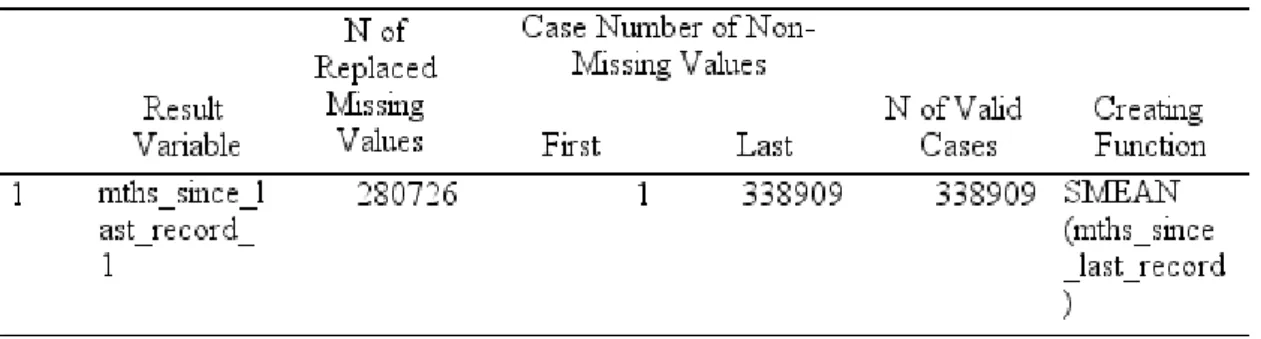
It is important to check if there are any values that are not expected or if there are any missing values that can bias our conclusions or even prevent us to carry out some tests/analysis. After a descriptive analysis (Table A.4), it was detected that there were some variables that presented missing values8 _{and the}

method to correct it was the Replace Missing Values of SPSS software.

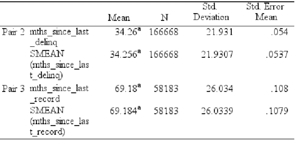
The replacement method used was Replacement by the mean9 and afterwards a T-Test Paired Sample10 _{was carried out to understand the level of deviation}

between the new variables and old variables. As shown in Table A.11, there is no difference between the new variables (_1) and the old variables, so the new variables were considered to the analysis of the model instead of the old that presented missing values.

Logistic Regression

The binary logistic regression (logit) is the function that is going to determine the coefficients (𝛽_𝑖) of the independent variables in the equation, and

8 _{Output results in Table A.4 – Descriptive analysis of data.} 9 _{Output results in Tables A.5 and A.6.}

18

the level of significance (p-value) that each of them presents, to determine if they have enough explanatory power to predict a default situation.

After identification of the set of significant variables, the regression equation can be computed, and a level of risk associated with each event will be possible to calculate.

The regression equation:

𝜇𝑖 = ℎ(𝛽0+ 𝛽1𝑋1+ ⋯ + 𝛽𝑛𝑋𝑛) = 1

1+𝑒−𝜂𝑖 (3)

Where

𝜇_𝑖 = log (𝑜𝑑𝑑𝑠_𝑜𝑓_𝑑𝑒𝑓𝑎𝑢𝑙𝑡 )

And the probability of default is given by

𝑃(𝐷𝑒𝑓𝑎𝑢𝑙𝑡) = 𝜋𝑖 (4)

Multicollinearity diagnosis

Correlation in regression analysis can adversely affect the regression results that can lead us to biased conclusions and decisions. Its diagnosis can be made looking at the Variance Inflation Factor (VIF) (Tibshirani, James, Witten, & Hastie, 2013). VIF is calculated for all predictors, regressing them against every other predictor in the model.

It is calculated through the following formula:

𝑉𝐼𝐹(𝛽) = 1

1−𝑅_{𝑥𝑗|𝑥−𝑗}2 (5)

Where 𝑅_𝑥2_{𝑗|𝑥−𝑗} is the 𝑅2 from a regression of 𝑋𝑗 onto all the other

predictors. If 𝑅_𝑥2_{𝑗|𝑥−𝑗} is close to one, then collinearity is present, and so the VIF will be large.

19

As a rule of thumb for VIF interpretation, there are the following levels, (Tibshirani et al., 2013):

1. Not correlated

2. Between 1 and 5 we are in the presence of moderate correlation. 3. Greater than 5 indicates high level of correlation.

Model Validation

Regression analysis is useful when the estimated model can be extended to a population sample in order to predict outcomes in new subjects. To determine if the estimated model is a good fit, a goodness-of-fit analysis or model validation

analysis (Harrell, Lee, & Mark, 1996) must be performed.

To perform a model validation a sample must be chosen, and as sometimes it is impossible to obtain a new dataset to test the estimated model, an internal validation can be computed. According to Giancristofaro & Salmaso (2003), there are four most accredited methods for internal validation; (i)

data-splitting; (ii) repeated data-data-splitting; (iii) jack-knife technique and (iv) bootstrapping.

After deep analysis of the techniques used for validating a logistic regression,

bootstrapping is referred as the most used, and therefore, it is the method chosen

for model validation.

Bootstrapping is a method of internal validation that consists in taking a large

number of simple random samples with replacement from the original sample, (Harrell et al., 1996). It computes estimates for every 𝛽𝑖 parameter and calculates

confidence intervals at 95% along with their significance (p-value).

Accuracy and calibration

A complete evaluation of the fitting of an estimated model, should contemplate both accuracy and calibration (Hosmer & Lemeshow, 2000).

Accuracy refers to the ability of the model to “separate subjects with different

responses” (Harrell et al., 1996). Considering a logistic regression where two types of outcomes are possible, one group is called positive and the other group

20

is called negative. Through a discriminant analysis it is possible to determine the extent at which the two events are differentiated between the two groups.

After performing a discriminant analysis in SPSS, one of the resulting tables is classification table from where we can derive sensitivity and specificity measures of a model and then, using the model’s regression equation, we can calculate the probabilities for positive events and display it in a Receiver Operating Characteristic (ROC) curve. This curve plots the probability of correctly classifying a positive subject (sensitivity) against the probability of incorrectly classifying a negative subject (one minus specificity).

𝑆𝑒𝑛𝑠𝑖𝑡𝑖𝑣𝑖𝑡𝑦 = (𝑃𝑟𝑒𝑑+,𝑂𝑏𝑠+)

(𝑃𝑟𝑒𝑑+,𝑂𝑏𝑠+)+(𝑃𝑟𝑒𝑑−,𝑂𝑏𝑠+) (6)

𝑆𝑝𝑒𝑐𝑖𝑓𝑖𝑐𝑖𝑡𝑦 = (𝑃𝑟𝑒𝑑−,𝑂𝑏𝑠−)

(𝑃𝑟𝑒𝑑+,𝑂𝑏𝑠−)+(𝑃𝑟𝑒𝑑−,𝑂𝑏𝑠−) (7)

The larger the area under the ROC curve (AUC), the more the model discriminates. The more upward-left the curve is shaped the better for accuracy results. Although there’s no perfect value determined for the AUC, there’s a rule of thumb that can be considered (Hosmer & Lemeshow, 2000):

• 𝑅𝑂𝐶 < 0.5, model has negative accuracy, worse than random. A model that has this feature, tends to classify positive subjects as negative and negative subjects as positive (Harrell et al., 1996).

• 𝑅𝑂𝐶 = 0.5, this suggests no accuracy – the same as flipping a coin. • 0.5 < 𝑅𝑂𝐶 < 0.7, suggests poor accuracy.

• 0.7 ≤ 𝑅𝑂𝐶 < 0.8, considered acceptable accuracy. • 𝑅𝑂𝐶 ≥ 0.9, considered an outstanding accuracy.

Calibration is a measure of how close the predicted probabilities are to the

observed rate of positive outcome (Harrell et al., 1996). Given the research that has been made, the most used test for calibration is the statistic produced by Hosmer & Lemeshow (1980). The test consists in grouping the database and

21

sorting the groups by ascending predicted probabilities to compare the observed number of positive outcomes (prevalence or observed frequency) with the mean of the predicted probabilities (expected frequency) in each group. The resulting measure, Hosmer and Lemeshow 𝑋2, quantifies how close are the observed frequencies from the expected, by a test of hypothesis:

{ 𝐻0 = 𝑀𝑜𝑑𝑒𝑙 𝑜𝑢𝑡𝑝𝑢𝑡𝑠 𝑎𝑟𝑒 𝑐𝑜𝑟𝑟𝑒𝑐𝑡 𝐻₁ = 𝑀𝑜𝑑𝑒𝑙 𝑜𝑢𝑡𝑝𝑢𝑡𝑠 𝑎𝑟𝑒 𝑛𝑜𝑡 𝑐𝑜𝑟𝑟𝑒𝑐𝑡

If p-value > 0.05, then the we accept the null hypothesis and the model is well fitted, otherwise, we reject the null.

4.

The Data

The variables used for model estimation were the following ones: loan_amnt,

term, int_rate, emp_length, home_ownership_any, home_ownership_mortgage, home_ownership_none, home_ownership_rent, home_ownership_own, annual_inc, verification_status_not_verified, verification_status_source_verified, verification_status_income_source_verified, loan_status, purpose_car, purpose_credit_card, purpose_home_improvement, purpose_major_purchase, purpose_wedding, purpose_vacation, dti, credit_life_years, inq_last_6mths, mths_since_last_delinq, delinq_2yrs, pub_rec, revol_bal, revol_util, total_acc, total_rec_late_fee, collection_recovery_fee, mths_since_last_major_derog, mths_since_last_record, application_type, avg_cur_bal, bc_util, chargeoff_within_12_mths, pct_tl_nvr_dlq, percent_bc_gt_75, tot_hi_cred_lim, total_bal_ex_mort, total_bc_limit, total_il_high_cred_lim, bc_open_to_buy, opanak, acc_open_past_24mths, pub_rec_bankruptcies, disbursement_method.

The summary of the variables included in the model, once that they accounted for a significance level above 0.05, are presented below:

Dependent variable

22 Loan conditions and economic characteristics

term = The number of payments on the loan, 36 or 60 months (dummy). int_rate = Interest rate on the loan.

disbursement_method = Cash or Direct Pay (dummy).

Level of indebtedness and financial capability of an applicant

dti = A ratio calculated using the borrower’s total monthly debt payments on the

total debt obligations, divided by the borrower’s self-reported monthly income.

revol_util = Revolving line utilization rate, or the amount of credit the borrower is

using relative to all available revolving credit.

Historical data and credit behavior

inq_last_6mths = Number of inquiries in past 6 months (dummy). open_acc = The number of open credit lines in the borrower's credit file. pub_rec = Number of derogatory public records (dummy).

total_rec_late_fee = Late fees received to date.

acc_open_past_24mths = Number of trades opened in past 24 months. pct_tl_nvr_dlq = Percent of trades never delinquent.

mths_since_last_delinq = The number of months since the borrower's last

delinquency.

mths_since_last_record = The number of months since the last public record. collection_recovery_fee = Post charge off collection fee.

5.

Estimated model and results

In this section the output of the logistic regression will be analyzed, and the respective model validation tests will be carried out to determine the level of reliability and applicability of the estimated model.

5.1

Logistic regression

Statistical outputs in SPSS for logistic regressions analysis, deliver two types of models: Block 0 and Block 1, that gives us a comparison between a baseline

23

model with only a constant in the regression equation and the model with the explanatory variables that we added.

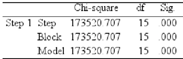
The set of output under the heading of Block 0: Beginning Block (Table A.6) describes the baseline model – that is a model that do not contains our explanatory variables and is only predicting with the intercept which SPSS denotes as constant. In Classification Table (Table A.6) we purely have the information of occurrences vs predictions of each category and the events most often verified. We can see that Not Defaulted Loans (𝑙𝑜𝑎𝑛_𝑠𝑡𝑎𝑡𝑢𝑠 = 0) appeared 279.914 times vs 58,995 of Defaulted loans (𝑙𝑜𝑎𝑛_𝑠𝑡𝑎𝑡𝑢𝑠 = 1) and its predictions were 100% for non-defaulted loans, which in overall, suggests that the model is correct 82.6% of the time. Variables in the Equation (Table A.7) shows us that the prediction of the model with only a constant, is significant (p-value<0.05). However, it is right roughly 83% of the time. Focusing on Block 1 model (Table A.8), the Omnibus Tests of Model Coefficients is used to check that the new model that contains the explanatory variables added is better than the baseline model that only considers the intercept. Chi-square testes are computed to check if there’s a significant difference between the Log-Likelihoods (-2LL) of the baseline model and the new model. Under Model Summary (Table A.9) it is possible to verify that -2 Log likelihood statistic is 139,825.39 and although Block 0 output does not give us the -2LL, we know that its value would be 313,346.09711_{. If the new model has a significantly reduced -2LL compared to the}

baseline, as in our case, then it suggests that the new model is explaining more of the variance in the outcome and is an improvement. It is also notable how significant the chi-squares are (p<0.05), so our new model is significantly better.

The Cox & Snell 𝑅2 _{value (0.401) tell us approximately how much variation in the}

outcome is explained by the model. Nagelkerke’s 𝑅2 _{suggests that the model}

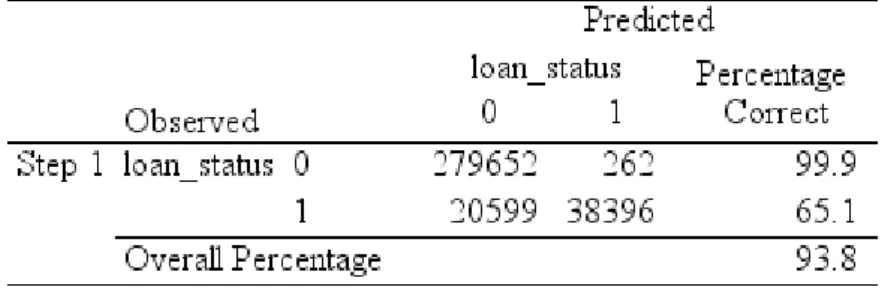
explains roughly 67% of the variation in the outcome. Moving to Classification

Table (Table A.10), the most important measure is Overall Percentage that

compares the observed vs predicted loan_status. We can see that the model is correctly classifying the outcome for 93.8% of the cases compared to 83% in the null model (intercept). The last Table (A.11) Variables in the Equation, already

24

has our explanatory variables, including the constant, and it gives us the weight (𝛽𝑖) that each variable has in the model and their explanatory power (p<0.05).

Considering the significant variables, the regression equation of the estimated model can be written as:

Z = −4.852 + 0.694𝑡𝑒𝑟𝑚 + 8.097𝑖𝑛𝑡_𝑟𝑎𝑡𝑒 + 0.016𝑑𝑡𝑖 + 0.111𝑖𝑛𝑞_𝑙𝑎𝑠𝑡_6𝑚𝑡ℎ𝑠 − 0.001𝑚𝑡ℎ𝑠_𝑠𝑖𝑛𝑐𝑒_𝑙𝑎𝑠𝑡_𝑑𝑒𝑙𝑖𝑛𝑞_1 + 0.107𝑝𝑢𝑏_𝑟𝑒𝑐 + 0.097𝑟𝑒𝑣𝑜𝑙_𝑢𝑡𝑖𝑙 − 0.025𝑡𝑜𝑡𝑎𝑙_𝑎𝑐𝑐 + 0.018𝑡𝑜𝑡𝑎𝑙_𝑟𝑒𝑐_𝑙𝑎𝑡𝑒_𝑓𝑒𝑒 + 6.989𝑐𝑜𝑙𝑙𝑒𝑐𝑡𝑖𝑜𝑛_𝑟𝑒𝑐𝑜𝑣𝑒𝑟𝑦_𝑓𝑒𝑒 + 0.005𝑚𝑡ℎ𝑠_𝑠𝑖𝑛𝑐𝑒_𝑙𝑎𝑠𝑡_𝑟𝑒𝑐𝑜𝑟𝑑_1 + 0.003𝑝𝑐𝑡_𝑡𝑙_𝑛𝑣𝑟_𝑑𝑙𝑞 + 0.031𝑜𝑝𝑒𝑛_𝑎𝑐𝑐 + 0.0396𝑎𝑐𝑐_𝑜𝑝𝑒𝑛_𝑝𝑎𝑠𝑡_24𝑚𝑡ℎ𝑠 + 0.227𝑑𝑖𝑠𝑏𝑢𝑟𝑠𝑒𝑚𝑒𝑛𝑡_𝑚𝑒𝑡ℎ𝑜𝑑

Although all variables included in the regression present explanatory power, the difference in their weight is obvious. There are two variables (int_rate and collection_recovery_fee) that have significantly larger 𝛽 and in contrast, the remaining variables seem to have residual load in the model. Having this in consideration and by the principle of parsimony12_{, a model with less variables}

could be considered. In that sense a regression equation for an additional model (Model 2), can be expressed as:

𝑍 = −4.852 + 8.097𝑖𝑛𝑡_𝑟𝑎𝑡𝑒 + 6.989𝑐𝑜𝑙𝑙𝑒𝑐𝑡𝑖𝑜𝑛_𝑟𝑒𝑐𝑜𝑣𝑒𝑟𝑦_𝑓𝑒𝑒

In the following sections only the results for Model 1 are going to be presented and in Table II, it is possible to see the comparisons between the two models and criteria for selection.

5.2

Model Validation

The results of bootstrap are shown in Table A.12. It is possible to see the estimate 𝛽 for every variable, and to interpret them, we check the example of dti.

12 _{Parsimonious means the simplest model/theory with the least assumptions and variables but}

25

It is observed that per year increase in term, increases the log odds of default by 0.023. We can also see that this result is very significant looking at its 𝑝 − 𝑣𝑎𝑙𝑢𝑒 = 0.001. The 95% confidence interval for the odds ratio of the effect of term is (0.013-0.032) suggesting that the odds of default increased about 1.3% to 3.2%. It is important to remark the differences of significance of the explanatory variables between our estimated model and bootstrapping, e.g. pub_rec appears not to have statistical power. Such differences are explained by the principle of

optimism, (Picard & Cook, 1984). Because of the maximum-likelihood technique

used to estimate the 𝛽_𝑖 of the variables, the logistic regression equation computes the best possible event predictions on the sample used to fit the model, that when applied to a different sample it outperforms.

Because of this effect, Giancristofaro & Salmaso (2003) state that is not enough to evaluate how well a regression equation predicts on a sample, and for that a goodness-of-fit analysis is not enough. It is necessary to obtain some quantitative and objective measures to determine if the model is restricted to scientific utility, if it determined to be sample-specific, or if it has predictive power.

5.3

Accuracy

Looking at the output (Table A.13) the first table to analyze is Group Statistics, in which it is shown a descriptive analysis of the means and standard deviation of the two groups (positive and negative), and in the last square, the total of the groups combined. Test Equality of Group Means (Table A.13) indicates if the

Loans in Default group or Loans in No Default Group were significantly different

in each of the predictive variables. In column Sig. we can derive the statistical significance of the group means for each of the explanatory variables. It is possible to determine that among the variables included in the model the two groups are significantly different. That result gives us the idea that the predictive variables seem to be discriminant. Summary of Canonical Discriminant Function derives how strong is the relationship between the predictor variables and the outcome that we are trying to predict. In Eigenvalues table (Table A.15) we can square the canonical correlation and interpret it as a magnitude (equivalent to 𝑅2

26

Wilk’s Lambda (Table A.16) gives us the idea of the statistical significance of

prediction model, or in other words, if the predictive variables predict the outcome at a significant statistical level. Interpreting the Sig. column, it is possible to determine that all predictors are statistically significant once that 𝑝 − 𝑣𝑎𝑙𝑢𝑒 < 0.05. Standardized Canonical Coefficients (Table A.17) reveal that the variable that has the highest weight in the prediction of group membership is

collection_recovery_fee (0.865), that is a consistent result according to the

following table Structure Matrix (Table A.18). Classification Results table (Table A.19) measures the accuracy of the predictive model vs observed (actual) results. We verify that the predicted No Default Loans correspond to 99.8% of the observed and that the predicted Default Loans, correspond to 34.2% of the observed. All in all, using the variables of the estimated model it is fair to say that it is a significant model when it comes to predict group membership.

From classification results table we can derive sensitivity and specificity:

𝑆𝑒𝑛𝑠𝑖𝑡𝑖𝑣𝑖𝑡𝑦 = 279.375

279.375 + 539= 0.998 𝑆𝑝𝑒𝑐𝑖𝑓𝑖𝑐𝑖𝑡𝑦 = 20.154

38.841 + 20.154 = 0.342

With these two measures, it is possible to plot the resulting ROC curve (Figure A.4). We can confirm that the curve is very-well shaped for our purposes, and that the AUC is 90.4% (Table A.20). Given the results, it is fair to say that the estimated model has a high discriminant power.

5.4

Calibration

Table A.25 shows that 𝑝 − 𝑣𝑎𝑙𝑢𝑒 < 0.05, meaning that we reject the null hypothesis of a good fit. Although the model seems to poor in terms of calibration, its power is much influenced by the sample size, like other chi-square tests (Yu, Xu, & Zhu, 2017), especially when datasets are large (over 25k). Given the proposition, the same test was applied to a shorter sample (1,000 subjects) from

27

original dataset, and as verified in Table A.22, Hosmer and Lemeshow test seems to be insignificant (𝑝 − 𝑣𝑎𝑙𝑢𝑒 > 0.05), which means that we accept the null and the model demonstrates good calibration.

It is also important to remind that a predictive model cannot have both a perfect calibration and a perfect accuracy (Diamond, 1992), there is always a trade-off between the two dimensions, meaning that a model that presents a maximization of accuracy will be weaker in calibration, although is it desirable an equilibrium between the two.

All in all, it is more important to have a good accuracy level once that the model can be recalibrated without sacrificing accuracy, (Harrell et al., 1996).

5.5

Model Comparison

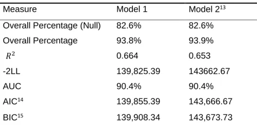
Table 2 - Model Comparison

Measure Model 1 Model 213

Overall Percentage (Null) 82.6% 82.6%

Overall Percentage 93.8% 93.9% ‘𝑅2 _{0.664 0.653} -2LL 139,825.39 143662.67 AUC 90.4% 90.4% AIC14 _{139,855.39 143,666.67} BIC15 _{139,908.34 143,673.73}

From the Table II, it is possible to see that Model 1 and Model 2 seem to be equivalent when adding the explanatory variables. In terms of accuracy, both

13 _{Results of the output in the Annex, Tables A.26, A.27, A.28, A.30 and Table A.29.}

14 _{Akaike information criterion - (AIC) (Akaike, 1974) is a fined technique based on in-sample fit}

to estimate the likelihood of a model to predict/estimate the future values, used to perform model comparisons. AIC is calculated through −2𝐿𝐿 + 2 ∗ #𝑝𝑟𝑒𝑑𝑖𝑐𝑡𝑜𝑟𝑠, and according to it. A lower AIC value indicates a better fit.

15 _{Bayesian information criterion - (BIC) is another criterion for model selection that measures}

the trade-off between model fit and complexity of the model. 𝐵𝐼𝐶 = −2𝐿𝐿 + log(𝑛) ∗ #𝑝𝑟𝑒𝑑𝑖𝑐𝑡𝑜𝑟𝑠. A lower BIC value indicates a better fit.

28

models stand at a good level and the downgrade of complexity seems to be higher than the loss on AUC. Despite the parallel results in terms of accuracy and calibration, Model 1 presents lower AIC and BIC than Model 2.

6.

Application to a loan portfolio

Model comparison can be a quite hard decision and once that we are modelling a probability of default, the model is going to be tested for a specific threshold that provides for higher profits. For this purpose, the method of

backtesting was used. Backtesting offers the best opportunity for incorporating

suitable incentives into the internal model’s approach in a manner that is consistent and that will cover a variety of circumstances (Banking & Supervision, 1996). This method has three objectives:

• Determine whether the assessments have come close enough to the verified outputs, in order to determine that such assessments are statistically compatible with the relevant outputs.

• Aid risk managers when diagnosing problems, within their risk models, as well as to improve them.

• Rank the performances of several alternative risk models, in order to determine which model provides the best performance assessment. To perform the test, there were some measures that had to be considered as the interest rate, loss given default (LGD), funding costs for the Financial Institution and a management cost. The interest rate was calculated through weighted average and the rate is 12.25%. Loss given default was assumed to be 0.5 (in this case the LGD is dependent on country or state legal conditions, on the type of asset recovery and on credit management processes, thus it will be a relevant variable per each FI). Funding costs were set at the average of the Daily Treasury Yield Curve Rates16 _{at 3 and 5 years, once that the terms of the loans}

for 36 or 60 months. The two rates were 1.43% and 1.40% and the average is

16 _{U.S Departement of the Treasury. Daily Treasury Yield Curve Rates. Available from:}

29

1.415%. The management costs were assumed to be 1%. Given the above measures, the cut-off for probability of default is 0.175217_{. Table III summarizes}

the profitability obtained by each model.

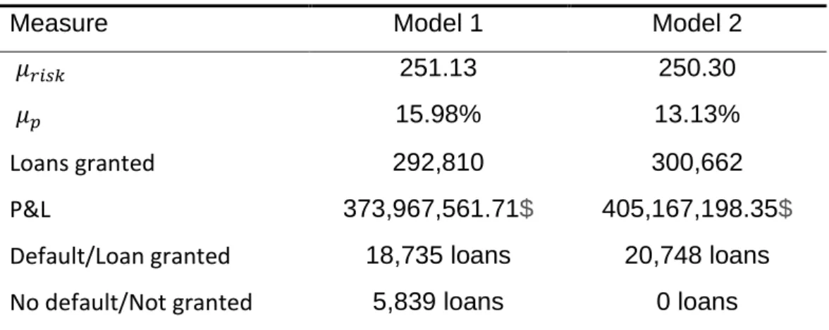
Table 3 - Financial measures of each model

Measure Model 1 Model 2

‘𝜇𝑟𝑖𝑠𝑘 251.13 250.30

‘𝜇𝑝 15.98% 13.13%

Loans granted 292,810 300,662

P&L 373,967,561.71$ 405,167,198.35$

Default/Loan granted 18,735 loans 20,748 loans No default/Not granted 5,839 loans 0 loans

Looking at the table it is possible to see that Model 2 presents lower risk than Model 1. The mean value of risk is lower in Model 2 and the probability for default as well. In terms of loans granted, Model 2 is higher than Model 1 in 7,852 loans and therefore the profitability obtained with Model 2 is higher in 31,199,636.64$ than Model 1.

To measure accuracy of risk management tools, Default/Loan granted (false positive) and No default/Not granted (false negative) were computed. They are translated in the potential costs that the company might incur and the missing business opportunities, respectively. Relatively to the costs in case of default,

Model 2 appears to drive comparatively higher costs, in the counterpart, Model 2

does not present missing business opportunity. Given the values obtained, it is fair to say that Model 2 took advantage of false “red flags” in 5,839 loans, that should compensate for the potential costs to incur in 2,013 loans.

Furthermore, to obtain a projection of the current loans that are still ongoing, extracted from the original database18_{, Model 2, was applied and the}

profit expected at the end of one year is 222,169,550.15$.

17 _{(interest rate-funding costs-management costs)/ (1+interest rate)/LGD}

= (0.1225-0.01415-0.01) / (1+0.1225)/0.5 = 0.1752.

30

7.

Conclusions

The objective of this study was to model the probability of default of an American loan portfolio. To achieve it, the logit model was used in order to understand the factors that have more weight on a possible default event and construct the regression equation that calculates the risk of every operation.

From there it was possible to determine a cut-off value for the probability of default and assess the impact in the P&L through Backtesting.

The two models present equivalence in terms of discriminatory and calibration power, for that reason, the model choice can be based on the profitability that each of the models could suppose.

In the end, using Model 2 could benefit the lender because it accounted for +31,199,636.64$ than Model 1.

Limitations of this work cling on the type of business database. Once we only have access to the crude database, it was difficult to identify the variables that could be part of this consumer credit model. Once they are very different and have broad sense, they can be part of different credit models, as mortgage or auto, for instance.

All in all, the results given by the statistical tests seem very consistent, and good measures of model validation, calibration and accuracy were obtained, which suggests that the variables chosen are a good combination to model the probability of default.

As a suggestion for future research, it could be beneficial the accuracy of the various credit systems that are present in the database and model each one of them separately, to obtain more consistent and applicable results.

8.

Bibliography

Altman, E. I. (1968). Financial Ratios, Discriminant Analysis and the Prediction of Corporate Bankruptcy. The Journal of Finance, 589–609.

Altman, E. I. (1988). Default Risk, Mortality Rates and Performance of Corporate Bonds.

31

Altman, E. I. (1989). Measuring Corporate Bond Mortality and Performance.

The Journal of Finance, 44(4), 909–922.

Altman, E. I. (1994). Corporate Distress Diagnosis: Comparisons using linear discriminant analysis and neural networks (the Italian experience). Journal

of Banking and Finance, 505–529.

Altman, E. I. (2005). An Emerging Market Credit Scoring System for Corporate Bonds. Emerging Markets Review, 6(4), 311–323.

Altman, E. I., Haldeman, R. G., & Narayanan, P. (1977). ZETA Analysis - A New Model to Identify Bankruptcy Risk of Corporations. Journal of Banking

and Finance, 1(1), 29–54.

Altman, E. I., & Narayanan, P. (1997). An International Survey of Business Failure Classification Models. Financial Markets, Institutions and

Instruments, 6(2), 1–57.

Altman, E. I., & Saunders, A. (1998). Credit risk measurement : Developments over the last 20 years. Journal of Banking and Finance, 21, 1721–1742. Asquith, P., Mullins, D. W., & Wolff, E. D. (1989). Original Issue High Yield

Bonds: Aging Analyses of Defaults, Exchanges, and Calls. The Journal of

Finance, 44(4), 923–952.

Banking, B. C. on, & Supervision. (1996). Supervisory Framework for the use of “Backtesting” in Conjuction with the Internal Models Approach to Market Risk Capital Requirements.

Berkson, J. (1944). Application of the Logistic Function to Bio-Assay. Journal of

the American Statistical Association, 39(227), 357–365.

Bliss, C. I. (1935). The Calculation of the Dosage‐Mortality Curve. Annals of

Applied Biology, 22(1), 134–167.

Bouteillé, S., & Coogan-Pushner, D. (2013). The Handbook of Credit Risk

Management: Originating, Assessing, and Managing Credit Exposures.

John Wiley & Sons, Inc.

Chambers, E. A., & Cox, D. R. (1967). Accuracy between alternative binary response models. Biometrika, 54(3), 573–578.

Coats, P. k., & Fant, L. F. (1993). Recognizing Financial Distress Patterns Using a Neural Network Tool. Financial Management Association

32

International, 142–155.

Cramer, J. S. (2003). Logit Models from Economics and other Fields. Cambridge University Press.

Diamond, G. A. (1992). What price perfection? Calibration and accuracy of clinical prediction models. Journal of Clinical Epidemiology, 45(1), 85–89. Durand, D. (1941). Risk Elements in Consumer Instalment Financing. National

Bureau of Economic Research, 237.

Giancristofaro, R. A., & Salmaso, L. (2003). Model Performance Analysis and Model Validation in Logistic Regression. Statistica, 63(2), 375–396. Hand, D. J., & Henley, W. E. (1997). Statistical Classification Methods in

Consumer Credit Scoring: A Review. Journal of the Royal Statistical

Society, 160(3), 523–541.

Hao, C., Alam, M. M., & Carling, K. (2010). Review of the Literature on Credit Risk Modeling: development of the past 10 years. Banks and Bank

Systems, 43–60.

Harrell, F. E., Lee, K. L., & Mark, D. B. (1996). Multivariable Prognostic Models: Issues in developing models, evaluating assumptions and adequacy, and measuring and reducing errors. Statistics in Medicine, 5, 361–387.

Hosmer, D. W., & Lemeshow, S. (1980). Communications in Statistics - Theory and Methods Goodness of fit tests for the multiple logistic regression model. Communications in Statistics - Theory and Methods, 1043–1069. Hosmer, D. W., & Lemeshow, S. (2000). Applied Logistic Regression.pdf

(Second Edi). New York: John Wiley & Sons, Inc.

Jacobson, T., & Roszbach, K. (2003). Bank Lending Policy, Credit Scoring and Value-at-Risk. Journal of Banking and Finance, 27, 615–633.

Jonkhart, M. J. L. (1979). On the term structure of interest rates and the risk of default. An analytical approach. Journal of Banking and Finance, 3(3), 253– 262.

Kealhofer, S. (1997). Portfolio Management of Default Risk. KMV Corporation. San Francisco.

Lin, S. L. (2009). A new two-stage hybrid approach of credit risk in banking industry. Expert Systems with Applications, 36(4), 8333–8341.

33

Luppi, B., Marzo, M., & Scorcu, A. E. (2008). Credit risk and Basel II: Are

nonprofit firms financially different? Rimini Centre for Economic Analysis

(Vol. 4).

Niu, J. (2004). Managing Risks in Consumer Credit Industry.

Picard, R. R., & Cook, R. D. (1984). Cross-validation of Regression Models.

Journal of the American Statistical Association, 79(387), 575–583.

Platt, H. D., & Platt, M. B. (1991). A note on the use of industry-relative ratios in bankruptcy prediction. Journal of Banking and Finance, 15(6), 1183–1194. Saunders, A., & Allen, L. (2002). Credit Risk Measurement: New Approaches to

Value at Risk and Other Paradigms (Second Edi). New York: John Wiley &

Sons, Inc.

Scott, J. (1981). A Comparison of Empirical Predictions and Theoretical Models.

Journal of Banking and Finance, 5, 317–344.

Siddiqi, N. (2006). Credit Risk Scorecards - Developing and Implementing

Intelligent Credit Scoring. Hoboken, New Jersey: John Wiley & Sons, Inc.

Somerville, R. A., & Taffler, R. J. (1995). Banker Judgement versus Formal Forecasting Models: The Case of Country Risk Assessment, 19, 281–297. Supervision, B. C. on B. (2000). Range of Practice in Bank’s Internal Ratings

Systems.

Tibshirani, R., James, G., Witten, D., & Hastie, T. (2013). Introduction to

Statistics Using R. Synthesis Lectures on Mathematics and Statistics (Vol.

11). New York: Springer.

Trippi, R. R., & Turban, E. (1997). Neural networks in finance and investing. Using artificial intelligence to improve realworld performance. Journal of

Forecasting, 13(Revised ed. Irwin, Homewood, IL.), 144–146.

Turkman, M. A. A., & Silva, G. L. (2000). Modelos Lineares Generalizados - Da

Teoria à Prática.

Walter, S. Basel II and Revisions to the Capital Requirements Directive -Key elements of the BCBS reform programme - Remarks by Stefan Walter (Secretary General, BCBS). (2010).

West, R. C. (1985). A factor-analytic approach to bank condition, 9(January 1984), 253–266.

34

Yu, W., Xu, W., & Zhu, L. (2017). A modified Hosmer–Lemeshow test for large data sets. Communications in Statistics - Theory and Methods, 46(23), 11813–11825.

Trading Economics (2019). United States Consumer Credit Change. Available from: https://tradingeconomics.com/united-states/consumer-credit

[Accessed: 15/09/2019].

BIS (2019). About the BCBS. History of the Basel Committee. Available from: https://www.bis.org/bcbs/history.htm [Accessed: 3/08/2019].

The LendingClub. Lending Club Loan Data. Available from:

https://www.kaggle.com/wendykan/lending-club-loan-data [Accessed: 15/04/2019].

U.S Departement of the Treasury. Daily Treasury Yield Curve Rates. Available from:https://www.treasury.gov/resource-center/data-chart-center/interest-rates/Pages/TextView.aspx?data=yieldYear&year=2019 [Accessed: 10/10/2019].

9.

Annex

35

Figure A.2 - Forecast for consumer credit market in the US

36 Table A.4 - Descriptive Analysis of Data

Table A.5 - Replacement of missing values of variable mths_since_last_delinq

37

Table A.8 - Multicollinearity for variable loan_status (VIF) Table A.7 - T-Test Paired Sample

38 Table A.9 - Model 1 Block 0 (Baseline model)

Table A.10 - Model 1 Variables in Equation

Table A.11 - Model 1 Omnibus test of model coefficients

39 Table A.13 - Model 1 Classification Table

40 Table A.15 - Model 1 Bootstrap

41 Table A.16 - Model 1 Group Statistics

42

Table A.17 - Model 1 Test Equality of Group Means

Table A.18 - Model 1 Eigenvalues

43

Table A.20 - Model 1 Standardized Canonical Discriminant Function Coefficients

44 Table A.21 - Model 1 Structure Matrix

45 Figure A.4 - Model 1 ROC Curve

Table A.23 - Model 1 AUC

Table A.24 - Model 1 Hosmer and Lemeshow Test for 338.909 subjects and 1.000 subjects

46 Table A.25 - Model 2 Block 0 (Baseline model)

Table A.26 - Model 2 Classification Table

47 Figure A.5 - Model 2 ROC Curve

48