D
D
e
e
t
t
e
e
r
r
m
m
i
i
n
n
a
a
n
n
t
t
s
s
o
o
f
f
t
t
h
h
e
e
p
p
o
o
r
r
t
t
u
u
g
g
u
u
e
e
s
s
e
e
g
g
o
o
v
v
e
e
r
r
n
n
m
m
e
e
n
n
t
t
b
b
o
o
n
n
d
d
y
y
i
i
e
e
l
l
d
d
s
s
ANDRÉ PINHO
RICARDO BARRADAS
M
M
a
a
r
r
ç
ç
o
o
2
2
0
0
1
1
8
8
W
WP
P
n
n.
.
º
º
2
20
01
18
8/
/0
03
3
DOCUMENTO DE TRABALHO WORKING PAPERD
D
e
e
t
t
e
e
r
r
m
m
i
i
n
n
a
a
n
n
t
t
s
s
o
o
f
f
t
t
h
h
e
e
p
p
o
o
r
r
t
t
u
u
g
g
u
u
e
e
s
s
e
e
g
g
o
o
v
v
e
e
r
r
n
n
m
m
e
e
n
n
t
t
b
b
o
o
n
n
d
d
y
y
i
i
e
e
l
l
d
d
s
s
11 ANDRÉ PINHO2 RICARDO BARRADAS3,4WP n. º 2018/03
DOI: 10.15847/dinamiacet-iul.wp.2018.03 1. Introduction ... 3 2. Literature review ... 43. Models and hypotheses ... 9
4. Data and econometric methodology ... 11
5. Results and discussion... 15
6. Conclusion ... 24
7. References ... 26
8. Appendix ... 30
1 The authors thank the helpful comments and suggestions of Diptes Bhimjee and Emanuel Leão. The
usual disclaimer applies.
2 Instituto Universitário de Lisboa (ISCTE-IUL), Lisboa, Portugal. Caixa Económica Montepio Geral, Lisboa,
Portugal. E-mail: andremcpinho@gmail.com
3 Instituto Universitário de Lisboa (ISCTE-IUL), Dinâmia’CET-IUL, Lisboa, Portugal. ESCS - Escola Superior
de Comunicação Social and ISCAL - Instituto Superior de Contabilidade e Administração de Lisboa, Instituto Politécnico de Lisboa, Lisboa, Portugal. E-mail: ricardo_barradas@iscte-iul.pt
D
D
e
e
t
t
e
e
r
r
m
m
i
i
n
n
a
a
n
n
t
t
s
s
o
o
f
f
t
t
h
h
e
e
p
p
o
o
r
r
t
t
u
u
g
g
u
u
e
e
s
s
e
e
g
g
o
o
v
v
e
e
r
r
n
n
m
m
e
e
n
n
t
t
b
b
o
o
n
n
d
d
y
y
i
i
e
e
l
l
d
d
s
s
ABSTRACT
This paper conducts an empirical examination of the determinants of the ten-, five- and one-year Portuguese government bond yields by performing a time series econometric analysis for the period between the first quarter of 2000 and the last quarter of 2016. The literature suggests that the evolution of government bond yields depends on three main risk drivers, namely credit risk, global risk aversion and liquidity risk. We estimate three equations for the ten-, five- and one-year Portuguese government bond yields, including eight independent variables (macroeconomic performance, fiscal conditions, foreign borrowing, the inflation rate, labour productivity, the demographic situation, global risk aversion and liquidity risk) to take into account all three risk drivers referred to in the literature. Our results show that there are no significant differences in the determinants of the Portuguese government bond yields among the different maturities, either in the long term or in the short term. Our results also confirm that all three of the risk drivers have exerted a strong influence on the evolution of the Portuguese government bond yields. Liquidity risk, the inflation rate and foreign borrowing are the main triggers of the rise in the Portuguese government bond yields, which does not counterweigh the beneficial effects played by the fiscal conditions, demographic situation and labour productivity.
KEYWORDS
Government Bond Yields, Long-term and Short-term Determinants, Credit Risk, Global Risk Aversion, Liquidity Risk, Portugal, ARDL Model
JEL CLASSIFICATION
1. INTRODUCTION
It is widely acknowledged that understanding the determinants that are responsible for the evolution of government bond yields over time assumes huge importance, not only for policy makers and their policies and budgetary decisions but also for investors and their potential returns and/or losses from their investment portfolios that include government bonds.
Accordingly, from a theoretical point of view, the evolution of government bond yields typically depends on the three main risk drivers, namely credit risk, global risk aversion and liquidity risk (Manganelli and Wolswijk, 2009; Arghyrou and Kontonikas, 2012; Afonso et al., 2015). Credit risk measures the risk of partial or total default of a sovereign borrower and typically is assessed through six different factors (Ichiue and Shimizu, 2012), specifically macroeconomic performance, fiscal conditions, foreign borrowing, the inflation rate, labour productivity and the demographic situation (ageing population). Global risk aversion measures the risk appetite and the level of financial risk perceived by investors. Liquidity risk measures the size and depth of the market, capturing the possibility of capital losses in the event of early liquidation or significant price changes due to a small number of transactions in the market. From an empirical point of view, the determinants of government bond yields are assessed by several econometric studies (Ardagna et al., 2007; Haugh et al., 2009; Laubach, 2009; Kumar and Baldacci, 2010; Ichiue and Shimizu, 2012; Dell’Erba and Sola, 2013; Pham, 2014; Poghosyan, 2014; Hsing, 2015).
This paper aims to assess the determinants of the ten-, five- and one-year Portuguese government bond yields by performing a time series econometric analysis for the period between the first quarter of 2000 and the last quarter of 2016. It introduces four important novelties to the existing literature. Firstly, the analysis is performed specifically for the Portuguese case, in a context in which the majority of empirical studies concerning this issue conduct panel data econometric analysis for a large set of countries as a whole. Note that the estimates produced by panel data econometric studies correspond to an average effect for a set of countries, ignoring the historical, social and economic country-specific circumstances. This paper tries to overcome this drawback by using time series data for Portugal. Portugal is an interesting case study, because it belongs to the euro area and recently suffered a financial and economic crisis that involved a request for international financial assistance due to the strong increase in the government bond yields and the corresponding worsening funding conditions in the bond markets. Secondly, the analysis covers the period before, during and after the crisis, whilst the existing empirical literature typically focuses on the period prior to the crisis. Hsing (2015) is the only exception, but this author’s analysis only focuses on the Spanish case.
Thirdly, the analysis incorporates all the risk drivers of government bond yields identified in the literature, which mitigates the problem of omitting relevant variables that could originate inconsistent and unbiased estimates (Wooldridge, 2003; Kutner et al., 2005; Brooks, 2009). Fourthly, the analysis contemplates the determinants of the ten-, five- and one-year Portuguese government bond yields, which is a novelty to the literature.
Against this backdrop, we build and estimate three equations for the ten-, five- and one-year Portuguese government bond yields, respectively, using eight independent variables to take into account all three risk drivers referred to in the literature (macroeconomic performance, fiscal conditions, foreign borrowing, the inflation rate, labour productivity, the demographic situation, global risk aversion and liquidity risk). The estimates are produced through the autoregressive distributed lag (ARDL) estimator due to the existence of a mixture of variables that are stationary in levels and stationary in first differences.
The paper concludes that there are no significant differences regarding the determinants of the Portuguese government bond yields among the different maturities considered, either in the long term or in the short term. It also confirms that all of three of the risk drivers have exerted a strong influence on the evolution of the Portuguese government bond yields. Liquidity risk, the inflation rate and foreign borrowing are the main triggers of the rise in the Portuguese government bond yields, which does not counterweigh the beneficial effects played by fiscal conditions, the demographic situation and labour productivity.
The paper is organised as follows. Section 2 presents a literature review on the main determinants of government bond yields. In Section 3, we construct three equations to describe the behaviour of the ten-, five- and one-year Portuguese government bond yields and present the expected theoretical effects of each variable on these yields. The data and econometric methodology are described in Section 4. The empirical results are discussed in Section 5. Finally, Section 6 concludes.
2. LITERATURE REVIEW
The existing literature related to the determinants of government bond yields or sovereign bond yields,5 either single-country or panel data studies, typically models government bond yields by considering three different main risk drivers (Manganelli and Wolswijk, 2009; Arghyrou and
5 Government bond yields and sovereign bond yields are normally used interchangeably. Henceforth, we
Kontonikas, 2012; Afonso et al., 2015): credit risk, global risk aversion and liquidity risk (Figure 1).
Figure 1 – Drivers of government bond yields
Government Bond Yields
Credit Risk Macroeconomic Performance Fiscal Conditions Foreign Borrowing Inflation Rate Labour Productivity
Demographic Situation (Ageing) Global Risk Aversion
Liquidity Risk
Source: Authors’ representation based on Manganelli and Wolswijk (2009), Arghyrou and Kontonikas (2012) and Afonso et al., 2015
Credit risk aims to capture the risk (i.e. the probability) of partial or total default of a sovereign borrower, which happens when a certain government does not fulfil its financial obligations in a timely manner. This type of risk depends essentially on six dimensions, namely macroeconomic performance, fiscal conditions, foreign borrowing, the inflation rate, labour productivity and the demographic situation (ageing population) of a particular country (Ichiue and Shimizu, 2012).
Macroeconomic performance tends to be assessed using the potential growth of the gross domestic product (Pham, 2014; Poghosyan, 2014) or the growth rate of the gross domestic product (Kumar and Baldacci, 2010; Hsing, 2015). According to Laubach (2009) and Poghosyan (2014), the linkage between macroeconomic performance and government bond yields can be explained using Euler’s equation concerning consumers’ utility maximisation problem. Effectively, following the Ramsey model of economic growth with representative household preferences described by the constant elasticity of substitution utility function and a production process described by the Cobb–Douglas function, there is a positive relationship between output growth and government bond yields, either in a closed economy or in an open economy. In addition, a better macroeconomic performance usually leads to lower levels of unemployment, in line with the predictions of Okun’s law, and higher wages, which favour a rise in the inflation rate following the Phillips curve and therefore a rise in government bond yields. On the other hand, Poghosyan (2014) suggests that positive deviations of the output growth from its potential level may reduce government bond yields, as the country’s temporary taxing capacity increases. This rationale could also apply to negative deviations of the output growth from its potential level, which decrease the country’s taxing capacity, causing a rise in government bond yields. Cantor and Packer (1996) stress that a higher rate of economic growth suggests that a country’s existing debt burden will become easier to service over time,
As regards fiscal conditions, the government debt and primary balance (Kumar and Baldacci, 2010; Ichiue and Shimizu, 2012; Pham, 2014; Poghosyan, 2014) or even the budget balance and current account balance (Afonso and Rault, 2011) are the variables that more often appear as determinants of government bond yields. The literature presents two different channels through which fiscal conditions may influence interest rates positively: the crowding-out effect and the default risk premium. Through the crowding-crowding-out effect, private investment may be crowded out by fiscal expansion, which results in a smaller steady-state capital stock, leading to a higher marginal product of capital and thus an increase in the level of interest rates (Engen and Hubbard, 2004). According to the default risk premium, the deterioration of fiscal conditions leads to a higher probability of default and consequently a demand for a higher risk premium by investors, which in turn raises government bond yields (Kumar and Baldacci, 2010). The literature also presents some interesting conclusions regarding fiscal conditions. Firstly, some empirical studies tend to use expected fiscal deficits rather than past or current fiscal deficits to measure the impact of fiscal conditions on long-term government bond yields (Haugh et al., 2009; Ichiue and Shimizu, 2012). Secondly, the impact of the level of public debt turns out to be lower quantitatively than that of fiscal deficits, contradicting the theoretical belief that stock fiscal variables (e.g. public debt) influence long-term interest rates but flow fiscal variables (e.g. fiscal deficit) do not (Engen and Hubbard, 2004). Note that the majority of empirical studies conclude that fiscal imbalances tend to raise long-term government bond yields in a context in which the impact ranges from 2 to 5 basis points for stock fiscal variables, such as the ratio between the public debt and the gross domestic product (Ardagna et al., 2007; Poghosyan, 2014), and from 10 to 25 basis points if flow fiscal variables, such as fiscal deficits (Laubach, 2009) or primary balances (Ardagna et al., 2007), are considered. This probably happens because flow variables provide useful information for forecasting future stock variables, particularly when they are revealed to be persistent over time (Ichiue and Shimizu, 2012). Against this backdrop, Ardagna et al. (2007), using a panel of 16 OECD countries and historical data from 1960 to 2002, conclude that the effects on interest rates increase as a country’s debt grows and its fiscal balance becomes weaker. In addition, Kumar and Baldacci (2010) conclude that larger fiscal deficits and higher levels of public debt lead to a significant increase in interest rates in a context in which the magnitude of such impacts reflects the initial fiscal conditions as well as the institutional and structural conditions and spillovers from global financial markets. Dell’Erba and Sola (2013), using a sample of 17 OECD countries, point out that common fiscal shocks lead to adjustments in European government bond yields, having a greater impact in smaller and peripheral countries. This may suggest that bond owners tend to rearrange their investment portfolios by selling their debt securities issued by those countries
and reinvesting in government bonds of countries with stronger economies and better fiscal conditions.
Regarding foreign borrowing, the level of external debt tends to be the variable used as a proxy for this dimension (Cantor and Packer, 1996; Ichiue and Shimizu, 2012). Hence, Gros (2011) and Ichiue and Shimizu (2012) suggest that, when an increase in the public debt is financed entirely by borrowing from external sources, the increase in the interest rate is approximately twice the size that it would be if it were financed by domestic savings. The argument is that the losses tend to be greater when the government depends more on domestic investors and therefore there is a strong incentive to choose to increase the national tax revenues instead of declaring a default. Thus, a higher level of external debt is normally associated with a higher risk of default (Cantor and Packer, 1996).
Inflation, either through historical rates (Ardagna et al., 2007; Poghosyan, 2014) or through expected rates (Hsing, 2015), influences nominal interest rates through two different channels: the level of inflation rate by itself and the uncertainty that is normally associated with it. Accordingly, Kumar and Baldacci (2010) suggest that higher inflation expectations may push government bond yields upwards through the increase in the inflation premium embodied in nominal rates, especially at times when the output deviations are positive or there are concerns about the monetisation of debt. This happens because investors want to be compensated for the rising prices. Baldacci et al. (2008) emphasise that inflation expectations could also generate macroeconomic uncertainty, leading to a higher country risk premium and therefore a rise in government bond yields. This suggests that investors tend to associate higher rates of inflation with the existence of structural problems in the government’s finances and/or with a certain degree of political instability (Cantor and Packer, 1996). Hsing (2015), through a single-country analysis for Spain over the period from 1999 to 2014, concludes that an increase in the expected inflation rate contributes to an increase in Spanish government bond yields.
Labour productivity and the demographic situation are less commonly used in empirical studies on the determinants of government bond yields. In relation to labour productivity, Ichiue and Shimizu (2012) employ a forecast of the annualised labour productivity growth rate and conclude that an increase in the expected productivity growth rate leads to a rise in the level of interest rates to a similar extent. In fact, higher labour productivity enables corporations to afford higher wages, which in turn contribute to higher inflation and therefore to an increase in the risk premiums demanded by investors.
As regards the demographic situation, the literature presents contradictory effects on long-term interest rates (Ichiue and Shimizu, 2012). On the one hand, it is often argued that population ageing lowers the marginal productivity of capital and reduces the investment
demand through a decrease in the labour supply, which in turn contributes to a decline in interest rates. A reduction in the level of interest rates could also be explained by an increase in the demand for financial assets by elderly people, particularly for safer financial assets, like government bonds. On the other hand, it is often claimed that an ageing population can contribute to an increase in interest rates through the life cycle hypothesis, according to which individuals begin to spend their savings after retirement, which leads to a decrease in the savings rate and in the amount of assets held by retired people. An ageing population also motivates a rise in the level of interest rates through the expectations of greater deterioration of fiscal conditions caused by the corresponding decline in revenues from taxes and the concomitant increase in social security benefits. Nonetheless, Ichiue and Shimizu (2012) conclude that a strong positive relationship exists, finding that a decline in the working-age population ratio (a proxy for a higher level of population ageing) favours a decrease in the interest rates.
Global risk aversion aims to capture the risk appetite and the level of financial risk perceived by investors as well as their sentiment towards the market of government bonds. According to the majority of empirical studies, corporate bond spreads (Haugh et al., 2009) or stock market implied volatility indexes (Afonso et al., 2015) are used to measure global risk aversion. All of them find that this risk driver has a strong negative effect on government bond yields, mainly during periods of tightening financial conditions (Haugh et al., 2009).
Finally, liquidity risk refers to the size and depth of the government bond market and aims to capture the possibility of capital losses in the event of early liquidation or significant price changes resulting from a small number of transactions in the market. Most empirical studies around this issue tend to use government bond bid–ask spreads (Afonso et al., 2015) and/or the volume of transactions or the share of a country’s government debt in the total government debt of the euro area countries as a whole (Gómez-Puig, 2006; Attinasi et al., 2009; Haugh et al., 2009; Gerlach et al., 2010; Arghyrou and Kontonikas, 2012; Bernoth et al., 2012). Liquidity tends to vary inversely with the size of the market, as investors can trade quickly and face a lower risk that prices will change significantly in large bond markets; therefore, they demand less compensation in terms of the yield (Haugh et al., 2009). Moreover, liquidity effects are found to be greater during periods of tightening financial conditions and higher interest rates, during which the market players agree to trade lower yields for higher government debt liquidity (Favero et al., 2010).
This increasing amount of theoretical work on the determinants of government bond yields matches the emergence of some empirical studies regarding this issue (Ardagna et al., 2007; Haugh et al., 2009; Laubach, 2009; Kumar and Baldacci, 2010; Ichiue and Shimizu,
2012; Dell’Erba and Sola, 2013; Pham, 2014; Poghosyan, 2014; Hsing, 2015). Four characteristics are common to most of them. Firstly, the majority of them perform panel data econometric analysis by analysing the determinants of government bond yields in a large set of countries as a whole. Laubach (2009) and Hsing (2015) are the only exceptions, but their analyses are centred on the USA and Spain, respectively. Secondly, they only consider the pre-crisis period. The study by Hsing (2015) is the only one that takes into account the pre-crisis period in its estimates, but it only focuses on Spain. Thirdly, they only take into account some of the three risk drivers identified in the literature. This highlights the risk of potential inconsistent and unbiased estimates due to the problem of omitted relevant variables (Wooldridge, 2003; Kutner
et al., 2005; Brooks, 2009). Ichiue and Shimizu’s (2012) study is the only exception, but they
perform a panel data econometric analysis for ten developed countries (Australia, Canada, Germany, Japan, New Zealand, Norway, Sweden, Switzerland, the United Kingdom and the USA). Fourthly, all of them analyse the determinants of ten-year government bond yields.
This paper aims to conduct an empirical analysis of the determinants of government bond yields by performing a time series econometric analysis for Portugal over the period from the first quarter of 2000 to the last quarter of 2016. It aims to contribute to the existing literature in four different ways, namely by analysing Portugal; incorporating the pre-crisis, crisis and post-crisis periods, respectively; including the aforementioned three risk drivers of government bond yields; and assessing the determinants not only of ten-year government bond yields but also of five-year and one-year government bond yields, respectively.
3. MODELS AND HYPOTHESES
Our econometric models estimate three equations for the ten-, five- and one-year Portuguese government bond yields, respectively. They include eight independent variables taking into account the aforementioned three risk drivers of government bond yields: macroeconomic performance, fiscal conditions, foreign borrowing, the inflation rate, labour productivity, the demographic situation, global risk aversion and liquidity risk.
Our long-term equations for the Portuguese government bond yields take the following forms:
(1)
(2)
(3)
where
t
is the time period (quarters),GBY
10Y are the ten-year Portuguese government bond yields,GBY
5Y are the five-year Portuguese government bond yields,GBY
1Y are the one-year Portuguese government bond yields, MP is the macroeconomic performance,FC
are the fiscal conditions, FB is foreign borrowing, IR is the inflation rate, LP is labour productivity,DS
is the demographic situation (ageing population),GRA
is global risk aversion,LR
is liquidity risk and
is an independent and identically distributed (white noise) disturbance term with a null average and constant variance (homoscedastic).Regarding the effect of each independent variable on the government bond yields, the fiscal conditions, foreign borrowing, the inflation rate, labour productivity and liquidity risk are expected to exert a positive effect, whereas global risk aversion is expected to have a negative impact. Macroeconomic performance and the demographic situation have an undetermined effect on government bond yields. Thus, the coefficients of these variables are expected to have the following signs:
(4)
Macroeconomic performance has an ambiguous effect on government bond yields. On the one hand, a positive effect is expected according to the aforementioned Ramsey model of economic growth (Laubach, 2009; Poghosyan, 2014) and according to the expectations of lower levels of unemployment and higher levels of inflation explained by Okun’s law and the Phillips curve, respectively. On the other hand, a negative effect is anticipated due to the expectation that the debt will become easier to service over time in an environment of higher economic growth (Cantor and Packer, 1996; Poghosyan, 2014).
The fiscal conditions are also expected to exert a positive effect on government bond yields due to the abovementioned crowding-out effect and default risk premium (Engen and Hubbard, 2004; Kumar and Baldacci, 2010).
The effect of foreign borrowing on government bond yields is also positive, because investors tend to require a higher risk premium when the public debt is increasingly being
t t t t t t t t t Y t
MP
FC
FB
IR
LP
DS
GRA
LR
GBY
10
0
1
2
3
4
5
6
7
8
t t t t t t t t t Y tMP
FC
FB
IR
LP
DS
GRA
LR
GBY
5
0
1
2
3
4
5
6
7
8
t t t t t t t t t Y tMP
FC
FB
IR
LP
DS
GRA
LR
GBY
1
0
1
2
3
4
5
6
7
8
financed by external sources instead of domestic sources due to a greater incentive to declare default in that situation (Cantor and Packer, 1996; Gros, 2011; Ichiue and Shimizu, 2012).
The inflation rate affects government bond yields positively, because it is treated as a proxy for uncertainty and instability by investors, which leads to higher risk premiums and consequently to a rise in the level of interest rates (Cantor and Packer, 1996; Baldacci et al., 2008; Kumar and Baldacci, 2010).
Labour productivity is expected to exert a positive impact on government bond yields. The argument is that an increase in labour productivity contributes to a rise in wages, which feeds inflation expectations and consequently produces an increase in government bond yields.
The demographic situation (an ageing population) has an ambiguous effect on government bond yields (Ichiue and Shimizu, 2012). On the one hand, an ageing population lowers the marginal productivity of capital and reduces the investment demand through a decrease in the labour supply, which favours a decrease in government bond yields. On the other hand, an ageing population boosts the decrease in the savings rate and feeds expectations of greater deterioration of fiscal conditions, which favours an increase in government bond yields.
Government bond yields are affected negatively by global risk aversion, because in periods of greater risk aversion, investors tend to rearrange their portfolios to favour less risky assets (e.g. government bonds), which leads to a decrease in government bond yields (Haugh et
al., 2009; Afonso et al., 2015).
Liquidity risk also exerts a positive effect on government bond yields, because investors tend to require a higher risk premium for more risky assets (e.g. illiquid government bonds), boosting their level of interest rates (Haugh et al., 2009).
4. DATA AND ECONOMETRIC METHODOLOGY
Quarterly data were collected from the first quarter of 2000 to the last quarter of 2016, corresponding to the period and frequency for which data for the dependent and independent variables are available. Our sample therefore covers the period after the creation of the euro, which represents a change in the institutional context in which the Portuguese government bonds have evolved.
In relation to the definition of each variable and the corresponding sources, the Portuguese government bond yields (ten-, five- and one-year maturities) were collected from the
Bloomberg database. Since the available data were on a daily frequency, we computed the arithmetic average for each quarter of the respective government bond yields.
Macroeconomic performance is proxied by the annual percentage change (year-on-year) in the gross domestic product (at constant prices and in millions of euros), extracted from the Portuguese National Accounts, available at Instituto Nacional de Estatística.
The proxy for fiscal conditions is the total general government gross debt (at current prices and in millions of euros) as a percentage of the gross domestic product (at current prices and in millions of euros), obtained directly from the Bank of Portugal database.
We use the total net external debt (at current prices and in millions of euros) as a percentage of the gross domestic product (at current prices and in millions of euros) to measure foreign borrowing. This variable was extracted directly from the Bank of Portugal database.
The inflation rate used here is the annual percentage change (year-on-year) in the consumer price index, which was collected from the Bank of Portugal database. Note that we calculated the arithmetic average for each quarter of the respective annual percentage changes (year-on-year) taking into account the fact that this variable is only available on a monthly basis.
Labour productivity corresponds to the annual percentage change (year-on-year) in the gross domestic product (at current prices and in millions of euros) divided by the total employment (thousands of persons). Both variables were collected from the Portuguese National Accounts, available at Instituto Nacional de Estatística.
The demographic situation (ageing population) is weighted by the activity rate, which can be described as the total active population divided by the total population aged between 15 and 64 years.6 This variable was extracted directly from the Bank of Portugal database.
The proxy for global risk aversion corresponds to the natural logarithm of the S&P500 implied stock market volatility index (i.e. the so-called VIX index), which was collected from the Bloomberg database. We also calculated the arithmetic average for each quarter of the respective natural logarithms, because this variable is available on a daily basis.
Finally, the liquidity risk is measured using the importance of the Portuguese general government consolidated gross debt in the government consolidated gross debt of the euro area countries, which give us an indication of Portugal’s public debt market share within the euro area countries.7 Both variables are available from the Eurostat database.
6 Note than an increase in this variable means an increase in the active population, which indicates a less
ageing population.
7 It should be noted that an increase in this variable means that the Portuguese government bonds are
becoming more liquid; that is, they have lower liquidity risk. Thus, taking into account the aforementioned positive relationship between liquidity risk and government bond yields, we expect this variable to exert a negative effect on Portuguese government bond yields.
Figure
A1
to Figure A11 in the Appendix contain the plots of our dependent and independent variables.Table
A1
in the Appendix exhibits the descriptive statistics for each variable, and Table 1 shows the correlation coefficients between them.Table 1 – Correlation coefficients between the variables
GBY10Y MP FC FB IR LP DS GRA LR GBY10Y 1 MP -0.51*** 1 FC 0.18 -0.33*** 1 FB 0.13 -0.41*** 0.95*** 1 IR 0.36*** 0.13 -0.60*** -0.66*** 1 LP -0.40*** 0.64*** -0.60*** -0.62*** 0.27** 1 DS -0.01 -0.27** 0.45*** 0.63*** -0.30** -0.40*** 1 GRA 0.15 -0.29** -0.30** -0.16 0.13 -0.28** -0.09 1 LR 0.19 -0.38*** 0.96*** 0.97*** -0.59*** -0.66*** 0.66*** -0.26** 1
Note: *** indicates statistical significance at 1% level, ** indicates statistical significance at 5% level and * indicates statistical significance at 10% level
Note that only three independent variables are statistically significant in terms of correlation with the ten-year Portuguese government bond yields, namely macroeconomic performance, the inflation rate and labour productivity.8 However, this is not a guarantee that there is only causality between these three variables and the ten-year Portuguese government bond yields. This issue will be assessed properly in the next Section.
Now, to choose the most suitable econometric methodology, we assess the order of integration of our variables by performing the conventional augmented Dickey and Fuller (1979) (ADF) unit root test and the Phillips and Perron (1998) (PP) unit root test (
Table 2
and Table 3). At the traditional significance levels, none of our variables are integrated of order two, because some of them are stationary in levels and the remaining ones are stationary in first differences according to the results of both tests. The only exception pertains to the variable of fiscal conditions, for which the conclusion that it is not integrated of order two is only corroborated by the PP test.8 The conclusion is exactly the same if we consider the five- and one-year Portuguese government bond
Table 2 – P-values of the ADF unit root test
Variable
Level First Difference
Intercept Trend and
Intercept None Intercept
Trend and Intercept None GBY10Y 0.082* 0.252 0.232 0.002 0.012 0.000* GBY5Y 0.024* 0.097 0.258 0.000 0.001 0.000* GBY1Y 0.005* 0.023 0.047 0.000 0.000 0.000* MP 0.247 0.620 0.039* 0.000 0.000 0.000* FC 0.739 0.476* 0.891 0.269* 0.645 0.140 FB 0.420* 0.975 0.982 0.000 0.000* 0.008 IR 0.229 0.143* 0.077 0.000 0.000 0.000* LP 0.320 0.046* 0.223 0.000 0.000 0.000* DS 0.070* 0.238 0.967 0.000* 0.000 0.000 GRA 0.017* 0.054 0.305 0.000 0.000 0.000* LR 0.693* 0.545 1.000 0.000* 0.000 0.086
Note: The lag lengths were selected automatically based on the AIC criteria and * indicates the exogenous variables included in the test according to the AIC criteria
Table 3 – P-values of the PP unit root test
Variable
Level First Difference
Intercept Trend and
Intercept None Intercept
Trend and Intercept None GBY10Y 0.294 0.608 0.276* 0.002 0.012 0.000* GBY5Y 0.218 0.507 0.158* 0.002 0.009 0.000* GBY1Y 0.173 0.650 0.134* 0.003 0.019 0.000* MP 0.055 0.216 0.005* 0.000 0.000 0.000* FC 0.96 0.662* 0.998 0.000* 0.000 0.000 FB 0.303* 0.952 0.983 0.000 0.000* 0.000 IR 0.231 0.094* 0.156 0.000 0.000 0.000* LP 0.072 0.058* 0.063 0.000 0.000 0.000* DS 0.053* 0.302 0.970 0.000 0.000* 0.000 GRA 0.019* 0.057 0.260 0.000 0.000 0.000* LR 0.784 0.354* 1.000 0.000* 0.000 0.000
Note: * indicates the exogenous variables included in the test according to the AIC criteria
Against this background, we will apply the ARDL estimator proposed by Pesaran (1997) and extended by Pesaran and Shin (1999) and Pesaran et al. (2001). Three different aspects can be enumerated to justify the suitability of the ARDL estimator for this specific case (Harris and Sollis, 2003). Firstly, this estimator can be applied with a mixture of variables that are integrated of order zero and one. Secondly, this estimator becomes relatively more efficient
in the case of small and finite samples. Thirdly, it produces unbiased and consistent estimates, even in the long term.
This econometric methodology models the behaviour of the dependent variable with the lagged values of the dependent variable and with both the contemporaneous and the lagged values of the independent variables. We follow five different stages. The first stage corresponds to the analysis of the number of lags that should be included in the estimates following the traditional information criteria. The second stage involves determining whether there is a cointegration relationship between all the variables by conducting the bounds test procedure proposed by Pesaran et al. (2001), which provides the critical values of the upper and lower bounds. The null hypothesis of no cointegration can be rejected if the F-statistic is above the upper critical value and cannot be rejected if the F-statistic is below the lower critical value. The results are inconclusive in terms of cointegration if the F-statistic lies between the upper and the lower critical value. The third step entails the examination of diagnostic tests to ensure the adequacy and completeness of the produced estimates. Six diagnostic tests are performed, namely the Breusch–Godfrey serial correlation LM test, Ramsey’s RESET test of functional form, Jarque–Bera test of normality, the ARCH test of homoscedasticity and the cumulative sum of recursive residuals (CUSUM) and the cumulative sum of squares of recursive residuals (CUSUMSQ) tests of stability and the possible existence of structural breaks. The fourth stage is the presentation of both long-term and short-term estimates for the Portuguese government bond yields. The fifth stage involves the assessment of the economic significance of our long-term estimates (McCloskey and Ziliak, 1996; Ziliak and McCloskey, 2004) to identify the main drivers of the Portuguese government bond yields since 2000.
5. RESULTS AND DISCUSSION
This Section exhibits our estimates for the ten-, five- and one-year Portuguese government bond yields. All of our results are produced with four lags, because this is the lag length that is most indicated for quarterly data (Pesaran et al., 2001) and this is the choice of the majority of the information criteria (Table 4).9 Our results are all produced in E-views software (9.5 version), which defines automatically the number of lags that will be incorporated into each variable up to the defined limit of four lags. With regard to the specification, we consider the intercept and no trend, because these seem to be the characteristics of our dependent variables (
9 Note that numbers of lags between zero and four were considered, as the unrestricted VAR does not
Figure
A1
, Figure A2 and Figure A3 in the Appendix).Table 4 – Values of the information criteria for each lag
Government
Bond Yields Lag LR FPE AIC SC HQ
GBY10Y 0 n.a. 4.1e-33 -49.0 -48.7 -48.9 1 969.0 8.4e-40 -64.5 -61.4* -63.3* 2 116.8 9.1e-40 -64.5 -58.8 -62.2 3 139.1 3.6e-40 -65.9 -57.4 -62.5 4 111.2* 1.8e-40* -67.4* -56.2 -63.0 GBY5Y 0 n.a. 7.3e-33 -48.5 -48.2 -48.3 1 942.4 2.5e-39 -63.4 -60.3* -62.2 2 123.7 2.3e-39 -63.6 -57.8 -61.3 3 142.7 8.2e-40 -65.0 -56.5 -61.7 4 114.8* 3.6e-40* -66.8* -55.5 -62.3* GBY1Y 0 n.a. 7.1e-33 -48.5 -48.2 -48.4 1 916.9 3.9e-39 -62.9 -59.9* -61.7 2 136.1 2.7e-39 -63.4 -57.7 -61.2 3 110.6 2.4-39 -64.0 -55.5 -60.6 4 131.5* 5.6e-40* -66.3* -55.1 -61.9
Note: * indicates the optimal lag order selected by the respective criteria
Then, we assess the existence of a cointegration relationship between our variables by conducting the bounds test procedure (Table 5). The computed F-statistics are higher than the upper-bound critical values for all three cases, confirming that our variables are indeed cointegrated.
Table 5 – Bounds tests for cointegration analysis
Government Bond
Yields F-statistic Critical Value
Lower Bound Value Upper Bound Value GBY10Y 8.551 1% 2.62 3.77 2,5% 2.33 3.42 5% 2.11 3.15 10% 1.85 2.85 GBY5Y 10.789 1% 2.62 3.77 2,5% 2.33 3.42 5% 2.11 3.15 10% 1.85 2.85 GBY1Y 3.491 1% 2.62 3.77 2,5% 2.33 3.42 5% 2.11 3.15 10% 1.85 2.85
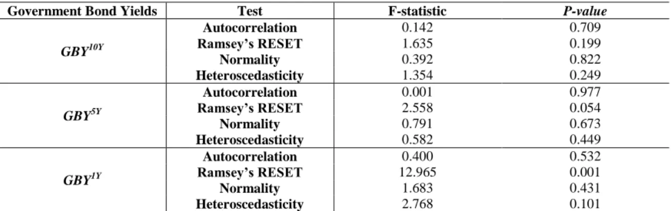
Next, diagnostic tests are carried out (Table 6). We exclude the presence of autocorrelation and confirm that our residuals are normal and homoscedastic. We also confirm that our models are well specified in their functional forms, because the null hypothesis of no misspecification is not rejected. The only exception occurs in the model of the one-year Portuguese government bond yields, for which the null hypothesis of no misspecification is rejected. Nonetheless, this is not considered to be very serious because Ramsey’s RESET test should only be applied when estimates are obtained through the OLS estimator, which is not our case (Agung, 2009). Finally, the plots of the CUSUM and CUSUMSQ tests (Figure A12 and Figure A13 in the Appendix) confirm that the estimated coefficients are stable over time and verify the absence of structural breaks.10 These diagnostic tests show that our models do not suffer from any serious econometric problems; thus, we can proceed with the analysis of the long-term estimates (Table 7) and short-term estimates (Table 8, Table 9 and Table 10) of the Portuguese government bond yields.
Table 6 – Diagnostic tests for our estimates
Government Bond Yields Test F-statistic P-value
GBY10Y Autocorrelation 0.142 0.709 Ramsey’s RESET 1.635 0.199 Normality 0.392 0.822 Heteroscedasticity 1.354 0.249 GBY5Y Autocorrelation 0.001 0.977 Ramsey’s RESET 2.558 0.054 Normality 0.791 0.673 Heteroscedasticity 0.582 0.449 GBY1Y Autocorrelation 0.400 0.532 Ramsey’s RESET 12.965 0.001 Normality 1.683 0.431 Heteroscedasticity 2.768 0.101
Note: Autocorrelation and Heteroscedasticity tests were conducted with 1 lag and Ramsey’s RESET tests were performed with 1 fitted term, albeit results do not change if we had used more lags and more fitted terms, respectively
In the long term and regarding the ten-year Portuguese government bond yields, all the variables are statistically significant at the traditional significance levels, and they have the expected signs. The only exceptions are the variables of fiscal conditions, labour productivity and liquidity risk, which are statistically significant but do not have the expected signs. These counterintuitive results are not unprecedented, because they are also found in other empirical studies on government bond yields. In the case of fiscal conditions, our result is quite controversial, since it indicates that deterioration in the fiscal conditions (i.e. an increase in the
10 Here, we present only the plots of the CUSUM and CUSUMSQ tests for the model of the ten-year
public debt) exerts a negative effect on the Portuguese government bond yields. As argued by Ichiue and Shimizu (2012), this probably happens because the deterioration in fiscal conditions also functions as disinflationary pressure through the expectations of tax hikes (and other austerity measures), which narrow the government bond yields. This mechanism is particularly relevant in Portugal, which belongs to the euro area and is strictly committed to the rules of the Growth and Stability Pact of the European Union Treaty. This implies that any deterioration in the Portuguese fiscal conditions will result in the adoption of austerity measures to comply with the European Union budgetary rules, which ultimately decrease the level of government bond yields through the corresponding recessive and deflationary effects. The conclusion that deterioration in the fiscal conditions would not lead to a higher level of interest rates is also found by Kormendi (1983), Evans (1985, 1986 and 1988), Hoelscher (1986), Makin (1986), McMillin (1986), Aschauer (1989), Darrat (1989 and 1990), Gupta (1989), Findlay (1990), Ostrosky (1990) and Pham (2014). With regard to labour productivity, our result shows that there is a negative relationship between the labour productivity and the Portuguese government bond yields. This could be attributable to the fact that market participants treat an increase in labour productivity as a signal of a higher level of economic growth in the near future, which feeds expectations around the decrease in default risks and consequently favours a decrease in the respective yields. Regarding liquidity risk, a similar result is obtained by Arghyrou and Kontonikas (2012) through a panel data estimation for ten euro area countries (Austria, Belgium, Finland, France, Greece, Ireland, Italy, Portugal, Spain and the Netherlands) as a whole. According to these authors, this positive relationship between liquidity and government bond yields indicates mispricing of liquidity risk. The remaining variables have the expected signs and are in line with other empirical studies on this issue, namely by confirming that macroeconomic performance, foreign borrowing and the inflation rate are positively related to the Portuguese government bond yields and that the demographic situation and global risk aversion are negatively related to them (Ardagna et al., 2007; Haugh et al., 2009; Laubach, 2009; Kumar and Baldacci, 2010; Ichiue and Shimizu, 2012; Dell’Erba and Sola, 2013; Pham, 2014; Poghosyan, 2014; Hsing, 2015).11
With regard to the five-year Portuguese government bond yields, the results do not change dramatically. The only exception is the variable of labour productivity, which loses statistical significance, albeit maintaining a negative sign. The remaining variables are all
11 Note that the long-term and short-term estimates do not change noticeably if we use the primary
balance as a percentage of the gross domestic product or the current account balance as a percentage of the gross domestic product instead of the total general government gross debt as a percentage of gross domestic product as proxies for fiscal conditions. In the same vein, the long-term and short-term estimates do not change substantially if we use the gross external debt as a percentage of the gross domestic product instead of the net external debt as a percentage of the gross domestic product as a proxy for foreign borrowing. All these results are available on request.
statistically significant and exert the same effects as in the model for the ten-year Portuguese government bond yields.
Finally, in relation to the one-year Portuguese government bond yields, the results do not show a radical change. Here, the only exceptions are the variables of macroeconomic performance and liquidity risk, which lose their statistical significance while maintaining their positive signs. Once again, the remaining variables are all statistically significant and exert the same influence as in the model for the ten-year Portuguese government bond yields. This suggests that the vdeterminants of the Portuguese government bond yields are not so particularly different for the different maturities.
Table 7 – Long-term estimates of the Portuguese government bond yields (2000–2016)
Variable GBYt Y 10 Y t GBY5 Y t GBY1 β0 5.575*** 5.668*** 3.796** (1.867) (1.884) (1.568) [2.986] [3.008] [2.420] MPt 0.778** 0.853** 0.650 (0.371) (0.379) (0.398) [2.097] [2.254] [1.633] FCt -0.528*** -0.549*** -0.430*** (0.189) (0.196) (0.149) [-2.792] [-2.806] [-2.877] FBt 0.253** 0.418*** 0.390*** (0.098) (0.128) (0.125) [2.584] [3.267] [3.123] IRt 1.727*** 2.19*** 2.033*** (0.273) (0.309) (0.392) [6.324] [7.095] [5.188] LPt -0.474* -0.526 -1.376** (0.269) (0.319) (0.589) [-1.765] [-1.650] [-2.335] DSt -8.133*** -8.152*** -5.245** (2.736) (2.730) (2.3) [-2.973] [-2.986] [-2.280] GRAt -0.149* -0.282*** -0.430*** (0.077) (0.101) (0.139) [-1.943] [-2.801] [-3.101] LRt 35.709** 27.136** 12.335 (14.505) (12.825) (14.046) [2.462] [2.116] [0.878]
Note: Standard errors in (), t-statistics in [], *** indicates statistical significance at 1% level, ** indicates statistical significance at 5% level and * indicates statistical significance at 10% level
In the short-term, four points should be addressed. Firstly, the coefficients of the error correction terms are strongly statistically significant and have the expected negative signs. This confirms the stability of our three models and their convergence to the long-term equilibrium. The speed of adjustment implies that around 31.6, 36.9 and 44.4 per cent, respectively, of any disequilibrium in the long term are corrected in one quarter. Secondly, the Portuguese
depend positively on their lagged values; this is valid for all three maturities. Borio and McCauley (1996) confirm that this is a well-recognised empirical fact in the literature on asset pricing, highlighting that this sluggishness tends to be greater than in the case of equity prices or even exchange rates. These authors also provide three different explanations to sustain this inertia in the behaviour of government bond yields. The first one corresponds to the pattern of news, according to which there is a reaction to the arrival of news, but this also exhibits persistence by itself. The second one is the digestion of news over time, which is associated with the time of reaction to news by market participants. They reinforce the idea that news can arrive more or less uniformly in time but market participants respond at different speeds; some immediately, and others only with a certain lag. The third one is the memory of market participants. Thirdly, the majority of the remaining variables are also statically significant and have the same signs as in the long term. This seems to confirm that the reaction of the Portuguese government bond yields to these variables are relatively the same in the long term and in the short term. The only exception pertains to the variable of fiscal conditions, which exerts a positive influence on the Portuguese government bond yields in the short term. Fourthly, our models fit especially well the evolution of the Portuguese government bond yields through time, taking into account the high R-squared and adjusted R-squared values, respectively.
Table 8 – Short-term estimates of the ten-year Portuguese government bond yields (2000–2016)
Variable Coefficient Standard Error T-statistic
Y t GBY10 1 0.359*** 0.072 4.983 ∆MPt 0.207*** 0.056 3.675 ∆MPt-1 -0.075 0.059 -1.286 ∆MPt-2 -0.297*** 0.057 -5.243 ∆FCt 0.030 0.042 0.723 ∆FCt-1 0.235*** 0.045 5.225 ∆FCt-2 0.127*** 0.021 5.901 ∆FCt-3 0.097*** 0.023 4.187 ∆FBt -0.044** 0.020 -2.162 ∆FBt-1 -0.073*** 0.022 -3.334 ∆FBt-2 -0.036 0.024 -1.536 ∆FBt-3 -0.073*** 0.022 -3.294 ∆IRt 0.183** 0.081 2.253 ∆IRt-1 -0.061 0.092 -0.663 ∆IRt-2 -0.483*** 0.083 -5.796 ∆LPt -0.125** 0.058 -2.179 ∆LPt-1 -0.070 0.054 -1.286 ∆LPt-2 0.200*** 0.052 3.822 ∆DSt -0.742*** 0.245 -3.032 ∆DSt-1 1.054*** 0.245 4.306 ∆DSt-2 0.397 .0245 1.619 ∆DSt-3 -0.444** 0.198 -2.24 ∆GRAt -0.020** 0.008 -2.527 ∆GRAt-1 0.042*** 0.008 5.256 ∆GRAt-2 0.011 0.007 1.455
∆LRt 2.866 2.215 1.294
∆LRt-1 -7.539*** 2.288 -3.295
ECTt-1 -0.316*** 0.029 -10.678
R-squared = 0.919 Adjusted R-squared = 0.859
Note: ∆ is the operator of the first differences, *** indicates statistical significance at 1% level, ** indicates statistical significance at 5% level and * indicates statistical significance at 10% level
Table 9 – Short-term estimates of the five-year Portuguese government bond yields (2000–2016)
Variable Coefficient Standard Error T-statistic
Y t GBY5 1 0.542*** 0.061 8.862 ∆MPt 0.105 0.077 1.358 ∆MPt-1 -0.108 0.084 -1.284 ∆MPt-2 -0.403*** 0.080 -5.022 ∆FCt -0.042 0.029 -1.439 ∆FCt-1 0.154*** 0.030 5.098 ∆FCt-2 0.258*** 0.031 8.278 ∆FCt-3 0.169*** 0.034 4.989 ∆FBt 0.031 0.030 1.036 ∆FBt-1 -0.042 0.028 -1.478 ∆FBt-2 -0.114*** 0.030 -3.753 ∆FBt-3 -0.097*** 0.031 -3.131 ∆IRt 0.032 0.114 0.280 ∆IRt-1 0.045 0.130 0.349 ∆IRt-2 -0.836*** 0.117 -7.144 ∆LPt -0.154* 0.083 -1.848 ∆LPt-1 -0.105 0.080 -1.310 ∆LPt-2 0.229*** 0.075 3.038 ∆DSt -1.343*** 0.302 -4.441 ∆DSt-1 0.479* 0.278 1.721 ∆DSt-2 0.044 0.284 0.154 ∆DSt-3 -0.645** 0.264 -2.245 ∆GRAt -0.055*** 0.012 -4.690 ∆GRAt-1 0.068*** 0.012 5.768 ∆GRAt-2 0.021* 0.011 1.980 ECTt-1 -0.369*** 0.031 -11.890
R-squared = 0.926 Adjusted R-squared = 0.878
Note: ∆ is the operator of the first differences, *** indicates statistical significance at 1% level, ** indicates statistical significance at 5% level and * indicates statistical significance at 10% level
Table 10 – Short-term estimates of the one-year Portuguese government bond yields (2000–2016)
Variable Coefficient Standard Error T-statistic
Y t GBY1 1 0.577*** 0.095 6.087 Y t GBY1 2 0.472*** 0.115 4.122 Y t GBY1 3 -0.211** 0.097 -2.163 ∆MPt 0.224* 0.132 1.699 ∆MPt-1 -0.265* 0.130 -2.035 ∆MPt-2 -0.384*** 0.127 -3.023 ∆FC -0.068 0.050 -1.365
∆FCt-2 0.260*** 0.057 4.561 ∆FCt-3 -0.180*** 0.058 -3.112 ∆FBt 0.042 0.047 0.891 ∆IRt 0.347* 0.181 1.915 ∆IRt-1 -0.645*** 0.217 -2.971 ∆IRt-2 -0.591*** 0.207 -2.858 ∆LPt -0.537*** 0.149 -3.613 ∆LPt-1 -0.032 0.121 -0.263 ∆LPt-2 0.396*** 0.126 3.153 ∆LPt-3 0.399*** 0.110 3.630 ∆DSt -1.346*** 0.475 -2.837 ∆GRAt -0.095*** 0.021 -4.443 ∆GRAt-1 0.051** 0.020 2.630 ECTt-1 -0.444*** 0.067 -6.666
R-squared = 0.858 Adjusted R-squared = 0.787
Note: ∆ is the operator of the first differences, *** indicates statistical significance at 1% level, ** indicates statistical significance at 5% level and * indicates statistical significance at 10% level
Finally, the economic significance of our long-term statistically significant estimates is presented to improve the identification of each variable’s contribution to the evolution of the Portuguese government bond yields since 2000. As the sovereign debt crisis hit the Portuguese government bond yields quite severely (
Figure
A1
, Figure A2 and Figure A3 in the Appendix), the analysis of the economic significance is performed for four different periods: the pre-crisis period, crisis period, post-crisis period and full period. The dating of each period was carried out taking into account the evolution of the Portuguese government bond yields during that time. Note that the same long-term estimates are used for all four periods given that the hypothesis concerning the existence of structural breaks has already been completely rejected, confirming the stability of our coefficients over time (Figure A12 and Figure A13 in the Appendix). Moreover, the analysis of economic significance is performed only for the ten-year Portuguese government bond yields, not only for simplicity but also because we have already concluded that the determinants of the other two maturities are not particularly different.Table 11 – Economic significance of the long-term estimates of the ten-year Portuguese government
bond yields
Period Variable Long-term
Coefficient
Actual Cumulative
Change Economic Effect
Pre-Crisis Period (2000-2009) MPt 0.778 0.066 0.051 FCt -0.528 0.611 -0.323 FBt 0.253 3.218 0.814 IRt 1.727 0.282 0.487 LPt -0.474 0.436 -0.207 DSt -8.133 0.031 -0.252 GRAt -0.149 -0.003 0.000 LRt 35.709 0.523 18.676 Crisis Period (2010-2013) MPt 0.778 -0.057 -0.044 FCt -0.528 0.497 -0.262 FBt 0.253 0.192 0.049 IRt 1.727 0.077 0.133 LPt -0.474 0.060 -0.028
DSt -8.133 -0.005 0.041 GRAt -0.149 -0.294 0.044 LRt 35.709 0.183 6.535 Post-Crisis Period (2014-2016) MPt 0.778 0.051 0.040 FCt -0.528 -0.020 0.011 FBt 0.253 -0.091 -0.023 IRt 1.727 0.042 0.073 LPt -0.474 0.038 -0.018 DSt -8.133 0.012 -0.098 GRAt -0.149 -0.049 0.007 LRt 35.709 0.021 0.750 Full Period (2000-2016) MPt 0.778 0.062 0.048 FCt -0.528 1.513 -0.799 FBt 0.253 3.807 0.963 IRt 1.727 0.404 0.698 LPt -0.474 0.583 -0.276 DSt -8.133 0.039 -0.317 GRAt -0.149 -0.391 0.058 LRt 35.709 0.901 32.174
Note: The actual cumulative change corresponds to the growth rate of the correspondent variable during the corresponding period.12 The economic effect is the multiplication of the long-term coefficient by the actual cumulative change
For the pre-crisis period, we conclude that the liquidity risk, foreign borrowing, inflation rate and macroeconomic performance were the main drivers of the ten-year Portuguese government bond yields. Effectively, an increase in liquidity, external debt and the inflation rate inflation rate and an acceleration of economic growth favoured a rise in the ten-year government bond yields of 1867.6, 81.4, 48.7 and 5.1 per cent, respectively. Excluding the effect of liquidity, the rise in external debt was the most prejudicial to the evolution of the respective yields and did not compensate for the beneficial effects of the increase in public debt, the active population and labour productivity, which only favoured a decline in these yields of about 32.3, 25.2 and 20.7 per cent, respectively.
During the crisis, liquidity risk, the inflation rate and foreign borrowing remained the main drivers of the ten-year Portuguese government bond yields. In fact, these yields would have been lower by around 653.5, 13.3 and 4.9 per cent if there had not been a rise in liquidity, the inflation rate and external debt, respectively. The beneficial effect of fiscal conditions, which implied a fall in these yields of about 26.2 per cent, was not enough to prevent the rise in these yields during that time.
After the crisis, the effects of each variable on the ten-year Portuguese government bond yields are quite similar to those in the pre-crisis period. The only exception is related to foreign borrowing, which also begins to favour a reduction in these yields, like the active population and labour productivity. Overall, these three variables support a decline in the respective yields of about 2.3, 9.8 and 1.8 per cent. Nonetheless, these effects were clearly supplanted by the
harmful effects linked to the rise in liquidity, the inflation rate and macroeconomic performance, delineated a surge in the respective yields of around 75.0, 7.3 and 4.0 per cent, respectively.
In the full period, we conclude that liquidity risk, foreign borrowing and the inflation rate were the principal drivers of the ten-year Portuguese government bond yields, contributing to an increase of about 3217.4, 96.3 and 69.8 per cent, respectively. These detrimental effects did not compensate for the benefits related to the rise in public debt, the active population and labour productivity, which only favoured a decrease in yields of 79.9, 31.7 and 27.6 per cent, respectively.
Summing up, the Portuguese government bond yields cannot be dissociated from the evolution of the three risk drivers referred to the literature (credit risk, global risk aversion and liquidity risk). All things considered, liquidity risk, the inflation rate and foreign borrowing represent the main triggers of the rise in the Portuguese government bond yields does not compensate for the beneficial effects exerted by the fiscal conditions, the demographic situation and labour productivity.
6. CONCLUSION
This paper constitutes an empirical analysis of the main determinants of the ten-, five- and one-year Portuguese government bond yields by performing a time series econometric analysis of the period between the first quarter of 2000 and the last quarter of 2016.
From a theoretical point of view, the evolution of government bond yields typically depends on three main risk drivers, namely credit risk, global risk aversion and liquidity risk (Manganelli and Wolswijk, 2009; Arghyrou and Kontonikas, 2012; Afonso et al., 2015). Credit risk captures the risk of partial or total default of a sovereign borrower and typically is weighted by incorporating six dimensions (Ichiue and Shimizu, 2012), consisting of as macroeconomic performance, fiscal conditions, foreign borrowing, the inflation rate, labour productivity and the demographic situation (ageing population). Global risk aversion captures the risk appetite and the level of financial risk perceived by market participants. Liquidity risk captures the size and depth of the government bond market and the possibility of capital losses in the event of early liquidation or significant price changes resulting from a small number of transactions in the market.
Accordingly, we estimated three equations for the ten-, five- and one-year Portuguese government bond yields, respectively, using eight independent variables to take into account all