NONLINEAR PREDICTIVE CONTROL OF AN INDUSTRIAL SLURRY
REACTOR
C. H. Fontes
∗M. J. Mendes
†∗Programa de Pós-Graduação em Engenharia Industrial (PEI), Escola Politécnica, Universidade Federal da Bahia,
Salvador, Bahia, Brazil
†Faculdade de Engenharia Química, Universidade Estadual de Campinas, Campinas, São Paulo, Brazil
ABSTRACT
A nonlinear model predictive control (NMPC) is applied to a slurry polymerization stirred tank reactor for the production of high-density polyethylene. Its performance is examined to reach the required mean molecular weight and comonomer composition, together with the temperature setpoint. A com-plete phenomenological model including the microscale, the mesoscale and the macroscale levels was developed to rep-resent the plant. The control algorithm comprises a neural dynamic model that uses a neural network structure with a feedforward topology. The algorithm implementation siders the optimization problem, the manipulated and con-trolled variables adopted and presents results for the regu-latory and servo problems, including the possibility of dead time and multi-rate sampling in the controlled variables. The simulation results show the high performance of the NMPC algorithm based in a model for one-step ahead prediction only, and, at the same time, attests the strong difficulty to control polymer properties with dead time in their measure-ments.
KEYWORDS: Olefin Polymerization, Predictive control, neural networks.
Artigo submetido em 29/03/2007 1a. Revisão em 16/07/2008 2a. Revisão em 04/08/2008
Aceito sob recomendação do Editor Associado Prof. José Roberto Castilho Piqueira
RESUMO
Uma estratégia de controle preditivo não linear é aplicada a um reator tanque agitado de polimerização em lama para a produção de polietileno de alta densidade. O desempenho do controle é analisado no sentido de se obter o peso mole-cular médio numérico, composição de comonômero e tem-peratura desejados. Um modelo fenomenológico completo considerando as micro, meso e macro escalas de modela-gem foi desenvolvido para representar a planta. O algoritmo de controle compreende um modelo interno baseado em re-des neurais com topologia “feedforward”. A implementação do algoritmo contempla o problema de otimização, as va-riáveis manipuladas e controladas adotadas e são apresenta-dos resultaapresenta-dos para os casos de problema servo e regulatório, incluindo-se a possibilidade de tempos mortos e múltiplas taxas de amostragem nas variáveis controladas. Os resulta-dos de simulação mostram o bom desempenho do algoritmo NMPC baseado em um modelo neural treinado para a predi-ção da variável de saída apenas um instante de tempo a frente e, ao mesmo tempo, atestam a dificuldade de controlar dire-tamente as propriedades do polímero com a ocorrência de tempo morto na medição.
1
INTRODUCTION
In the polymerization industry, there is considerable incen-tive to develop real-time optimal strategies that will result in the production of polymers with desired molecular proper-ties. In this sense, the production of polymers with specified end-use properties means that process variables such as tem-perature and molecular weight must be controlled.
The difficult to measure controlled variables, the existence of interactions, dead time and constraints, added to the non-linear and multivariable nature (Schork et al., 1993, Ozkan et al., 2001), pose a challenger problem for the control of polymerization reactor. In many plants, there is a heuristic strategy to control the output process variables. The devel-opment of control strategies for polymerization reactors re-quires an appreciation of what the important properties are and how they relate to variables within the reactor and fur-thermore, what inputs are available. Penlidis et al. (1992) show that simple models that do not require a heavy compu-tational load but capture all the essential process features, are easily amenable to reactor optimization and control studies.
Model Predictive Control (MPC) refers to a class of algo-rithms that compute a sequence of manipulated variable ad-justments in order to optimize the future behavior of a plant. In recent years, there is a considerable literature on the MPC technology, including overviews, industrial applications and its main features (Qin and Badgwell, 1997, 2000, Diehl et al., 2002).
Continuous polymerization processes, such as slurry tech-nology, appear to be suitable for the model predictive con-trol (Rovaglio et al., 2004, Jeong et al., 2001) because, among other things, these processes are multivariable, tightly constrained and typically present a “fat” control problem (Qin and Badgwell, 1997, Schnelle and Rollins, 1998) with more manipulated variables (MV’s) than controlled variables (CV’s), which suggests opportunities for process optimiza-tion also. The nonlinear nature and the large operating regimes with multi-grade productions led to the development of nonlinear model predictive control (NMPC) in which a more accurate nonlinear model is used for process prediction and optimization (Henson, 1998).
Some references present the application of the advanced con-trol algorithms in polymerization systems. Ibrehem et al. (2008) worked with olefin polymerization (ethylene poly-merization) in fluidized-bed catalytic reactors. The authors developed a complete model that takes into account mass and heat transfer between the solid particles and surround-ing gas in the emulsion phase, and also present the applica-tion of neural-network based predictive control for control-ling the temperature of the emulsion system. Other recent work (Gandhi and Mhaskar, 2008) considers the problem of
control a styrene polymerization process subject to input con-straints and destabilizing faults in the control actuators. For the batch and semi-batch polymerization reactors in particu-lar, additional difficulties arise concerning process variables, such as reactor temperature and pressure, which have to fol-low set-point trajectories to assure the quality of the final product. Fontes et al. (2006) show the results and procedures associated with the application of a fuzzy control strategy in a semi-batch reactor for the production of nylon 6, includ-ing variable set-points for pressure and temperature. Nagy et al. (2007) present the benefits of nonlinear model pre-dictive control (NMPC) for the setpoint tracking control of an industrial batch polymerization reactor, considering. Ac-cording to the authors, two different control problems arise in batch process operation, namely, the end-point property con-trol, associated to the product quality at the end of the batch, and the setpoint tracking, associated to the time-varying set-point trajectories. Some references are related to the control of particle size distribution. Dokucu et al. (2008) developed strategies for the regulation of the particle size distribution in a semibatch vinyl acetate (VAc)/butyl acrylate emulsion polymerization system. Three integrated strategies that ex-ploit model reduction to control the PSD (Particle Size Dis-tribution) are presented and compared. The same polymer-ization system was adopted to test a multi-rate model predic-tive controller algorithm to control the full particle size dis-tribution (Dokucu et al., 2008). Embiruçu and Fontes (2006) presented closed-loop results related to the same system de-scribed in Figure 1 considering, in this case, Ziegler-Natta and Phillips catalysis. The authors suggest an approach for the generalized predictive control algorithm, a linear predic-tive controller, to consider multiple sampling rates in the con-trolled variables.
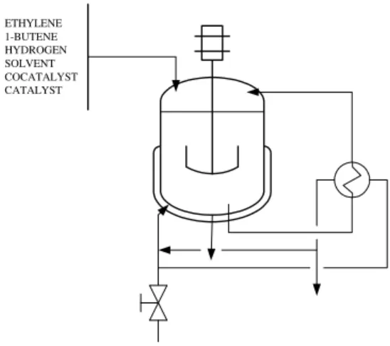
ETHYLENE 1-BUTENE HYDROGEN SOLVENT COCATALYST CATALYST
Figure 1: Schematic representation of the reactor.
The actual state of this process comprises the control of reac-tor temperature and the trial of control the melt index through an heuristic procedure that includes the adjustment of hydro-gen/ethylene ratio in the reactor gas phase. The inexistence of a systematic treatment, the intrinsic complexity of a poly-merization process, marked by its multivariable nature, do not warrant the specification of product with melt index val-ues inside acceptable limits. In this sense, this work treats a control problem that represents an expected increase in the control technology applied to the process described. The control problem comprises the need of expressive reduction in the molecular properties variability through a multivari-able strategy that considers all effects on these properties and establishes directly setpoints for these.
This work presents the problem formulation and simulation results based on a complete phenomenological model of the system (Fontes and Mendes, 2005). An analysis of degree of freedom of this model suggested the establishment of three control variables. In accordance with the process reality and the control problem presented, two polymer properties (aver-age molecular weight and copolymer composition), outputs of phenomenological model, were consider together with the slurry temperature. Additional challenges such as dead time and multi-rate sampling must be analyzed also owing to the direct control of two polymers properties simultane-ously with reactor temperature, whose time constant is much smaller than others.
The optimization problem and simulation results for the reg-ulatory and servo (grade transitions) problems are presented. The neural model was identified to supply only one-step ahead preditions. The simulation tests comprised the anal-ysis of additional aspects such as dead time and multi-rate sampling in the controlled varibales.
Section 2 presents the main aspects related to the
phe-nomenological and neural dynamic models, which are treated in Fontes and Mendes (2001). Finally, section 3 presents the NMPC implementation, pointing out the ma-nipulated and controlled variables, the optimization problem, variables scaling and simulation results.
2
METHODS
The dynamic model
Fontes and Mendes (2001, 2005) present the details about the phenomenological dynamic model used in this work. As dis-cussed in Ray (1991), processes of the heterogeneous catal-ysed olefin polymerization reactors may be decomposed in three levels, namely the microscale (chemical kinetic as-pects), the mesoscale (transport in the particle), and the macroscale (overall mass and energy balance equations) lev-els. This decomposition is used in the present work to con-struct the reactor model. Some simplifying assumptions were adopted such as the slurry volume constant and perfect mix-ing of gas and liquid phases.
At the microscale level, one kinetic mechanism was adopted, according to the coordination polymerization (Kiparissides, 1996), including initiation, propagation, chain transfer and deactivation reactions (see Table 1). Two types of catalytic sites are considered, each one with its own kinetic constants, and the concept of the terminal model for copolymerization (Soares and Hamielec, 1995, 1996) is implicit in the kinetic equations.
ET, BT and CC are ethylene, 1-butene and cocatalyst, re-spectively. The others symbols are commented in Nomen-clature. The procedure employed at the microscale level comprised the generation of balance equations for the living P1j(n, m), P2j(n, m)
and dead polymer chains
(Dj(n, m)), the application of the method of moments (Hutchinson et al., 1992) to enable the mathematical treat-ment of average polymer properties, and the obtaintreat-ment of rate equations for the zero, first and second order moments. Consumption rate expressions for the ethylene, 1-butene, hy-drogen, cocatalyst and active site were obtained also. The kinetic constants (Fontes and Mendes, 2001, 2005) were em-ployed in Arrhenius equation form. Table 2 shows the values of frequency factors for the rate constants. For the activation energies of the propagation, chain transfer and deactivation steps, respectively, the values of 29.4 kJ/mol, 50.2 kJ/mol and 4.2 kJ/mol were taken.
Table 1: Kinetic mechanism for site typej.(j= 1,2)
Initiation:
Pj(0,0) +ET Kpeej
→ P1j(1,0)
Pj(0,0) +BT Kpbb
j
→ P2j(0,1)
Propagation:
P1j(n, m) +ET
Kpeej
→ P1j(n+ 1, m)
P2j(n, m) +ET
Kpbe
j
→ P1j(n+ 1, m)
P1j(n, m) +BT
Kpeb
j
→ P2j(n, m+ 1)
P2j(n, m) +BT
Kpbb
j
→ P2j(n, m+ 1)
Chain Transfer:
P1j(n, m)
Ktsj
→ Pj(0,0) +Dj(n, m)
P2j(n, m)
Ktsj
→ Pj(0,0) +Dj(n, m)
P1j(n, m) +H2
Kthj
→ Pj(0,0) +Dj(n, m)
P2j(n, m) +H2
Kthj
→ Pj(0,0) +Dj(n, m)
P1j(n, m) +ET
Ktmej
→ P1j(1,0) +Dj(n, m)
P2j(n, m) +ET
Ktmbj
→ P1j(1,0) +Dj(n, m)
P1j(n, m) +CC
Ktccj
→ P1j(1,0) +Dj(n, m)
P2j(n, m) +CC
Ktccj
→ P1j(1,0) +Dj(n, m)
Deactivation:
P1j(n, m)
Kdj
→ Cdj+Dj(n, m)
P2j(n, m)
Kdj
→ Cdj+Dj(n, m)
collocation. One material balance on the macropartcile for each specie was developed considering that convective mass transfer inside macropartcile and the instantaneous variation of its volume are negligible.
The assumption of a non-uniform species distribution on the particle established the development of a general local bal-ance (Fontes and Mendes, 2005), providing equations for the moments of chain length distribution and for the active site concentrations.
The macroscale comprised one mass balances for the liquid and gas phases and another for the solid phase, for each one component (ethylene, 1-buthene, hydrogen, solvent and ni-trogen). Overall mass and energy balances were established also.
Table 2: Frequency factors of the kinetic constants
(1/(mol.min))
Site 1 Site 2 Propagation:
Kp,ee 1.101×10⁸ 1.101×10⁸ Kp,be 2.591×10⁶ 1.943×10⁷ Kp,eb 8.290×10⁷ 8.290×10⁷ Kp,bb 1.943×10⁶ 8.031×10⁶ Chain transfer
Kt,s(min−1) 1.615×10⁵ 1.615×10⁵ Kt,h 1.421×10⁸ 1.421×10⁷ Kt,me 3.392×10⁶ 3.392×10⁵ Kt,mb 3.392×10⁶ 1.615×10⁵ Kt,cc 3.876×10⁷ 3.876×10⁶ Deactivation
Kd 3×10⁻¹ 3×10⁻¹
Despite the simulations tests, Table 3 presents the absolute initial values of all inputs variables together with initial val-ues for the weight-average molecular weight (WAMW) and temperature.
Table 3: Initial absolute values for simulation tests. Hydrogen feed flow 10 kg/h
Catalyst feed flow 0.075 kg/h Comonomer feed flow 150 kg/h
Solvent feed flow 16000 kg/h Cocatalyst feed flow 0.2 kg/h
Monomer feed flow 7500 kg/h Water flow in the
reactor jacket 150000 kg/h Water flow in the
external heat exchangers
60000 kg/h
WAMW 122000
Temperature 84.6oC
for use in the predictive control applications.
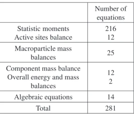
Table 4: Complete dynamic model.
Number of equations Statistic moments
Active sites balance
216 12 Macroparticle mass
balances 25
Component mass balance Overall energy and mass
balances
12 2
Algebraic equations 14
Total 281
The procedure adopted to obtain the neural models, used in the predictive control algorithm, is presented in Fontes and Mendes (2001). The neural network structure consists of a feedforward topology with only one hidden layer and gives one-step ahead prediction. The tangent hyperbolic function was used in the hidden neurons and the linear function was used in the output layer. The training was accomplished us-ing the Levenberg-Marquadt algorithm with a learnus-ing rate equal to 0.01 and the initial value for the Hessian adjustment parameter was assumed equal to 0.9. A batch training proce-dure was applied considering the minimization of the mean squared error of each epoch.
The identification was conducted adopting one neural model for each process output that can be represented by a NARX (Nonlinear AutoRegressive with eXogeneous inputs) struc-ture (Su and McAvoy, 1997, Doherty et al., 1997). The MISO (Multiple Input Single Output) model, for each output, con-siders all process inputs (feed rates of ethylene, catalyst, co-catalyst, 1-butene, hydrogen, solvent and refrigeration wa-ter), and one value of dead time for each input variable had to be adopted also. Two data samples (training and test), pro-vided from the phenomenological model (sampling period of 5 min), were adopted for the identification and a cross vali-dation procedure was adopted in order to select the best num-ber of hidden neurons for each MISO model, considering a maximum number of 2000 training epochs. As it was to be expected, in the nonlinear case a neural model with a feed-forward structure leads to results that are more accurate for short prediction horizons than for long prediction horizons. Multi-step ahead prediction is however necessary to imple-ment predictive control schemes.
2.1
Nonlinear model based control
algo-rithm
The predictive control algorithm for the slurry reactor has the following features:
• Multiple inputs and multiple controlled variables.
• Simultaneous resolution of the optimization problem.
• Internal model comprising one neural model for each control variable (MISO model) that includes all the ma-nipulated variables adopted.
An analysis of the phenomenological model conducted to achievement of 3 degrees of freedom for this and 3 variables were selected to be controlled:
• Reactor temperature (Tr).
• Weight-average molecular weight (Mw).
• Average fraction of comonomer incorporated into the polymer (XBT).
This set of controlled variables poses additional challenges for the control problem. First, there is the possibility of con-siderable dead time in the measurement of outputs associated with the polymer properties (Mw and XBT) owing to the slurry transport, drying and the analysis time. Second, pro-cess variables such as temperature have a dynamic response typically speed regard to the polymer properties, which sug-gests the existence of multi-rate sampling in the controlled variables. The closed loop simulation comprised the addi-tional analysis of these two effects (dead time and multi-rate sampling) on the control algorithm performance.
8 (eight) manipulated variables were adopted comprising feed rates to the reactor and water flows related to the re-frigeration system:
• Ethylene massic flow (FET).
• Buthene massic flow (FBT).
• Catalyst massic flow (FC).
• Cocatalyst massic flow (FCC).
• Hydrogen massic flow(FH2).
• N-hexane massic flow (FN X).
• Water flow to the reactor jacket (FW C).
2.2
Optimization problem
Besides the nonlinear nature of plant, a nonlinear internal model suggests also the possibility of a more efficient con-troller, able to accomplish grade transitions, without changes the catalytic system. These grade transitions are common in the system studied and imply in an expressive change of the operation point.
Adopting the controlled and manipulated variables listed in the previous section, the predictive control algorithm com-prises the following nonlinear programming problem, which must be solved at each sampling period to generate the con-trol moves.
Objective function
min
u(t) E(t) =
P X k=1
ke(t+k)k2R !
+
M X k=1
k∆u(t+k−1)k2Q !
, (1)
where the norm terms meankxk2Z =x
T ·Z·x
, andtis the current instant.
The control moves of each one MV
(u≡FET, FBT, FC, FCC, FN X, FH2, FW C, FW T) are achieved as follows:
∆u(l) =u(l)−u(l−1), ifl > t, (2)
∆u(l) =u(l)−u(t−1), sel=t, (3)
and the deviations from a desired response, over a predic-tion horizon of length P must be achieved for each controlled variable(y≡Tr, Mw, XBT):
e(t+k) =yref(t+k)−[ˆy(t+k) +d], (4)
whered=y(t)−yˆ(t).
Despite the options for specifying future CV behavior (Qin and Badgwell, 1997), reference trajectory was adopted in this work and a first order curve is drawn from the current CV value to the setpoint according to the following expression:
yref(t+k) =αk·y(t) +ysp(t)· 1−αk
,k= 1, . . . , P (5)
αis the time constant that establishes the response speed.
Constraints
Regarding to the input variables, the following constraints must be considered:
ui≤u(t+k−1)≤us,k= 1, . . . , M, (6)
∆ui≤∆u(t+k−1)≤∆us,k= 1, . . . , M. (7)
Hard constraints are also considered for the output predic-tions:
yi ≤yˆ(t+k)≤ys,k= 1, . . . , P, (8)
where (u≡FET, FBT, FC, FCC, FN X, FH2, FW C, FW T) and(y≡Tr, Mw, XBT).
The model constraints comprises the MISO neural model identified for each CV, whose structure presents all the MV’s. Each CV contributes with P equality constraints expressed as follows:
ˆ
y(t+1) =Fy
y(t), y(t−1), . . . ,
y(t−ny+ 1), FET(t), . . . , FET(t−1−nETy + 2), . . . ,
FW T(t), . . . , FW T(t−1−nW Ty + 2)
(9) ˆ
y(t+ 2) =Fy ˆ
y(t+ 1), y(t), . . . , y(t−nMw+ 2),
FET(t+ 1), . . . ,
FET(t−1−nET y+ 3), . . . , FW T(t+ 1), . . . , FW T(t−1−nW T y+ 3)
(10) .. . ... ... ˆ
y(t+P) =Fy ˆ
y(t+P−1),yˆ(t+P−2), . . . , y(t), . . . , y(t−nMw+P),
FET(t+P−1), . . . , FET(t−nET y+P), . . . , FW T(t+P−1), . . . , FW T(t−nW T y+P)
The optimization problem presented has 8×M+3×P decision variables (output predictions were also considered decision variables in the problem formulation) and 8×M degrees of freedom that is equal to the number of present and future values of MV’s.
2.3
Scaling variables
In the system studied, there are enormously differences in the typical values of MV’s and CV’s that should be consid-ered in the penalty adjustments (weight matricesQandR)
for the control tuning (Meadows and Rawlings, 1997). In this sense, the scaling by variable transformation (Gill et al., 1981) should be useful and provides certain desirable prop-erties during the optimization process.
All the decision variables presented in the optimization prob-lem were scaled trough the use of dimensionless deviation variable (ddv):
vad= v−vss
vss , (12)
wherevssis the initial steady state considered in the simula-tion tests.
2.4
Tuning procedure
The strategy employed for the tuning parameters adjustments comprised the following aspects:
• Only the move suppression factors and horizons were adjusted.
• The penalties on the deviations from the desired re-sponse (matrixR)were fixed at 20 for all CV’s.
• The time constant of the reference trajectory was fixed at 0.5 for all CV’s.
• The weights of each control move and output prediction deviations were assumed constant along the prediction horizon.
The limits used for all MV’s are in agreement with the data range adopted during the neural models training (section 3). Based on the melt index and density specifications and on the operational practice, bounds were established for each CV (table 5), regarding to its current setpoint.
The grade transitions simulations (servo problems) establish changes in the output bounds or specifications. In this sense, it was proposed the use of two trajectories to represent the
Table 5: Output specifications.
Variable Bounds
Tr ± 1 %
Mw ± 3 %
XBT ± 5 %
bounds of each output during the grade transition. Consider-ing the use of hard constraints for the CV’s predictions (Eq. 8), the trajectory parameters in each case were always ad-justed to reduce the effect of the output bounds on the op-timization problem. Hence, in the case of setpoint increase, the upper and lower trajectories must be speedy and sluggish, respectively. In the case of setpoint decrease the opposed is applied.
2.5
Measurement delay in the outputs
The occurrence of a dead time equals to θu sampling in-tervals in some CV measurement leads to increase the pre-diction horizon owing to the inclusion of present and fu-ture MV’s values only after the firstθu output predictions. To prove this fact, consider a SISO case where the internal model is represented as follows:
ˆ
y(t+ 1) =F(u(t), y(t)).
Considering thatym is the measured value from the plant and that this measurement has a delay equals toθu, the pre-dictions obtained at timetare:
ˆ
y(t+ 1) =F(u(t−θu), ym(t)), (13)
ˆ
y(t+ 2) =F(u(t−θu+ 1),yˆ(t+ 1)) (14) ..
.
ˆ
y(t+θu) =F(u(t−θu+θu−1),yˆ(t+θu−1))(15),
ˆ
y(t+θu+ 1) =F(u(t),yˆ(t+θu)), (16)
ˆ
y(t+θu+ 2) =F(u(t+ 1),yˆ(t+θu+ 1)), (17) ..
.
ˆ
y(t+θu+P) =F(u(t+θu+P −1),
ˆ
y(t+θu+P−1)) (18)
In some tests with a long prediction horizon, only a subset of predictions, called coincident points (Qin and Badgwell, 1997), is selected and used in the optimization problem.
2.6
Simulations tests and discussion
The simulation tests were conducted in two steps compris-ing the servo and regulatory problems. First, the controller performance was analyzed considering one grade transition without change in the catalytic system. For the regulatory problem tests, the ability to reject some potential distur-bances and to keep controlled variables in their setpoints were verified.
In all tests, the process is represented by the phenomenolog-ical model (Fontes and Mendes, 2001) and the control action interval is always equals to 5 min.
2.6.1 Servo problem
In this section, simultaneous setpoint changes in the con-trolled variables were applied according to table 6. Changes in the specification limits were also imposed and the strategy described in section 3.3 had to be used.
Table 6: Setpoint changes (grade transition).
Variable initial setpoint (ddv))
end setpoint (ddv)
Tr 0 0.069
Mw 0 -0.123
XBT 0 0.069
The tests comprised two cases:
• Setpoint changes considering multi-rate sampling in the controlled variables. Measurement intervals of 5 min and 40 min were adopted for the temperature and poly-mer properties (MwandXBT), respectively.
• Setpoint changes with a dead time equals to 30 min ow-ing to delay in the molecular weight and comonomer content measurements.
Despite the tuning procedure, an initial standard tuning was employed as a reference for the adjustments in each case. This standard tuning (table 7) provides an excellent control performance in the absence of multi-rate sampling and mea-surement delay in the outputs.
a) Servo problem with multi-rate sampling
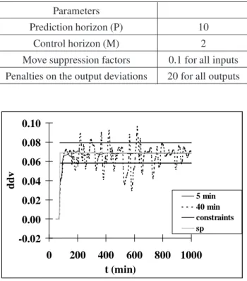
Table 7: Standard tuning.
Parameters
Prediction horizon (P) 10
Control horizon (M) 2
Move suppression factors 0.1 for all inputs Penalties on the output deviations 20 for all outputs
-0.02 0.00 0.02 0.04 0.06 0.08 0.10
0 200 400 600 800 1000
t (min)
d
d
v
5 min 40 min constraints sp
Figure 2: Temperature. Measurement intervals of 5 and 40 min for bothMwandXBT. P=10, M=2 and control move weights equal to 0.1.
Figures 2-3 present simulation results with measurement intervals of 5 and 40 min for both molecular weight and comonomer content. In both cases, the standard tuning (table 7) was employed. Results show a sensible drop in the con-trol performance with the occurrence of ringing (excessive oscillations) between sample points, owing to the increase in the measurement interval for the polymer properties (Mw andXBT). On the other hand, Figure 4 shows that the per-formance improvement can be easily achieved through the increase in the prediction horizon and weights of control moves.
Some results presented show the occurrence of CV’s values outside the specification limits (constraints). This fact is not related with the achievement of unfeasible solution for the optimization problem, since the hard constraints established according to Eq. (8) are imposed in the output predictions.
b) Servo problem with dead time
-0.20 -0.15 -0.10 -0.05 0.00
0 200 400 600 800 1000
t (min)
d
d
v
5 min 40 min constraints sp
Figure 3: Molecular weight. Measurement intervals of 5 and 40 min for bothMwandXBT. P=10, M=2 and control move weights equal to 0.1.
Figure 4: Molecular weight. Measurement intervals of 40 min for bothMwandXBT. M=2 and control move weights equal to 0.5.
strong effect of dead time (“dt”) on the control performance, with the occurrence of unstable behavior.
Despite the bad results achieved with the standard tuning, a sensible improvement can be obtained with a prediction horizon equals to 70 and weights of 0.5 or 1 for the control moves (Figure 6).
2.6.2 Regulatory problem
Temperatures of ethylene and solvent feed streams were con-sidered as potential disturbances. No one setpoint change in the controlled variables was applied in this case.
Figures 7 and 8 present the temperature and comonomer
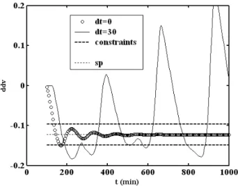
con-Figure 5: Molecular weight. Servo problem results without and with dead time of 30 min in theMwandXBT. P=10, M=2 and control move weights equal to 0.1.
-0.20 -0.15 -0.10 -0.05 0.00
0 500 1000 1500 2000
t (min)
d
d
v
0.5 1 constraints sp
Figure 6: Molecular weight. Servo problem results with dead time of 30 min in theMwandXBT. P=70, M=2 and control move weights equal to 0.5 and 1.
tent profiles considering a dead time of 30 min in the polymer properties measurements, and the using of standard tuning (table 7). This test comprised the input of step perturbations of 20 % and 30 % on the ethylene and solvent temperatures, respectively. One more time, it can be detected a bad control performance with closed loop instability.
-0.02 -0.01 0.00 0.01 0.02
0 200 400 600 800
t (min)
d
d
v
constraints sp
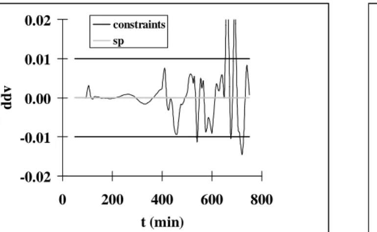
Figure 7: Temperature. Regulatory problem results with dead time of 30 min in theMw andXBT. P=10, M=2 and control move weights equal to 0.1.
-0.06 -0.04 -0.02 0.00 0.02 0.04 0.06
0 200 400 600 800
t (min)
d
d
v
constraints sp
Figure 8: Comonomer content. Regulatory problem results with dead time of 30 min in theMwandXBT. P=10, M=2 and control move weights equal to 0.1.
2.6.3 Uncertainty of dead time
Since the measurement delay in a real process is not exactly known and can vary over a very wide range, an uncertainty of this must be accounted in designing an NMPC controller.
Applying weights of 0.5 for the each control moves and the same horizons, Figures 10-11 present results with differences between the internal model dead time and the dead time ef-fectively practiced in the process. A regulatory problem was considered with the input of a pulse perturbation on the sol-vent feed temperature. The results show that it is possible to achieve good performance even with a model dead time equals to 1 hour and a measurement delay in the process equals to 30 min. This also attests the robustness of the pre-dictive control algorithm and denotes that the control
perfor--0.02 -0.01 0.00 0.01 0.02
0 200 400 600 800
t (min)
d
d
v
0.5 1 constraints sp
Figure 9: Temperature. Regulatory problem results with dead time of 30 min in the MwandXBT. P=70, M=2 and control move weights equal to 0.5 and 1.
-0.06 -0.04 -0.02 0.00 0.02 0.04 0.06
0 500 1000 1500
t (min)
d
d
v
plant=0.5h model=1h plant=1h model=0.5h constraints
sp
Figure 10: Molecular weight. Regulatory problem results with dead time error in the internal model. P=70, M=2 and control move weights equal to 0.5.
mance, just as in the preceding sections, is directly related to increase of dead time practiced in the polymer properties measurements.
3
CONCLUSIONS
-0.06 -0.04 -0.02 0.00 0.02 0.04 0.06
0 500 1000 1500
t (min)
d
d
v
plant=0.5h model=1h plant=1h model=0.5h constraints
sp
Figure 11: Comonomer content. Regulatory problem results with dead time error in the internal model. P=70, M=2 and control move weights equal to 0.5.
weights established for the output deviations.
The proposed control scheme represents advancement with regard to the actual scheme, enabling the effective control of macromolecular properties at desired values. Despite the other procedures previously published, based in a linear in-ternal model, the use of NMPC enables the implementation of a more efficient controller, able to drive servo problems featured by large grade transitions. In this sense, this work also presents a proved strategy to handle the output restric-tions during the transition.
The presence of considerable dead time or multi-rate sam-pling in the output measurements increases the complexity of the control problem. In this sense, the tuning procedure pro-posed in this work, comprising only the control move penal-ties and horizons adjustments, was capable to control all the outputs and enough to warrant the closed loop stability.
Still without dead time and multi-rate sampling, the excellent performance of NMPC together with the process stabiliza-tion through the use of long predicstabiliza-tion horizons show that the internal neural model, trained for one step ahead prediction only, is perfectly suitable for the predictive control applica-tions.
The presence of considerable delay in the polymer proper-ties measurements produces a more complex control prob-lem than with the existence of only multi-rate sampling. Al-though the adjustments of control move weights and/or pre-diction horizon were efficient in this case, the uncertainty and variability of dead time establishes the need of on-line esti-mators for the molecular weight and comonomer content that provide values of these outputs in the slurry stream. The suc-cess of a NMPC algorithm, applied to a slurry reactor and
with direct control of mean molecular properties, depends strongly in how these variables must be measured or esti-mated.
Without the inclusion of dead time effect, the simulation re-sults show that a control horizon equals to 2, a prediction horizon between 10 and 20 and control move weights equal to 0.5 can achieve satisfactory performance of NMPC for the system analyzed.
Another stage of polymerization engineering of this system could be reached through a direct control of end-use prop-erties such as stiffness, impact strength and glass transition temperature, or definition of optimal operation conditions to achieve the desired values for these (reverse polymerization). In both cases, more complex relations, multivariable, must be determined between end-use and molecular properties such as molecular weight distribution (Latado et al., 2001, Valap-pil J. and Georgakis C., 2002, Farkas et al., 2004, Grosso and Chiovetta, 2005 and Asteasuain et al., 2003).
ACKNOWLEDGMENTS
The authors acknowledge the financial support provided by CNPq through a grant to C. Fontes as well as the technical support from Braskem Petrochemical Company.
NOMENCLATURE
Cd deactivated site.
D(n, m) dead polymer chains withnmonomer units andm comonomer units, mol/l;
d disturbance term used in conventional MPC feedback;
e deviations from the reference trajectory;
Fi feed flow rate of componenti, ton/h;
k time in discrete system;
Kpee, Kpbb propagation rate constants,l/(mol·min);
Kpeb, Kpbe propagation rate constants,l/(mol·min);
Kts rate constant forβ-hydride elimination, min−1;
Kth rate constant for transfer to hydrogen,l/(mol·min);
Ktme rate constants for transfer to monomer, l/(mol·min);
Ktmb rate constants for transfer to monomer, l/(mol·min);
Ktcc rate constant for transfer to cocatalyst,l/(mol·min);
Mw weight-average molecular weight;
M control horizon;
ny number of output values in the neural network input layer;
nuy number of past values of inputuin the MISO model for outputy;
P prediction horizon;
P1(n, m) living polymer chains withnmonomer units and
mcomonomer units, with terminal monomer;
P2(n, m) living polymer chains withnmonomer units and
mcomonomer units, with terminal comonomer;
P(0,0) active site;
td dead time;
Tr reactor temperature,oC;
t time;
u manipulated variable;
XBT average fraction of comonomer incorporated into the polymer;
y real process output (controlled variable);
ˆ
y model output;
yref reference trajectory in MPC objective;
ysp setpoint of outputy;
∆u control move;
θu dead time of output related to inputu;
α trajectory time constant;
Subscripts:
ET ethylene;
BT 1-butene;
C catalyst;
CC cocatalyst;
N X solvent (n-hexane);
H2 hydrogen;
W C water to the reactor jacket;
W T water to the external heat exchangers;
i lower bound;
s upper bound.
j site type
ss steady state;
Superscripts:
j site type;
ad dimensionless variable.
Abbreviations
sp setpoint.
dt dead time.
MISO Multiple Input Single Output.
ddv dimensionless deviation variable.
CV controlled variable.
MV manipulated variable.
REFERENCES
Asteasuain, M., Pérez, M. V., Sarmoria, C. and Brandolin, A., “Modeling Molecular Weight Distribution, Vinyl Content and Branching in the Reactive Extrusion of High Density Polyethylene”, Latin American Applied
Research, 33, 241-249, (2003).
Diehl, M, Bock, H. G., Shloder. J. P., Findeisen, R., Nagy, Z., Allgower, F., ”Real-time Optimization and Nonlin-ear Model Predictive Control of Processes Governed by Differential-Algebraic Equations”, J. Process Control, 12, 577-585 (2002).
Doherty S. K., Gomm J. B. and Williams D., “Experiment Design Considerations for Non-Linear System Identifi-cation Using Neural Networks”,Computers Chem. En-gng, vol. 21, no3, 327-346, (1997).
Dokucu, M. T., Park, Myung-June and Doyle F. J., “Multi-Rate model predictive control of particle size distribu-tion on a semibatch emulsion copolymerizadistribu-tion reac-tor”,Journal of Process Control, 18, 105-120, (2008).
Embiruçu, M. and Fontes, C., “Multirate multivariable gen-eralized predictive control and its application to a slurry reactor for ethylene polymerization”,Chemical
Engi-neering Science, 61, 5754-5767, (2006).
Farkas, E., Meszena Z. G. and Johnson, A., “Molecular Weight Distribution Design with Living Polymeriza-tion ReacPolymeriza-tions”, Industrial & Engineering Chemistry
Research, 43, 7356-7360, (2004).
Floyd S., K. Y.Choi , T. W. Taylor and W. H. Ray, “Poly-merization of Olefins Through Heterogeneous Cataly-sis. III. Polymer Particle Modelling with an Analysis of Intraparticle Heat and Mass Transfer Effects”,J. Appl.
Polym. Sci., 32, 2935-2960, (1986).
Fontes, C. and Embiruçu, M., “Multivariable Correlation Analysis and Its Application to an Industrial Polymer-ization Reactor”,Computers & Chemical Engineering, 25, 191-201, 2001.
Fontes C. and Mendes M., “Modeling and Simulation of an Industrial Slurry Reactor for Ethylene Polymerization”,
Latin American Applied Research, 31, 345-352, (2001).
Fontes, C. H. and Mendes, M. J., “Analysis of an Indus-trial Continuous Slurry Reactor for Ethylene-Butene Copolymerization”,Polymer, 46, 2922-2932, (2005).
Fontes, C. H. O., Wakabayashi, C. and Embiruçu, M., “Anal-ysis and Fuzzy Control of a Polymerization Reactor for Production of Nylon 6”, In: XXII Interamerican Congress of Chemical Engineering, Buenos Aires, v. 1, 30-31, (2006).
Ghandi, R. and Mhaskar, P., “Safe-parking of nonlinear pro-cess systems”, Computers and Chemical Engineering, 32, 2113-2122, (2008).
Gill P. E., Murray W. and Wright M. H., “Practical Optimiza-tion”, Academic Press, Inc., (1981).
Grosso, W. E. and Chiovetta, M. G., “Modeling a Fluidized-Bed Reactor for the Catalytic Polymerization of Ethy-lene: Particle Size Distribution Effects”.Latin
Ameri-can Applied Research, 35, 67-76, (2005).
Henson M. A., “Nonlinear Model Predictive Control: Cur-rent Status and Future Directions”,Comput. Chem. En-gng., vol. 23, 187-202, (1998).
Hutchinson R. A., C. M. Chen and W. H. Ray, “Polymer-ization of Olefins Through Heterogeneous Catalysis. X. Modeling of Particle Growth and Morphology”, J.
Appl. Polym. Sci., 44, 1389-1414, (1992).
Ibrehem, A. S., Hussain, M. A. and Ghasem, N. M., “Math-ematical Model and Advanced Control for Gas-Phase Olefin Polymerization in Fluidized-bed Catalytic Re-actors”,Chinese Journal of Chemical Engineering, 16 (1), 84-89, (2008).
Jeong, B. G., Yoo K. Y. and Rhee H. K., “Nonlinear Model of a Continuous Methyl Methacrylate Polymer-ization reactor”, Industrial & Engineering Chemistry
Research,40, 5968-5977, (2001).
Kiparissides C., “Polymerization Reactor Modeling: A Re-view of Recent Developments and Future Directions”,
Chem. Eng. Sci., 51( 10), 1637-1659, (1996).
Latado, A., Embiruçu, M., Mattos, A. G., Pinto, J. C., “‘Modeling of end-use Properties of Poly(propylene/ethyelene) Resins”, Polymer Test-ing, 20, 419-439, (2001).
Meadows E. S. and Rawlings J. B., in Henson M. e Seborg D., “Nonlinear Process Control”, Prentice-Hall, Inc., (1997).
Nagy, Z. K., Mahn, B., Franke, R. and Allgower, F., “Eval-uation study of an efficient output feedback nonlinear model predictive control for temperature tracking in an industrial batch reactor”, 15, 839-850, (2007).
Ozkan G., Ozen S., Erdogan S., Hapoglu H and Alpbaz M, “Nonlinear Control of Polymerization Reactor”,
Com-put. Chem. Engng.,vol. 25, 757-763, (2001).
Penlidis, A., Ponnuswamy, S. R., Kiparissides, C., and O’Driscoll, K. F., “Polymer Reaction Engineering: Modelling Considerations for Control Studies”, The
Chemical Engineering Journal, 50, 95-107, (1992).
Qin S. J. and Badwell T. A., “An Overview of Industrial Model Predictive Control Technology”, Aiche Symp. Ser., 93, 232-256, (1997).
Qin S.J. and Badgwell, T.A., “An Overview of Nonlinear Industrial Model Predictive Control Applications”. In: Nonlinear Model Predictive Control. Allgöwer, F., A. Zheng (Eds.).Progress in Systems and Control Theory
Series, v. 26, Switzerland: Birkhauser Boston, (2000).
Ray W. H., "Modelling of Addition Polymerization Pro-cesses",Can. J. Chem. Eng., 69, 626-629 (1991).
Rovaglio, M., Algeri, C and Manca D., “Dynamyc Model-ing of a Poly (ethyelene terephtalate) Solid-State Poly-merization Reactor II: Model Predictive Control”,
In-dustrial & Engineering Chemistry Research, 40,
Schnelle P D. and Rollins D., “Industrial Model Predictive Control Technology as Applied to Continuous Poly-merization Processes”,ISA Transactions, vol. 36, no 4, 281-292, (1998).
Soares J. B. P. and A. E. Hamielec, “General Dynamic Mathematical Modelling of Heterogeneous Zielger-Natta and Metallocene Catalyzed Copolymerization with Multiple Site Types and Mass and Heat Trans-fer Resistances”,Polymer Reaction Engineering, 3(3), 261-324, (1995).
Soares J. B. P. and A. E. Hamielec, “”Copolymerization of Olefins in a Series of Continuous Stirred-tank Slurry-Reactors using Heterogeneous Ziegler-Natta and Met-allocene Catalysts. I. General Dynamic Mathematical Model”,Polymer Reaction Engineering, 4(2&3), 153-191, (1996).
Su H. T. and McAvoy T. J., in Henson M. e Seborg D., “Non-linear Process Control”, Prentice-Hall, Inc., (1997).
Valappil, J., Georgakis, C., “Nonlinear Model Predictive Control of end-use Properties in Batch Reactors”,