J. Braz. Comp. Soc. vol.7 número1

Using Q uantitative Information for E

Using Q uantitative Information for E

Using Q uantitative Information for E

Using Q uantitative Information for Ef-

f-

f-

f-ficie nt

ficie nt

ficie nt

ficie nt

A

A

A

As

s

s

ssociation R ule G e ne ration

sociation R ule G e ne ration

sociation R ule G e ne ration

sociation R ule G e ne ration

Bruno Pôssas, Wagner Meira Jr., Márcio Carvalho and Rodolfo Resende

Bruno Pôssas, Wagner Meira Jr., Márcio Carvalho and Rodolfo Resende

Bruno Pôssas, Wagner Meira Jr., Márcio Carvalho and Rodolfo Resende

Bruno Pôssas, Wagner Meira Jr., Márcio Carvalho and Rodolfo Resende

Department of Computer Science

Federal University of Minas Gerais

Belo Horizonte – MG – Brazil

{bavep,meira,mlbc,rodolfo}@dcc.ufmg.br

Abstract

Keywords: Data mining, association rules, algorithms, knowledge discovery in databases.

1 Introduction

The problem of mining association rules in categori-cal data presented in customer transactions was intro-duced by Agrawal, Imielinski and Swami [2]. This semi-nal work gave birth to several investigation efforts [4,13] resulting in descriptions of how to extend the original concepts and how to increase the performance of the related algorithms.

The original problem of mining association rules was formulated as how to find rules of the form set1 !set2. This rule is supposed to denote affinity or

correla-tion among the two sets containing nominal or ordinal data items. More specifically, such an association rule

should translate the following meaning: customers that buy the products in set1 also buy the products in set2. Statistical basis is represented in the form of minimum support and confidence measures of these rules with respect to the set of customer transactions.

The original problem as proposed by Agrawal et al.[2] was extended in several directions such as adding or replacing the confidence and support by other measures, or filtering the rules during or after generation, or includ-ing quantitative attributes.

Srikant and Agrawal [16] describe a new approach where quantitative data can be treated as categorical. This is very important since otherwise part of the customer transaction information is discarded.

checked in terms of its performance. The algorithm effi-ciency is linked to the size of the database that is amena-ble to be treated. Therefore it is crucial to have efficient algorithms that enable us to examine and extract valuable decision-making information in the ever larger databases.

In this paper we present an algorithm that can be used in the context of several of the extensions provided in the literature but at the same time preserves its performance, as demonstrated in a case study. The approach in our algorithm is to explore multidimensional properties of the data (provided such properties are present), allowing us to combine this additional information in a very efficient pruning phase. This results in a very flexible and efficient algorithm that was used with success in several experi-ments using categorical and quantitative databases.

The paper is organized as follows. In the next section we describe the quantitative association rules and we present na algorithm to generate it. Section 3 presents an optimization of the pruning phase of the Apriori [4] algo-rithm based on quantitative information associated with the items. Section 4 presents our experimental results for mining four synthetic workloads, followed by some re-lated work in Section 5. Finally we present some conclu-sions and future work in Section 6.

2 Quantitative Rules

Items found in relational tables have many different attributes. These attributes may be either quantitative (such as age or salary) or categoric (such as zip code, a boolean value or a license plate number). In this work, any valued attribute will be treated as quantitative and will be used to derive the quantitative association rules presented in this section.

2.1 Formal Definition

Let A = {a1, a2, ..., an} be the set of attributes from a table

and V the set of non-negative values for an attribute, and Va

be the set of values for an attribute a. We define an item i as the pair 〈a,qa〉, where a is an attribute and qa∈ Va its

quantita-tive value. An itemrange is the contiguous allowable range for an attribute a, represented by a tuple 〈a: la - ha〉 where la∈

Va, ha ∈ Va, and la≤ ha are its low and high limits. We

ob-serve that, for each attribute, only a single range is allowed. It may be interesting to consider the case of multiple non-overlapping ranges but this is for further work.

Let us represent a transaction T as the set {t1, t2,...tn}

of its items and by D the set of all transactions. A transac-tion Tsatisfies a given set of em itemranges I, if for each 〈aI : la - ha〉∈I there exists an 〈aT, qa〉∈T with aI = aT e la≤

qa≤ ha. A quantitative association rule is an expression of

the form X ! Y, where X ⊂ I, Y⊂ I, X ∩ Y = ∅ and I is

a set of itemranges. As defined in [2], a rule

X ! Y is valid for the transaction set D with confidence c if c% of the transactions in D that satisfy X also satisfy Y. The rule X ! Y has support s in the transaction set D if s of the transactions in D satisfy X ∪ Y. Given a transac-tion set D, the quantitative association rule generation problem is the problem of generating all rules that have support and confidence greater than some given con-stants, denoted by minsupp and minconf, respectively.

As an example of application of this rule, consider the supermarket purchase analysis problem. In this model, a transaction is a set of items bought by a customer. A rule may be: “80% of the people who bought between 1 and 5 beers also bought between 2 and 4 bags of potato chips”. This information may be strategic when investing in a new advertisement campaign or designing a new layout for the store.

For the sake of this presentation, the solution of the quantitative association rule generation problem is divided into three steps: The first step consists of enumerating the support for the itemranges sets. The second step consists of finding all the itemrange sets that have support values greater than minsupp (these are the frequent or large sets). The last step consists of generating the association rules derived from the frequent sets found in the second step. These steps are the same those of the non-quantitative procedure, but the extra information about the quantities induces an additional dimension on the generated rules, which usually increases the rules' information content.

2.2 Generating Quantitative Rules

In this subsection we describe the algorithm for gen-erating quantitative association rules. The starting point of our algorithm is counting the itemranges in the data-base, in order to determine the frequent ones. These fre-quent itemranges are the basis for generating higher-order itemranges using an algorithm similar to Apriori.

We consider the size of a transaction as the number of items that it comprises. We define as a k-itemset a set of items of size k and denote frequent (large) itemsets by Lk

and candidate itemsets (possibly frequent) Ck. A

j-rangeset is a set of j-itemranges, and each k-itemset has a j-rangeset that stores the quantitative rules of the itemset.

Once we determine all frequent sets and their quanti-tative ranges, the association rules are generated. The general outline of the algorithm is presented in Figure 1. The syntax and semantics of the primitives employed in our algorithm are similar to other approaches in the litera-ture. A short description of the data structures is pre-sented in the next subsection.

1. L₁ = {frequent 1 – itemsets};

2. For (k = 2; Lk-1≠ 0; k + +) {

3. C_k = generate_candidates (L _k-1);

4. ∀ transactions T ∈ DB

5. ∀ subsets t ∈ T

6. If (c ∈ Ck: c is valid in t) then c.count ++;

7. Lk = { c ∈ Ck | c.count ≥ minsup};

8. }

9. ∀ Lk, k > 2

10. generate_rules (L_k, L_k);

Figure 1 - Quatitative Apriori Algorithm

2.3 Data structures

We use two data structures for generating quantitative association rules: trees of sets and intervals. The trees of sets keep the itemsets, as the original Apriori does. This tree is divided into levels and each level contains one or more lists of nodes. Each node represents an itemset and stores the item identifier and the occurrence counter of the itemset. The itemset is composed by the item stored in the node itself and the items stored in all of its ancestor nodes. Thus, k-itemsets are stored at level k.

Each node in a tree of sets also contains an interval tree. Interval trees are similar to KD trees [8] and store itemranges information, such as their occurrency fre-quency. Furthermore, they are binary trees where each node contains a set of itemranges, a rangeset, an occur-rency counter, and the tree discriminant. This tree satis-fies two properties: (i) ancestor accumulation: the oc-currence counter stored in a node is equal to the sum of the counters of all its child nodes and (ii) ancestor inclu-sion: the itemranges of the child nodes are sub-intervals of the itemranges of the parent node.

The discriminant of a node is an item a of its rangeset and a value da∈ Va, that is, the quantity acquired of the

item. The discriminant plays a role similar to a node key in a binary search tree: the left sub-tree contains item-ranges where all amounts are less than da, while the right

sub-tree contains itemranges where all acquisition values

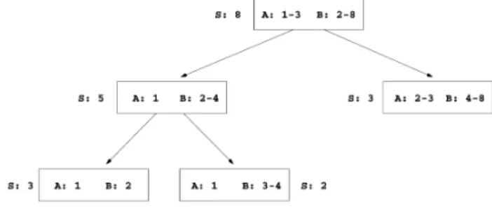
are equal or greater than d_a. In order to find a node in the interval tree, we start from the root and the path taken from each node is defined by the discriminant item, checking whether the item quantity is smaller than the discriminant quantity. An example of an interval tree can be seen in Figure 2. In this figure the itemranges are represented inside the node and the occurrence counter is represented by “S: n”, where n is its value. The discrimi-nant dimension of a node is chosen based on the biggest distance among the items values being inserted and the respective intervals lengths in the rangeset.

Figure 2 – Interval tree for itemset A B

Another property of KD trees that also holds for in-terval trees is that the counters of all leaf nodes are bound to a capacity specified at building time. Thus, whenever the capacity of a node n is reached, an item is chosen as discriminant and the two children of n are created and the rangesets of the children nodes are based on the dis-criminant. As a consequence, the format of the interval tree is a function of the frequency distributions of the various items and their discriminants.

3 Improving Apriori

In this section we describe how quantitative rules are used for making the generation of association rules more efficient. More specifically, we make the candidate prun-ing phase more efficient by reducprun-ing the number of can-didates that are generated to further verification.

The original Apriori approach prunes a candidate itemset C of size k whenever any of its subsets of size k-1 are not frequent (lines 1..4 of the algorithm in Figure 4). Although this approach is safe in the sense that no large itemsets are mistakenly discarded, it is still possible to generate candidates that later show to be not frequent, because the overlap among the transactions accounted in the k-1 itemsets is not large enough for guaranteeing the support to C.

1. A 1 B 1 C 3 D 4

2. A 2 B 1 C 2 - -

3. A 3 B 2 - - D 4

5. A 2 B 1 - - - -

6. A 3 B 2 C 3 - -

7. A 4 - - - - D 4

8. - - B 2 C 1 D 3

9. - - B 4 C 3 - -

10. - - B 1 - - D 1

Figure 3 – Example of a Transaction Database

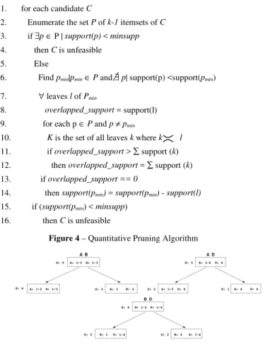
Our strategy, as mentioned, is to use quantitative in-formation to estimate more precisely this overlap in terms of transactions. For instance, if we consider the transac-tion database from Figure 3 and a support threshold of 3, we find five frequent 2-itemsets AB, AC, AD, BC, and BD, with supports 6, 4, 3, 6, and 4, respectively. The original Apriori approach generates two candidate itemsets, A B C and A B D, but the verification in the transaction database reveals that only A B C is frequent. If we verify the interval trees for A B, A D, and B D in Figure 5, we are able to discover that A B D is unfeasible before the counting phase, as follows. The interval (A:4 D:4) does not match any interval in the tree for A B, since there is no node where A is associated with the quantity 4. Thus, the transactions accounted in A D are not all accounted in A B, as we can see in Figure 3, where transaction 7 does not include B. In this case we say that A B D is unfeasible with respect to A D.

We developed an algorithm that generalizes this pro-cedure and enhances significantly the pruning process. There are two basic issues in implementing the strategy described: (1) how to order intervals for sake of compari-son, (2) how to test the overlap among them.

We choose intervals based on a greedy strategy. Since our goal is to prune a candidate k-itemset as early as possible, we focus on the (k-1)-itemset with the smallest support, which presumably is the easiest to be considered unfeasible. We start by checking leaves that have the smallest ranges in all dimensions, which we call rangeset coverage.

We define that two rangesets overlap ( ) when any of their itemranges overlap. More specifically, given two rangesets R = r1, r2,...,rn and S = s1,s2,...,sm, where ri (and

sj) are itemranges We say that R S if ∃r, s|r ∈ R, s ∈ S,

ra = as, ri <= sh V sj <= rh.

The starting point of the algorithm presented in Figure 4 represents the original prune approach, where a candi-date itemset C is unfeasible if any of its subsets of size k-1 are not frequent (lines 2..4). The second phase ex-plores the quantitative information present in the interval trees (lines 5..16). The first step of our prune approach finds the k-1 subset (pmin) with the smallest support value

(line 6) for further evaluation in the intervals trees of all other k-1 subsets. This evaluation takes into account all

interval nodes l from pmin(line 7). The initial overlapped_

support is the support for l itself. We then verify whether this support is valid across all k-1 subsets. Notice that at this level our algorithm is also greedy, since we start with the subset with minimum support and verify whether it holds for all subsets. Thus, for each node considered, the algorithm determines which leaves (k) in the remaining interval trees overlap with the leaves in the interval tree associated with pmin(line 10). We then update overlapped

support if the sum of the supports for all k is smaller than its current value (lines 11..12). We should emphasize that this sum of supports is an upper bound on the support that 1 may have in p and, if it the bound is smaller than the current overall support, then it becomes the new support for that itemrange. If, after verifying all nodes, the resul-tant overlapped_support is 0, the overall support for pmin

is decremented by the support of l (lines 13..14), meaning that l comprises an itemrange that is not present in all subsets needed for the new candidate. Finally, if the sup-port for pmin after the feasibility verifications is smaller

than minsupp then C is assigned as unfeasible (lines 15..16).

1. for each candidate C

2. Enumerate the set P of k-1 itemsets of C

3. if ∃p∈ P | support(p) < minsupp

4. then C is unfeasible

5. Else

6. Find pmin|pmin∈P and ∃p| support(p) <support(pmin)

7. ∀ leaves l of Pmin

8. overlapped_support = support(l)

9. for each p ∈P and p≠pmin

10. K is the set of all leaves k where k l

11. if overlapped_support > ∑ support (k)

12. then overlapped_support = ∑ support (k)

13. if overlapped_support == 0

14. then support(pmin) = support(pmin) - support(l)

15. if (support(pmin) < minsupp)

16. then C is unfeasible

Figure 4 – Quantitative Pruning Algorithm

4 Experimental Results

4.1 Experiments with Synthetic Data

In order to evaluate the efficiency of our algorithm in pruning the candidate sets, we executed the algorithm on transaction databases generated synthetically, which simulate real workloads. The generator of workload takes into account correlations among items acquired by the same customer, that is, the probability of the occurrence of frequent itemsets which may assume four possible distributions: (1) normal (nor), (2) bimodal (bim), (3) exponential (exp), and (4) random (ran). The transaction sizes varied from 10 to 52 items, and the average size of the largest potentially frequent itemset is 10. To create a workload, our generator program takes five parameters: T - number of transactions, M - average size of transac-tions, L - average size of the maximal large itemsets, I - number of items, and D - distribution of occurrences of large itemsets.

Our evaluation is based on two sets of workloads. The first (w-trans) contains workloads with varying number of transactions (from 10000 to 50000) and fixed number of itens (500), aiming to quantify the scalability of the algorithm, while the second set (w-items) comprises workloads with varying number of itens (from 500 to 2500) and fixed number of transactions (50000), as a measure of the complexity of the workload. The remain-ing parameters for both sets of workloads are as follows: the average size of transactions varied from 30 to 40; the average size of the maximal large itemsets is 10; and all four distributions of occurrences aforementioned.

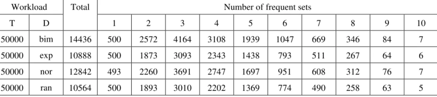
We evaluate our pruning algorithm by considering the number of frequent itemsets in each iteration, the number of candidate itemsets (with and without pruning) and the hit ratio between candidate itemsets and frequent item-sets. We also evaluated the elapsed computational time for executing the algorithm under different workloads and compared execution times that employed or not our pruning strategy. We illustrate these metrics by analyzing the results from four workloads (T=50000, I=500, M=30, L=10, and D = {bim, exp, nor, ran}), considering a 10% support. The number of frequent itemsets at the end of each iteration for these workloads and support are shown in Table 1.

We start our evaluation by verifying the number of candidate itemsets generated during the execution of the algorithm. These data are shown in Table 2, where we can see that our pruning algorithm reduced the overall number of candidate itemsets by up to 16%. In fact, if we consider just the itemsets greater than 2, which are effec-tively pruned, the gains are over 20% for some work-loads.

Workload

T D

Pruning No Pruning Gain

50000 bim 18081 21559 16.13%

50000 exp 14697 16194 9.24%

50000 nor 15996 19082 16.17%

50000 ran 14191 15623 9.17%

Table 2 - Total number of candidate itemset

The effectiveness of our algorithm increases with the size of the itemsets being pruned, as we can see in Table 3, where we compare the number of candidate itemsets per iteration of the algorithm. We can see that our ap-proach reduces the number of itemsets by up 30%. Fur-thermore, our pruning algorithm detected, in some cases, that all unfeasible candidate itemsets, reducing the overall number of iterations (e.g., 10-itemsets in the exponential and in the random workload).

We also evaluated the “hit ratio” of our algorithm, that is the ratio between the number of frequent itemsets and the number of candidate itemsets found by our prun-ing algorithm. We can see in Table 4 that the hit ratio for itemsets greater than 2 is above 64% in all cases, reach-ing 100% in some cases. For instance, in both the expo-nential and random workloads, the pruning algorithm identified as candidates exactly the frequent 10-itemsets.

Table 5 shows the elapsed time for generating rules using the workload described. We can see that our prun-ing algorithm enhances the performance of Apriori in all cases, ranging from 16.5% to 23.9%, providing an aver-age improvement of 21.2%. We should notice that the pruning operations never increased the execution time of the algorithm. In fact, our measurements show that these operations represent a very small fraction of the overall execution time (which is dominated by itemset counting), being limited to few seconds per execution.

Workload

T D

Pruning No Pruning Gain

50000 bim 30405.8 39958.7 23.91%

50000 exp 22376.5 28240.7 20.77%

50000 nor 26865.4 35106.6 23.48%

50000 ran 23416.1 28113.4 16.71%

Workload Number of frequent sets

T D Total

1 2 3 4 5 6 7 8 9 10

50000 bim 14436 500 2572 4164 3108 1939 1047 669 346 84 7

50000 exp 10888 500 1873 3093 2343 1438 793 511 267 64 6

50000 nor 12842 493 2260 3691 2747 1697 951 608 312 76 7

50000 ran 10564 500 1893 3010 2202 1369 774 490 258 63 5

Table 1 – Frequent sets in the Workload

Workload Candidates per itemset size

T D

Prune Total

1 2 3 4 5 6 7 8 9 10

50000 bin Y 18081 500 3976 5055 3764 2288 1247 753 396 94 8

50000 bin N 21559 500 3976 6354 4688 2896 1531 971 510 123 10

50000 exp Y 14697 500 2896 4182 3122 1930 1009 637 335 80 6

50000 exp N 16194 500 2896 4719 3534 2147 1160 742 393 94 9

50000 nor Y 15996 500 3432 4448 3299 1992 1154 705 372 86 8

50000 nor N 19082 500 3432 5591 4108 2522 1417 910 479 113 10

50000 ran Y 14191 500 2892 3928 2972 1858 996 630 327 83 5

50000 ran N 15623 500 2892 4433 3364 2067 1146 734 383 97 7

Table 3 – Number of candidates per itemset size

Workload Hit Ratio per itemset size %

T D Hit Ratio

1 2 3 4 5 6 7 8 9 10

50000 bin 74.75 98.58 48.14 79.49 79.91 82.62 78.65 84.05 80.77 86.84 85.71

50000 exp 65.02 100.00 45.41 78.60 78.89 82.00 80.90 87.44 85.55 88.10 100.00

50000 nor 75.44 100.00 47.23 69.50 65.03 64.28 71.32 71.43 73.26 68.25 85.71

50000 ran 65.67 100.00 45.38 64.79 66.75 65.79 72.76 75.34 74.53 75.00 100.00

Table 4 – Pruning Hit Ratio for Synthetic Workloads

4.2 Mining Web Logs

In order to confirm the performance trends we ob-served using synthetic data, we experimented with a real-life dataset: a web log database obtained from an actual virtual bookstore. We present the results of these experi-ments in this section.

The data consist of the set of requests to a virtual bookstore over an one-week period. We group the re-quests into sessions, so that each session comprises all requests (that is, services such as browse, search, and

pay) for a given user and its frequency, which is its num-ber of occurrences. For sake of applying the quantitative Apriori algorithm, each session becomes a transaction and the resultant rules are common user behaviors that may be used for workload characterization and personal-ization. The size of the web log is 6 MB and there is a total of 153 items, representing different requests, and 35887 sessions with an average size of 15.

from 48.1% in the worst case (1-itemsets) and 91.7% in the best case (3-itemsets). Notice that the gains are simi-lar to those observed in synthetic workloads.

4.3 Algorithm Scalability

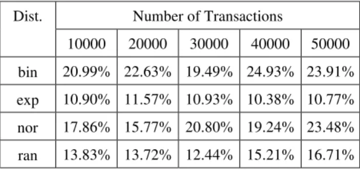
As described previously, we evaluate the scalability of our algorithm through two sets of workloads (w_trans and w_ items). Table 6 shows the performance gains (the ratio between the overall execution times of the quantita-tive Apriori algorithms employing or not our pruning strategy) for workloads comprising from 10000 to 50000 transactions. We can observe that the gain usually in-creases with the number of transactions, however, there are some exceptions as a consequence of the remaining workload parameters being the same in all cases.

Number of Transactions Dist.

10000 20000 30000 40000 50000

bin 20.99% 22.63% 19.49% 24.93% 23.91%

exp 10.90% 11.57% 10.93% 10.38% 10.77%

nor 17.86% 15.77% 20.80% 19.24% 23.48%

ran 13.83% 13.72% 12.44% 15.21% 16.71%

Table 6 – Time Gain for Generating Rules (w_trans)

Table 7 show the gains, in terms of execution times, for varying number of items per transaction. Again, the gain usually increases with the number of items in the transaction. We can explain this trend by the fact that the support is the same for all experiments, and a larger number of items means that each item is less frequent on average.

Number of Items Dist.

500 1000 1500 2000 2500

bin 23.91% 25.63% 29.49% 32.93% 35.91%

exp 10.77% 14.57% 17.99% 19.98% 21.07%

nor 23.48% 25.75% 28.30% 32.14% 34.52%

ran 16.71% 19.27% 22.11% 25.01% 28.91%

Table 7 – Time Gain for Generating Rules (w_items)

5 Related Work

There are several proposals for mining association rules from transaction data. Some of these proposals are constraint-based in the sense that all rules must fulfill a predefined set of conditions, such as support and confi-dence [1,3,7]. The second class identify just the most

interesting rules (or optimal) in accordance to some inter-estingness metric, including confidence, support, gain, chi-squared value, gini, entropy gain, laplace, lift, and conviction [17,6,11]. However, the main goal common to all of these algorithms is to reduce the number of gener-ated rules. We extend the first group of techniques since we do not relax any set of conditions nor employ a inter-estingness criteria to sort the generated rules.

In this context, many algorithms for efficient genera-tion of frequent itemsets have been proposed in the litera-ture since the problem was first introduced in [2]. The DHP algorithm [13] uses a hash table in pass k to perform efficient pruning of (k+1)-itemsets. The Partition algo-rithm [15] minimizes I/O by scanning the database only twice. In the first pass it generates the set of all poten-tially frequent itemsets, and in the second pass the sup-port for all these is measured. The above algorithm are all specialized techniques which do not use any database operations. Algorithms using only general purpose DBMS systems and relational algebra operations have also been proposed [9.10].

There are some other efforts that exploit quantitative information present in transactions for generating asso-ciation rules. In [16], the quantitative rules are generated by discretizing the occurrence values of an attribute in fixed-length intervals and applying the standard Apriori algorithm for generating association rules. However, although simple, the rules generated by this approach may not be intuitive, mainly when there are semantic intervals that do not match the partition employed. Other authors [5, 12, 18] proposed novel solutions that mini-mize this problem by considering the distance among item quantities for delimiting the intervals, that is, their “physical”' placement, but not the frequency of occur-rence as a relevance metric. Our quantitative approach was introduced in [14] and a quantitative interestingness metric was also presented.

6 Final Remarks

In this paper we addressed the problem of minimizing the number of candidate sets that are considered while generating association rules. We achieve such reduction by taking into consideration quantitative information that is usually discarded, since traditional association rules focus just on qualitative correlations.

syntheti-cally generated workloads, reducing not only the number of sets generated but also the overall execution time of the algorithm.

Quantitative association rules can be used in several domains where the traditional approach is employed. The unique requirement for such use is to have a semantic connection between the components of the item-value pairs. We will investigate its use on other applications, such as discovering web access patterns on web logs, predicting web users surfing paths and spatial data clus-tering analysis. Future work also includes evaluating the approach on real workloads and extending it to other data mining algorithms, always exploiting the quantitative perspective.

References

[1] R. Agrawal, T. Imielinski, and A. Swami. Database mining: A performance perspective. In IEEE Transactions on Knowlegde and Data Engineering, December 1993.

[2] R. Agrawal, T. Imielinski, and A. Swami. Mining association rules between sets of items in large databases. In Proc. of the ACM SIGMOD Washing-ton, D.C., pages 207-216, May 1993.

[3] R. Agrawal, H. Mannila, R. Srikant, H. Toivonen, and A.Verkamo. Fast discovery of association rules. In Advances in Knowledge Discovery and Data Mining, San Jose, CA, pages 307-328, 1996.

[4] R. Agrawal and R. Srikant. Fast algorithms for mining association rules. In 20th International Conference on Very Large Data Bases, Santiago, Chile, pages 487 - 499, September 1994.

[5] Y.Aumann and Y.Lindell. A statistical theory for

quantitative association rules. In 5th ACM

SIGKDD International Conference on Knowledge, San Diego, CA, pages 261 - 270, August 1999.

[6] R. Bayardo and R. Agrawal. Mining the most in-teresting rules. In 5th ACM SIGKDD International Conference on Knowledge, San Diego, CA, pages 145 - 154, August 1999.

[7] R. Bayardo, R. Agrawal, and D. Gunopulos. Con-straint-based rule mining in large, dense databases. In 15th International Conference on Data Engi-neering, Sydney, Australia, pages 188 - 197, March 1999.

[8] J. Bentley. Multidimensional binary search trees used for associative searching. In Communications

of ACM, 18(9):509 - 517, 1975.

[9]

M. Holsheimer, M. Kersten, H. Mannila, and H. Toivonen. A perspective on databases and data mining. In 1st International Conference on Knowl-edge Discovery and Data Mining, Montreal, Can-ada, pages 150 - 155, August 1995.

[10] M. Houtsma and A. Swami. Set-oriented mining of association rules. Technical Report RJ 9567, IBM Almaden Research Center, San Jose, CA, October 1993.

[11] B.Liu, W. Hsu, and Y. Ma. Pruning and summariz-ing the discovered associations. In 5th ACM SIGKDD International Conference on Knowledge Discovery and Data Mining, San Diego, CA, pages 125 - 134, August 1999.

[12] R. Miller and Y. Yang. Association rules over interval data. In ACM SIGMOD Conference, Tuc-son, Arizona, pages 452 - 461, May 1997.

[13] J. Park, M. Chen, and P. Yu. An effective hash based algorithm for mining associative rules. In ACM SIGMOD Conference, San Jose, CA, pages 175 - 186, May 1995.

[14] B. Pôssas, F. Ruas, W. Meira, and R. Resende. Geração de regras de associação quantitativas. In XIV Brazilian Database Symposium, Florianópolis, SC, pages 317 - 332, September 1999.

[15] A. Savasere, E. Omiecinski, and S. Navathe. An efficient algorithm for mining association rules in large databases. In 2lst International Conference on Very Large Data Bases, Zurich, Switzerland, pages 432 - 444, 1995.

[16] R. Srikant and R. Agrawal. Mining quantitative association rules in large relational tables. In ACM SIGMOD Conference, Montreal, Canada, pages 1 - 12, June 1996.

[17] G. Webb. Opus: An efficient admissible algorithm for unordered search. In Journal of Artificial Intel-ligence Research, 3:43l - 465, 1995.