Braz. J. Phys. vol.39 número1

Effects of dust charge variation on electrostatic waves in dusty plasmas with temperature anisotropy

M.C. de Juli

Centro de R´adio-Astronomia e Astrof´ısica Mackenzie - CRAAM, Universidade Presbiteriana Mackenzie, Rua da Consolac¸˜ao 896, CEP: 01302-907, S˜ao Paulo, SP, Brasil

R.S. Schneider † and L. F. Ziebell1

Instituto de F´ısica, Universidade Federal do Rio Grande do Sul, Caixa Postal 15051, CEP: 91501-970, Porto Alegre, RS, Brasil.

R. Gaelzer

Instituto de F´ısica e Matem´atica, Universidade Federal de Pelotas, Caixa Postal 354 - Campus UFPel, CEP: 96010-900, Pelotas, RS, Brasil

(Received on 14 January, 2009)

We utilize a kinetic approach to the problem of wave propagation in dusty plasmas, taking into account the variation of the charge of the dust particles due to inelastic collisions with electrons and ions. The components of the dielectric tensor are written in terms of a finite and an infinite series, containing all effects of harmonics and Larmor radius. The formulation is quite general and valid for the whole range of frequencies above the plasma frequency of the dust particles, which are assumed motionless. The formulation is employed to the study of electrostatic waves propagating along the direction of the ambient magnetic field, in the case for which ions and electrons are described by bi-Maxwellian distributions. The results obtained in a numerical analysis corroborate previous analysis, about the important role played by the dust charge variation, particularly on the imaginary part of the dispersion relation, and about the very minor role played in the case of electrostatic waves by some additional terms appearing in the components of the dielectric tensor, which are entirely due to the occurrence of the dust charge variation.

Keywords: Electrostatic waves; Kinetic theory; Magnetized dusty plasmas; Dust charge fluctuation; Wave propagation

1. INTRODUCTION

In the development of a proper kinetic formulation for the analysis of wave propagation and damping in a plasma con-taining a population of charged dust particles, it is necessary to take into account the process of charging of the dust grains. However, despite the recognized importance of this effect to the propagation and damping of waves [1, 2], and despite the recognized need of a kinetic formulation including effects due to the dust charging for proper evaluation of the wave damp-ing [3, 4], most of the published literature utilizes fluid theory to describe the dusty plasmas, and only a small fraction of the published papers take into account the collisional charging of the dust particles [5–8].

Motivated by the importance of the use of a proper kinetic formulation for the analysis of wave behavior in dusty plas-mas with dust grains of variable charge, in a recent paper we have developed a very general mathematical formulation, writ-ing the expressions for the components of the dielectric tensor in terms of an infinite and a finite summation, formally incor-porating effects of all cyclotron harmonics and all orders of Larmor radius, keeping effects due to the dust charge varia-tion [9]. The formulavaria-tion developed is very general in terms of frequency range and direction of propagation, and it is ex-pected to be very useful for application to the study of wave propagation in dusty plasmas in a variety of situations. As an example of application, in Ref. [9] we have also included a brief discussion of the particular case of electrostatic waves

†_{In Memoriam}

∗_{Electronic address:[email protected]}

propagating along the direction of the ambient magnetic field, assuming the case of Maxwellian distributions for electrons and ions in the equilibrium, including some results originated from numerical solutions of the dispersion relation.

In the present paper, we resume the use of the formulation developed and presented in Ref. [9], in order to investigate the dispersion relation for electrostatic waves in a dusty plasma, considering the case of bi-Maxwellian distribution functions for ions and electrons. The analysis therefore includes simul-taneously the effects of the presence of dust particles, includ-ing the effect of the dust charge variation, and the effect of the anisotropy in electron and ion temperatures.

2. THE HOMOGENEOUS MAGNETIZED DUSTY PLASMA MODEL AND THE COMPONENTS OF THE DIELECTRIC

TENSOR

The present paper is an application of the general formalism recently appeared in Ref. [9]. Since the formalism is easily available, the whole set of necessary expressions and defini-tions will not be repeated here, for the sake of economy of space. Nevertheless, it may be useful to repeat here a short account of basic features, which will be made in the following paragraphs.

In our general kinetic formulation we consider a plasma in a homogeneous ambient magnetic fieldB₀=B0ez, in the pres-ence of spherical dust grains with constant radiusa and vari-able electric chargeqd. We assume that the electrostatic energy

of the dust particles is much smaller than their kinetic energy, the so-called weakly coupled dusty magneto-plasmas. This condition is not very restrictive, since a large variety of nat-ural and laboratory dusty plasmas can be classified as weakly coupled [10]. The charging of the dust grains is assumed to oc-cur by the capture of plasma electrons and ions during inelastic collisions between these particles and the dust particles. Since the electron thermal speed is much larger than the ion ther-mal speed, the equilibrium dust charge becomes preferentially negative. The cross-section for the charging process of the dust particles is modeled by we expressions derived from the OML theory (orbital motion limited theory) [11, 12].

Although we assume the occurrence of a magnetic field, the model which we use for the dust charging does not take into ac-count the effect of the magnetic field, being valid only for pa-rameters such that the size of the dust particles is much smaller than the electron Larmor radius. This feature is important, since it has been shown that the effect of the magnetic field on the charging of the dust particles can be safely neglected when the size of the dust particles is much smaller than the electron Larmor radius [13, 14].

Moreover, dust particles are assumed to be immobile, and consequently the validity of the proposed model will be re-stricted to waves with frequency much higher than the charac-teristic dust frequencies. In particular we consider the regime in which|Ωd| ≪ωpd<ω, whereωpd andΩdare the plasma

frequency and the cyclotron frequency of the dust particles, re-spectively. This condition therefore excludes the analysis of the modes which can arise from the dust dynamics, as the so-called dust-acoustic wave.

Using this basic framework, we arrive to expressions for the components of the dielectric tensor which can be separated into two kinds of contributions [15, 16]

εi j=εCi j+εNi j. (1)

Repeating here the commentary which has already appeared along with previous presentations of the formalism, the term

εC

i j is formally identical, except for theizcomponents, to the

dielectric tensor of a magnetized homogeneous conventional plasma of electrons and ions, with the resonant denominator modified by the addition of a purely imaginary term which contains the inelastic collision frequency of dust particles with electrons and ions. For the iz components of the dielectric tensor, in addition to the term obtained with the prescription above, there is a term which is proportional to this inelastic

collision frequency. The termεN

i jarises only due to the process

of variation of the charge of the dust particles, and vanishes in the case of a dustless plasma. Although the formal con-tribution due to this kind of term is already recognized in the literature since at least the first years of the past decade, its contribution to numerical analysis of the dispersion is usually neglected. One notices that the form of theεN

i jcomponents is

strongly dependent on the model used to describe the charging process of the dust particles.

Explicit expressions for the componentsεC

i j andεNi j can be

found in Refs. [9, 15, 16]. Particularly, in Ref. [9] the ex-pressions appear according to the formulation and definitions to be used in the present paper. According to this novel formu-lation, the components of the dielectric tensor can be written in terms of a double summation, one finite and another infi-nite, in which the contribution of harmonics and Larmor radius terms is shown explicitly. For the ‘conventional’ contribution, a componentεC

i jcan be written as follows εC

i j=δi j+δizδjzezz+N δiz+δjz

⊥ χi j, (2)

while a componentεN

i jis written as

εNi j=

U

S

In the case of electrostatic waves (ES waves) and parallel propagation, which the subject of the present application, the dispersion relation is simply given byεzz=0. Therefore, we

present here only the explicit expressions for thezz contribu-tions to the dielectric tensor. For general distribucontribu-tions and ar-bitrary directions of propagation, the contribution to the ‘con-ventional’ part appears as follows

χzz= v2_∗ c2

∑

β 1 r2

β

ω2

pβ

Ω2

∗

1 nβ0

∞

∑

m=1

_q

⊥

rβ

2(m−1)

(4)

× m

∑

n=−m

a(|n_|,m_{− |}n_|)

J(n,m,2;f_β0) +iJν(n,m,1;fβ0)

,

ezz=−

1 z2

∑

β

ω2

pβ

Ω2

∗

1 n_β0

Z d3uuk

u_⊥

L

+1 z2

∑

β

ω2

pβ

Ω2

∗

1 n_β0a(0,0)

J(0,0,2;f_β0) +i Jν(0,0,1;fβ0)

,

where

J(n,m,h;f_β0)≡ Z

d3u

z uh_ku_⊥2(m−1)u_⊥L(f_β0) z₋nr_β−q_ku_k+iν˜0

βd

, (6)

Jν(n,m,h;fβ0) = Z

d3u ˜

ν0 βdu

h

ku

2(m−1)

⊥ u⊥

L

βd

, (7)

L=1

γ

γ−q_zku_k

_∂

∂u_⊥+ q_k

z u⊥

∂ ∂u_k

L

∂u_⊥−u⊥

∂ ∂u_k ,

with the dimensionless variables z= ω

Ω_∗, qk,⊥=

k_k,⊥v_∗

Ω_∗ , uk,⊥=

p_k,⊥ m_βv_∗ ,

r_β=Ωβ

Ω_∗, ν˜

0 βd=

ν0 βd(u)

Ω_∗ , u=

u2_k+u2_⊥1/2 ,

where the inelastic collision frequency between plasma parti-cles and dust partiparti-cles is given by

ν0_βd(u) =πa 2_n

d0v∗

u

u2₋2qd0qβ am_βv2

∗

H

u2₋2qd0qβ am_βv2

∗

.

The quantitiesΩ_∗andv_∗are a characteristic frequency and a velocity, respectively, which are considered convenient for normalization in the case of a particular application. For the present application, we use Ω_∗=ω0

pe0 and v∗=cs, where cs= (Te/mi)1/2is the ion-sound velocity andω0_pe0is the

equi-librium electron plasma angular frequency in the absence of dust. The quantityqd0is the equilibrium value of the charge of the dust particles, which we will denote asqd0=−Zd0e.

The contribution of the ‘new’ part, for general distributions and directions of propagation, appears as follows,

U

1

z+i(˜νch+ν˜1)

∑

pβ

Ω2

∗

1 n_β0

∞

∑

m=0 +m

∑

n=−m

_q

⊥

r_β

2m

×a(|n_|,m_{− |}n_|)JU(n,m,1,0;fβ0), (8)

S

∑

ω2

pβ

Ω2

∗

1 n_β0

∞

∑

m=0 +m

∑

n=−m

_q

⊥

r_β

2m

×a(|n_|,m_{− |}n_|)

JνL(n,m,1;fβ0) +i Jνν(n,m;fβ0)

+aΩ∗ 2v_∗

1 z

∑

ω2

pβ

Ω2

∗

1

n_β0Jν0(fβ0), (9)

˜

νch= aΩ_∗

2v_∗

∑

ω2

pβ

Ω2

∗

1

n_β0Jch(fβ0), (10)

˜

ν1=−i aΩ_∗

2v_∗

∑

ω2

pβ

Ω2

∗

1 n_β0

∞

∑

m=0 +m

∑

n=−m

q_⊥ r_β

2m

×a(|n_|,m_{− |}n_|)JU(n,m,0,1;fβ0), (11) where

JU(n,m,h,l;fβ0) =

Z d3u

z(ν˜0

βd/z)lfβ0 z₋nr_β−q_ku_k+iν˜0

βd

(12)

×u h

ku2⊥m

u H

u2+2Zd0eqβ am_βv2

∗

,

JνL(n,m,h;fβ0) =

Z d3u ν˜

0 βduh_ku

2m−1

⊥ L(fβ0) z₋nrβ−qkuk+iν˜0βd

, (13)

Jνν(n,m;fβ0) =

Z d3u

z(˜ν0 βd/z)

2_u2m−1

⊥

L

βd

, (14)

Jν0(fβ0) = Z

d3u ˜

ν0 βd z

L

u_⊥ , (15)

Jch(fβ0) = Z

d3u f_β0 1 uH

u2+2Zd0eqβ am_βv2

∗

, (16)

with ˜ν1=ν1/Ω∗and ˜νch=νch/Ω∗.

For the case of parallel propagation (q_⊥=0), Eqs. (5), (8), and (9), lead to

ezz =−

1 z2

∑

β ω2 pβ Ω2 ∗ 1 n_β0

Z d3u uk

u_⊥

L

+1 z2

∑

β ω2 pβ Ω2 ∗ 1 n_β0

J(0,0,2;f_β0) +i Jν(0,0,1;fβ0)

,

U

1

z+i(˜νch+ν˜1)

∑

pβ

Ω2

∗

1

n_β0JU(0,0,1,0;fβ0),

S

1 z

∑

ω2

pβ

Ω2

∗

1 n_β0

JνL(0,0,1;fβ0) +i Jνν(0,0;fβ0)

+aΩ∗ 2v_∗

1 z

∑

ω2

pβ

Ω2

∗

1 n_β0

Jν0(fβ0),

where, from Eqs. (10) and (11),

˜

νch= aΩ_∗

2v_∗

∑

ω2

pβ

Ω2

∗

1 nβ0

Jch(fβ0),

˜

ν1=−i aΩ_∗

2v_∗

∑

ω2

pβ

Ω2

∗

1 nβ0

JU(0,0,0,1;fβ0).

Further development can be made in the particular case of bi-Maxwellian distributions for ions and electrons,

f_β0(u_k,u_⊥) = nβ0 (2π)3/2_u2

β⊥uβk

e−u2k/(2u2βk)_e−u2⊥/(2u2β⊥)_{. (17)}

For these distributions,

L

u2 β⊥

and

L(f_β0) =− u⊥

γu2_β⊥

γ−q_zku_k 1−∆β

f_β0, (19)

where

∆β= u2_β⊥

u2_βk = T_β⊥

T_βk .

whereu_β⊥=v_β⊥/v_∗andu_βk=v_βk/v_∗, withv_β⊥=qT_β⊥/m_β andv_βk=qT_βk/m_β.

For the case of these distributions and using as an approx-imation the average value of the collision frequency instead of the actual momentum-dependent value, the integrals which are necessary for the components of the dielectric tensor can be evaluated, leading to the following expressions,

J(0,0,2;f_β0) = (√2)2_n β0 u2 βk u2 β⊥ ζ0

βζˆ0β

h

1+ζˆ0 βZ(ζˆ0β)

i

−(1−∆β)

1 2+ (

ˆ

ζ0 β)2

h

1+ζˆ0 βZ(ζˆ0β)

i

,

Jν(0,0,1;fβ0) = ( √

2)2_(1−∆ β)nβ0

×u 2 βk

u2_β⊥ ˜

νβ z ζ

0 βζˆ0β

h

1+ζˆ0_βZ(ζˆ0_β)i ,

JU(0,0,0,1;fβ0)≃ −Γ

1 2

(√2)−1

_ν˜

β z

n_β0

×(u_β⊥)−1(u_βk)0ζ0_βZ(ζˆ0_β),

JU(0,0,1,0;fβ0)≃ −Γ

1 2

(√2)0

_ν˜

β z

0

n_β0

×(u_β⊥)−1(u_βk)1ζ_β0h1+ζˆ0_βZ(ζˆ0_β)i ,

Jνν(0,0;fβ0) =

_ν˜

β z

2

(√2)1 1−∆β

n_β0

×(u_β⊥)−2(u_βk)ζ0_βh1+ζˆ0_βZ(ζˆ0_β)i .

JνL(0,0,1;fβ0) = ˜

νβ

z J(0,0,1;fβ0) = ˜

νβ z (

√ 2)1n_β0

× u_β⊥−2u_βknζ0_βh1+ζˆ0_βZ(ζˆ0_β)i−(1−∆β)ζˆ0β

h

1+ζˆ0_βZ(ζˆ0_β)io,

Jν0(fβ0) =0, where

ˆ

ζn β=

z₋nr_β+iν˜β √

2q_ku_βk , ζ 0 β=

z √

2q_ku_βk,

˜

νi= νi Ω_∗=2(

√

2π)(εni0) c3

Ω3

∗

a2_Ω2

∗

c2 v_∗

c u_ik

∆i

× Z 1

0

dµ ∆i

1+µ2_(∆

i−1)

∆i

1+µ2_(∆

i−1)

+χi_k

,

˜

νe= νe Ω_∗=2(

√

2π)(εni0) c3

Ω3

∗

a2Ω2

∗

c2 v_∗

c ue_k

∆e × Z1 0 dµ _∆ e

1+µ2_(∆

e−1) 2

e−|χek|[1+µ2(∆e−1)]/∆e_.

Moreover, the first integral which contributes toezzbecomes

simply the following

Z d3u uk

u_⊥

L

n_β0 u2_βk u2_β⊥ .

Details of the evaluation can be found in appendix A. Using these results, and using also Eq. (A16) for theJch, the

disper-sion relation becomes

ΛC+ΛN=0, (20)

where

ΛC=1+2 z2

∑

β

ω2

pβ

Ω2

∗

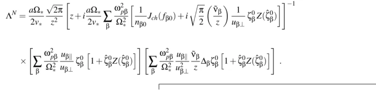
ΛN₌aΩ∗

2v_∗ √

2π

z2

"

z+iaΩ∗ 2v_∗

∑

ω2

pβ

Ω2

∗

1 nβ0

Jch(fβ0) +i

r π

2

_ν˜

β z

1 uβ⊥

ζ0 βZ(ζˆ0β)

#−1

×

"

∑

β

ω2

pβ

Ω2

∗

u_βk u_β⊥ζ

0 β

h

1+ζˆ0_βZ(ζˆ0_β)i

# "

∑

β

ω2

pβ

Ω2

∗

u_βk u2_β⊥ ˜

νβ z ∆βζ

0 β

h

1+ζˆ0_βZ(ζˆ0_β)i

#

.

3. NUMERICAL ANALYSIS

For the numerical analysis we consider parameters which are in the range of parameters of interest for stellar winds: ion temperatureTi=1.0×104K, ion densityni0=1.0×109 cm−3, ion charge number Zi=1.0, and ion mass mi =mp,

wherempis the proton mass, witha=1.0×10−4cm as the

radius of the dust particles. The ion density which has been as-sumed is rather high when compared, for instance, with the so-lar wind plasma, but is reported to occur in outbursts of carbon-rich stars [17].

3.1. Ion-acoustic waves, isotropic Maxwellian distributions

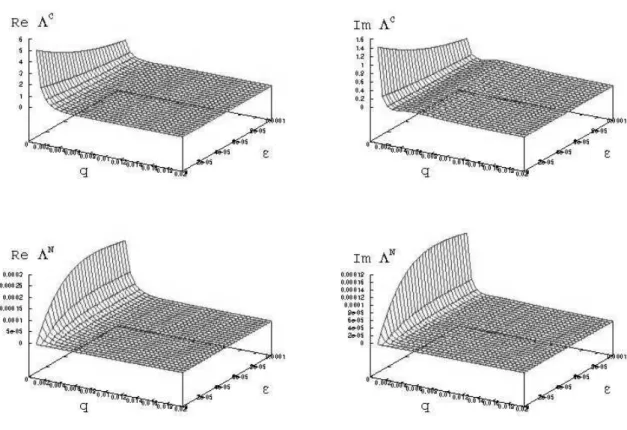
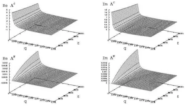
Initially, we estimate the magnitude of the contribution of the ‘new’ terms to the dispersion relation of ES waves, and compare it with the ‘conventional’ contribution, for the case of isotropic Maxwellian distributions. In order to do that we assume the occurrence of weakly damped oscillations with fre-quency in the range of ion-acoustic waves, choosing the values z= (1×10−2_,−2×10−4_{)for the numerical estimation. For} this value ofzand for the parameters considered in the previ-ous paragraph, and assumingTe/Ti=10.0, we plot in Fig. 1

the quantitiesΛC _andΛN_{, namely the ‘conventional’ and the}

‘new’ contributions to the ES dispersion relation, as defined in Eq. (20), versus normalized wave-numberq and normalized dust densityε. The upper panels of Fig. 1 show respectively, from left to right, the real and the imaginary parts ofΛC_{, while}

the bottom panels show from left to right the real and the imag-inary parts ofΛN_{. It is seen that for most of the interval ofq}

andεdepicted in the figure the real and imaginary contribu-tions ofΛN _{are about four orders of magnitude smaller than}

the corresponding contributions ofΛC_{. Similar figures and}

re-sults can be obtained for different values of the ratioTe/Ti, as

in the cases ofTe/Ti=1.0 andTe/Ti=20.0, which appeared

in [9].

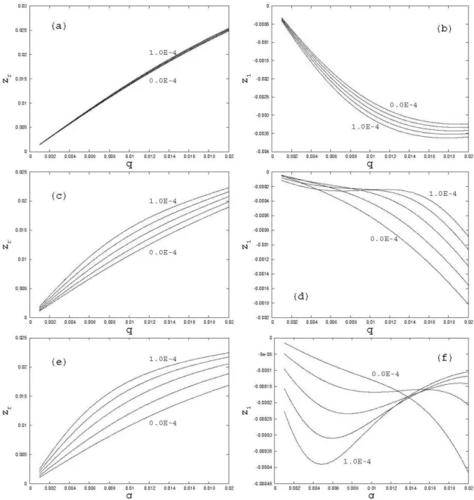
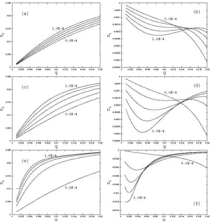
We further explore the role of the dust particles and of the ‘new’ contribution for the dispersion relation of ES waves in the case of isotropic Maxwellian distributions, by numerically solving the expanded form of Eq. (20) for the frequency range of ion-acoustic waves. Fig. 2 shows the value ofzr and the

corresponding values of the imaginary partzi, as a function of qand five values ofε(0.0, 2.5×10−5, 5.0×10−5, 7.5×10−5, and 1.0×10−4), for three values of the temperature ratioTe/Ti

(1, 10, and 20). Figure 2(a) shows that the quantityzr is

rela-tively insensitive to the presence of the dust, forTe=Ti.

Fig-ures 2(c) and 2(e) show that, for increasing values of the ratio Te/Ti, the effect of the dust on the real part of the dispersion

relation becomes more and more pronounced. Regarding the

imaginary part, Figure 2(b) shows that Landau damping occurs for the whole range ofqvalues considered, namely the damp-ing which occurs for absence of dust, ε=0.0, and that the presence of dust increases the damping for the whole range appearing in the figure, forTe=Ti. On the other hand, Fig.

2(d) shows that forTe/Ti=10 the increase of the dust

popula-tion increases the damping in the region of very smallq, and decreases the damping for sufficiently largeq(q_≥0.008, for the parameters utilized). There is an intermediate region for which the presence of the dust population initially contributes to decrease of damping, and then contributes to a renewed in-crease of damping, for sufficiently large ε. Similar features are seen more clearly with the increase of the ratioTe/Ti.

Fig-ure 2(f) shows that for smallqthe damping is appreciably in-creased with the increase ofε, while forq_≥0.015 the damping is clearly decreased by the increase in the dust population.

The explanation for this behavior of the imaginary partziis

as follows. The basic feature to be considered is that the pres-ence of dust lead to two competitive effects. One of the effects is the damping due to the dust charge variation, depending on the frequency of inelastic collisions on the denominator of the velocity integrals appearing in the dielectric tensor. Another effect is the reduction in the electron population, due to the capture of electrons by the dust particles, which contribute to reduction of electron Landau damping. For Te/Ti=1.0 the

electron Landau damping is meaningful for large q, and de-creases for small q, because the resonant velocity becomes much larger than the electron thermal velocity. The dust charge variation constitutes an additional damping mechanism. This effect dominates over the decrease of Landau damping because the capture of electrons is not very significant forTe/Ti=1.0.

Figure 3 shows that forTe/Ti=1.0 andε=1.0×10−4the

elec-tron density is still more than 80 % of the population in a dust-less plasma. The consequence is that the damping is increased by the process of dust charge variation, for the whole range ofq, with the increase of the dust density. ForTe/Ti=10.0,

on the other hand, electron Landau damping is significant for the higher end of the q range considered, but less important for smallq, if compared with the case ofTe/Ti=1.0. With

the increase in the dust population, the damping is enhanced for smallq, since in the region of small Landau damping the damping due to the dust charge variation is dominant. This possibility of damping due to collisional charging has already been noticed by other authors [3, 18]. In the higher end of theqregion, however, Landau damping is sufficiently high to become dominant. Although the presence of dust introduces damping due to the dust charge variation, the dominant effect is the reduction of Landau damping due to the reduction of the electron population. Figure 3 shows that forTe/Ti=10.0 the

features are even more evident forTe/Ti=20.0. For smallq

the Landau damping is negligible in this case. With the in-crease of the dust population, there is enhancement of damping for smallq, due to the mechanism of dust charge variation. For the higher end of theqregion, however, the damping due to the dust charge variation is overcome by Landau damping. With the increase of the dust populationε, the electron population is severely reduced, as shown by Fig. 3, and the overall effect is the reduction of the wave damping shown by Fig. 2(f).

We point out that in Fig. 2 we have plotted the results ob-tained with the dispersion relation given by Eq. (20). We have also plotted in the same figure the results obtained from a dis-persion relation given byΛC _{=0, obtained by neglecting the}

‘new’ contribution to the dielectric tensor. The results hardly can be distinguished in the scale of the figure, reflecting the fact that for the range of frequency and for the parameters uti-lized the effect of the ‘new’ contribution is negligible in the dispersion relation of ES waves. In a color version of Fig. 2, using blue color for the results obtained with the full dispersion relation and red color for the results obtained considering only the “conventional” contribution to the dispersion relation, the two different results appear so close that the curves feature a light purple color, result of the superposition of the results fea-tured with blue color and the results feafea-tured with red color. In a monochromatic version of Fig. 2, using two different line styles, the two different results can hardly be distinguished.

3.2. Ion-acoustic waves, bi-Maxwellian distributions

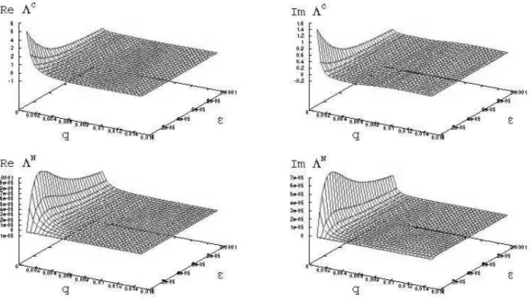
At this point we proceed to the estimation of the magnitude of the contribution of the ‘new’ terms to the dispersion relation of ES waves in anisotropic plasmas, and compare it with the ‘conventional’ contribution. In order to do that we again as-sume the occurrence of weakly damped oscillations with fre-quency in the range of the ion-acoustic waves, assuming a typ-ical normalized frequencyz= (1.0×10−2,−2×10−4). For this value ofzand for the parameters considered in the previ-ous paragraph, and assumingTe/Ti=1.0, and considering the

case ofTe_⊥/Tek=0.1 andTi_⊥/Tik=0.1, we plot in Fig. 4 the

quantitiesΛC _andΛN _{versus normalized wave-number qand}

normalized dust densityε. The upper panels of Fig. 4 show respectively, from left to right, the real and the imaginary parts ofΛC_{, while the bottom panels show from left to right the real}

and the imaginary parts ofΛN_{. It is seen that for most of the}

interval ofqandεdepicted in the figure the real and imaginary contributions ofΛN _{are much smaller than the corresponding}

contributions of ΛC_{, similarly to what occurs in the case of}

isotropic Maxwellian distributions.

In Fig. 5 we show the same quantities depicted in Fig. 4, for the case ofTe_⊥/Tek=10.0 andTi_⊥/Tik=10.0, with the other

parameters all equal to those used for Fig. 1. The comments which can be made about Fig. 5 are similar to those made about Fig. 4, and also similar to those made about Fig. 1, which was obtained for the case of isotropy of temperatures.

Figures 4 and 5 have been obtained assuming equal ion and electron temperatures. In the case of electron temper-ature larger than ion tempertemper-ature, similar results can be ob-tained. The only point to be observed is that, for increasing ratio of perpendicular and parallel temperatures, the magni-tudes ofΛC _andΛN _{at smallq, which are seen to grow with}

εin the range depicted in Figs. 4 and 5, are seen to decrease again at sufficiently largeε. This feature is illustrated in Figs. 6 and 7, which show the same quantities appearing in Figs. 4 and 5, forTe/Ti=4.0 andTe/Ti=10.0, respectively, with Te⊥/Tek=10.0 andTi⊥/Tik=10.0, and the other parameters

all equal to those used for Fig. 1. The opposite side of the anisotropy range is illustrated by Fig. 8, which shows the case ofTe/Ti=10.0, withTe_⊥/Tek=0.1 andTi_⊥/Tik=0.1, and the

other parameters all equal to those used for Fig. 1.

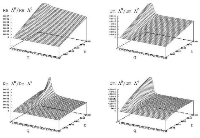
Both in the case of∆β=0.1, shown in Fig. 4, in the case of

∆β=10.0, shown in Figs. 5 and 6, and in the case of∆β=1.0, illustrated in Fig. 1, the comparison between the magnitude of the ‘conventional’ and ‘new’ contribution becomes more dif-ficult in the region of the graphics where these contributions both approach zero. In order to improve the accuracy of obser-vation, we show in Fig. 9 the ratio between the ‘new’ and the ‘conventional’ contributions, for one of the cases discussed. In the upper line of Fig. 9 we show at the left-hand side the ratio between the real parts of the contributions, and in the right-hand side the ratio between the imaginary parts, for the case Te⊥/Tek=0.1 andTi⊥/Tik=0.1, withTe/Ti=1.0, and other

parameters as in Fig. 1. At the bottom line, we show the cor-responding figures for the case of perpendicular temperatures much above parallel temperatures, withTe_⊥/Tek=10.0 and

Ti_⊥/Tik=10.0, withTe/Ti=1.0, and other parameters as in

Fig. 1.

The conclusion to be drawn from Fig. 1, for the case of plas-mas with isotropy of temperature, and from Figs. 4, 5, 6, and 9 is that, although the dust population may introduce significant contribution to the dispersion relation of electrostatic waves in the range of frequencies characteristics of ion-acoustic waves, this contribution is mostly due to the ‘conventional’ part of the dielectric tensor. At least for the parameter regime which has been investigated, the ‘new’ contribution is shown to give only a negligible contribution to the dispersion relation.

We continue with the investigation of the role played by the dust particles and by the ‘new’ contribution for the dispersion relation of ES waves in anisotropic plasmas, by discussing the numerical solution of the dispersion relation. In Fig. 10 we consider the solution corresponding to ion-acoustic waves, also for three situations of temperature anisotropy. Fig. 10(a) shows the value ofzrfor ion-acoustic waves, as a function of qzand five values ofε(0.0, 2.5×10−5, 5.0×10−5, 7.5×10−5,

and 1.0×10−4), for Te=Ti and perpendicular temperature

much smaller than parallel temperature (Te⊥/Tek=Ti⊥/Tik=

0.1), with other parameters as in Fig. 1. Figure 10(b) shows the corresponding values of the imaginary part of the normalized frequency,zi. It is is seen that the presence of the dust

pop-ulation modifies very significantly the imaginary partzi. The

damping, measured by the absolute value ofzi, is enhanced for

smallqz, due to the presence of the dust, but can be

apprecia-bly reduced for largerqz, also due to the presence of the dust.

For the real partzr, Fig. 10(c) shows that the effect of the dust

is not very significant, although not negligible.

The case of perpendicular temperature larger than the paral-lel temperature is seen in Figs. 10(e) and 10(f), at the bottom line of Fig. 10. Figure 10(e) shows the value ofzr for

ion-acoustic waves, as a function ofqz and five values ofε(0.0,

2.5×10−5, 5.0×10−5, 7.5×10−5, and 1.0×10−4), forTe=Ti

andTe⊥/Tek=Ti⊥/Tik=10.0, with other parameters as in Fig.

FIG. 1: (upper left) Real part of the “conventional” contribution to the dispersion relation, vs. qandε=nd/ni0; (upper right) imaginary part of the “conventional” contribution; (bottom left) Real part of the “new” contribution; (bottom right) imaginary part of the “new” contribution; z= (1.0×10−2,−2.0×10−4), in the range of ion-acoustic waves. Isotropic Maxwellian distributions for ions and electrons, withTi=1.0×104 K andTe/Ti=10. Other parameters:ni0=1.0×109cm−3,Zi=1.0,mi=mp, wherempis the proton mass, anda=1.0×10−4cm.

temperature the real part of the normalized frequency is much more affected by the presence of the dust than in the case of smaller perpendicular temperature. The imaginary partzi is

also affected significantly by the presence of the dust popula-tion, as shown by Fig. 10(f). Qualitatively, it is seen that the effect is similar to that occurring in the case of perpendicular temperature smaller than parallel shown in Fig. 10(b), in the sense that the damping, measured by the absolute value ofzi, is

enhanced for smallqz, due to the presence of the dust, but can

be appreciably reduced for largerqz, also due to the presence

of the dust.

The middle line of Fig. 10 shows the case of isotropy of temperatures, in between the cases depicted at the top line and at the bottom line. Figures 10(c) and 10(d) show the values of zrandzi, respectively, for ion-acoustic waves, as a function of qzand five values ofε(0.0, 2.5×10−5, 5.0×10−5, 7.5×10−5,

and 1.0×10−4), forTe=TiandTe⊥/Te_k=Ti⊥/Ti_k=1.0, with

other parameters as in Fig. 1.

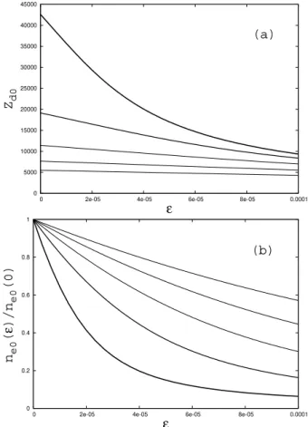
Additional information may be obtained by considering the dependence of the electron density and of the equilibrium value of the charge of the dust particles, as a function of the dust density. In Fig. 11 we show the values of the dust charge Zd0and of the electron densityne0as a function ofε, for five values of the ratioT_⊥/T_k, consideringT_ek=20T_ik, for fixed ion density, for the case of ion-sound waves. It is seen that forT_⊥=0.2T_kthe value ofZd0reduced by nearly 30 % when

εis changed between 0.0 and 1.0×10−4, while it is reduced in the same range to nearly 15 % of the original value in the case ofT_⊥=5.0T_k. It is also seen that the value ofne0changes

by approximately 60 % whenεis changed between 0.0 and 1.0×10−4, in the case ofT_⊥/T_k=0.2, and is reduced to al-most 5 % of the original value in the caseT_⊥/T_k=5.0.

The dependence ofZd0andne0on the ratio of electron and ion temperatures, for anisotropic situations, is illustrated in Fig. 12. Figure 12(a) shows the values ofZd0as a function ofε, for four values of the ratioT_ek/T_ik, for a case with anisotropy of temperatures, withT_⊥/T_k=5.0. Figure 12(b) shows the values of the ratione0(ε)/ne0(0), as a function of ε, for four

values of the ratioTe_k/Ti_k, forT⊥/Tk=5.0. It is seen that the

density of electrons decrease with the increase ofε, substan-tially faster for the case of high values of the ratioT_ek/T_ikthan for the case in which this ratio is equal to the unity.

3.3. Langmuir waves, bi-Maxwellian distributions

We proceed by estimating the magnitude of the contribution of the ‘new’ terms to the dispersion relation of ES waves in anisotropic plasmas, now considering the case of waves with frequency in the range of the Langmuir waves, assuming a typ-ical normalized frequency z= (1.1×100,−1×10−3). For this value ofzand for the parameters considered in the pre-vious paragraph, and assumingTe/Ti=1.0, and considering

the case ofT_e⊥/T_ek=0.1 andT_i⊥/T_ik=0.1, we plot in Fig. 13 the quantitiesΛC _andΛN_{, namely the ‘conventional’ and the}

FIG. 2: Real and imaginary parts of the normalized frequency (zrandzi) obtained from the dispersion relation for ion-acoustic waves in the case of isotropic Maxwellian distributions for ions and electrons, vs. q, for several values ofε=nd/ni0(0.0, 2.5×10−5, 5.0×10−5, 7.5×10−5, and 1.0×10−4); (a)zr, withTe/Ti=1.0; (b)zi, withTe/Ti=1.0; (c)zr, withTe/Ti=10.0; (d)zi, withTe/Ti=10.0; (e)zr, withTe/Ti=20.0; (f)zi, withTe/Ti=20.0; other parameters the same as used to obtain Fig. 1.

from left to right, the real and the imaginary parts ofΛC_{, while}

the bottom panels show from left to right the real and the imag-inary parts ofΛN_{. It is seen that for most of the interval ofq}

andεdepicted in the figure the real and imaginary contribu-tions ofΛN _{are several orders of magnitude smaller than the}

corresponding contributions ofΛC_.

In Fig. 14 we show the same quantities depicted in Fig. 13, for the case of T_e⊥/T_ek=10.0 and T_i⊥/T_ik=10.0, with the other parameters all equal to those used for Fig. 13. The com-ments which can be made about Fig. 14 are similar to those made about Fig. 13, and also similar to those made about Fig. 1 of Ref. [9], where the case of isotropic temperatures has

been discussed. The conclusion is that the dust population may introduce significant contribution to the dispersion relation of electrostatic waves in the range of frequencies characteristics of Langmuir waves, but this contribution is mostly due to the ‘conventional’ part of the dielectric tensor. At least for the parameter regime which has been investigated, the ‘new’ con-tribution is shown to give only a negligible concon-tribution to the dispersion relation.

In Fig. 15 we consider the solution corresponding to Lang-muir waves, for three situations of temperature anisotropy. Fig. 15(a) shows the value ofzr as a function ofqzand five values

0 0.2 0.4 0.6 0.8 1

0 2e-05 4e-05 6e-05 8e-05 0.0001

ne0

(

ε

)/n

e0

(0)

ε

T_e/T_i=1.0

T_e/T_i=10.0

T_e/T_i=20.0

FIG. 3: Ratio between the electron density in a dusty plasma and the equilibrium electron density in the absence of dust, vs. ε=nd/ni0, for three values of the ratioTe/Ti, in the case of isotropic Maxwellian distributions for ions and electrons, Other parameters the same as used to obtain Fig. 1.

FIG. 4: (upper left) Real part of the ‘conventional’ contribution to the dispersion relation, vs. qandε=nd/ni0; (upper right) imaginary part of the ‘conventional’ contribution; (bottom left) Real part of the ‘new’ contribution; (bottom right) imaginary part of the ‘new’ contribution; Te=Ti,∆β=Tβ⊥/Tβk=0.1, forβ=i,e, andz= (1.0×10−2,−2.0×10−4), in the range of ion-acoustic waves. Other parameters the same as used to obtain Fig. 1.

forTe=Ti and perpendicular temperature much smaller than

parallel temperature (Te⊥/Te_k=Ti⊥/Ti_k=0.1), with other

pa-rameters as in Fig. 13. Figure 15(b) shows the corresponding values of the imaginary part of the normalized frequency,zi. It

is is seen that the presence of the dust population do not mod-ifies appreciably the root of the dispersion relation, either the

real or the imaginary part.

Figure 15(e) shows the value of zr for Langmuir waves,

as a function of qz and five values of ε (0.0, 2.5×10−5,

5.0×10−5, 7.5×10−5, and 1.0×10−4), forTe=Ti and

FIG. 5: (upper left) Real part of the ‘conventional’ contribution to the dispersion relation, vs. qandε=nd/ni0; (upper right) imaginary part of the ‘conventional’ contribution; (bottom left) Real part of the ‘new’ contribution; (bottom right) imaginary part of the ‘new’ contribution; Te=Ti,∆β=Tβ⊥/Tβk=10.0, forβ=i,e, andz= (1.0×10−2,−2.0×10−4), in the range of ion-acoustic waves. Other parameters the same as used to obtain Fig. 1.

13. Figure 15(e) shows that in this case of larger perpendic-ular temperature the real part of the normalized frequency is much more affected by the presence of the dust than in the case of smaller perpendicular temperature. Particularly in the region of small wave-number (small qz), the value ofzr can

be reduced by a factor which goes up to almost 50%, for dust population rising between the caseε=0.0 and the case

ε=1.0×10−4. Figure 15(f) shows the corresponding values of the imaginary part of the normalized frequency, zi.

Con-trarily to what happens in the case in which the perpendicular temperature is smaller than the parallel temperature, shown in Fig. 15(b), Fig. 15(f) shows that in the case of larger perpen-dicular temperature the value of the imaginary partzi can be

very appreciably affected by the presence of the dust popula-tion. For a given value of the normalized wave numberqz, the

magnitude of the imaginary part ofziis significantly increased

by the presence of the dust.

In between the cases shown at the top line and at the bot-tom line of Fig. 15, we consider the case of equal parallel and perpendicular temperatures. Figure 15(c) shows the value of zrfor Langmuir waves, as a function ofqzand five values ofε

(0.0, 2.5×10−5, 5.0×10−5, 7.5×10−5, and 1.0×10−4), for Te=Ti and perpendicular temperature equal to parallel

tem-perature (Te⊥/Te_k=Ti⊥/Ti_k=1.0), with other parameters as

in Fig. 13. Figure 15(d) shows the corresponding values of the imaginary part of the normalized frequency,zi.

Let us now consider the dependence of the electron density and of the equilibrium value of the charge of the dust particles, as a function of the dust density. In Fig. 16 we show the val-ues of the dust chargeZd0 and of the electron densityne0as a function ofε, for five values of the ratioT_⊥/T_k, considering Te_k=Ti_k, for fixed ion density. The case ofTe_k=Ti_kis the

case relevant for Langmuir waves. It is seen that the value of Zd0is basically independent ofεin the range considered, for T_⊥<T_k, changing by less than 5 % whenεis changed between 0.0 and 1.0×10−4, in the caseT_⊥=T_k. For larger values of this ratio the value ofZd0becomes more dependent onε, al-though even forT_⊥/T_k=5.0 the change obtained is only of order of 20 %, in the range considered. It is also seen that the value ofne0changes by approximately 8 % whenεis changed between 0.0 and 1.0×10−4, in the case ofT_⊥/T_k=0.2, and is reduced to almost 50 % of the original value in the case T_⊥/T_k=5.0. These results show that the electron density and the dust charge are more and more sensitive to the dust density for increasing values of the ratioT_⊥/T_k, for fixed ion density.

4. CONCLUSIONS

direc-FIG. 6: (upper left) Real part of the ‘conventional’ contribution to the dispersion relation, vs. qandε=nd/ni0; (upper right) imaginary part of the ‘conventional’ contribution; (bottom left) Real part of the ‘new’ contribution; (bottom right) imaginary part of the ‘new’ contribution; Te/Ti=4.0,∆β=Tβ⊥/Tβk=10.0, forβ=i,e, andz= (1.0×10−2,−2.0×10−4), in the range of ion-acoustic waves. Other parameters the same as used to obtain Fig. 1.

FIG. 7: (upper left) Real part of the ‘conventional’ contribution to the dispersion relation, vs. qandε=nd/ni0; (upper right) imaginary part of the ‘conventional’ contribution; (bottom left) Real part of the ‘new’ contribution; (bottom right) imaginary part of the ‘new’ contribution; Te/Ti=10.0,∆β=Tβ⊥/Tβk=10.0, forβ=i,e, andz= (1.0×10−2,−2.0×10−4), in the range of ion-acoustic waves. Other parameters the same as used to obtain Fig. 1.

tion of the ambient magnetic field. The most important motiva-tion was the investigamotiva-tion of the effect of some contribumotiva-tions to the dielectric tensor which usually appear in theoretical analy-sis, but are commonly neglected in numerical analysis.

For the dielectric tensor, we have used a kinetic formulation which takes into account the incorporation of electrons and

FIG. 8: (upper left) Real part of the ‘conventional’ contribution to the dispersion relation, vs. qandε=nd/ni0; (upper right) imaginary part of the ‘conventional’ contribution; (bottom left) Real part of the ‘new’ contribution; (bottom right) imaginary part of the ‘new’ contribution; Te/Ti=10.0,∆β=Tβ_⊥/Tβ_k=0.1, forβ=i,e, andz= (1.0×10−2,−2.0×10−4), in the range of ion-acoustic waves. Other parameters the same as used to obtain Fig. 1.

One interesting point is that the dielectric tensor can be di-vided into two parts. One of these parts is denominated ‘con-ventional’, and is formally similar to the dielectric tensor of dustless plasmas, modified by the presence of a collision fre-quency related to the inelastic collision between dust particles and plasma particles. The other part owes its existence to the occurrence of the dust charge variation, and is denominated as the ‘new’ contribution.

We have considered the case of anisotropic Maxwellian dis-tributions for ions and electrons, and introduced an approxima-tion which uses the average value of the inelastic collision fre-quencies of electrons and ions with the dust particles, instead of the actual momentum dependent expressions. This approx-imation was adopted in order to arrive at a relatively simple estimate of the effect of the dust charge variation, effect which is frequently neglected in analysis of the dispersion relation for waves in dusty plasmas. After the choice of bi-Maxwellian distributions, and after the use of an approximation for the mo-mentum dependent collision frequencies, the integrals which appear in the components of the dielectric tensor were written in terms of the very familiarZ function, whose analytic prop-erties are well known.

As an application of the formulation, we have considered the case of electrostatic waves propagating in the direction of the ambient magnetic field, and performed a numerical investi-gation comparing the magnitudes of the ‘conventional’ and of the ‘new’ contributions to the dispersion relation, for frequen-cies in the range of the ion-sound and Langmuir waves. The study expands previous analyses in which the case of

Lang-muir waves and isotropic Maxwellian distributions has been considered [9]. To our knowledge, this is one of the first in-stances of numerical analysis including the effect of the ‘new’ contribution, which usually only appears in formal analysis of wave propagation in dusty plasmas [4, 15, 16, 19–21]. For this investigation we have considered parameters which are in the range of parameters typical of stellar winds, and the re-sults obtained have shown that the contribution of the ‘new’ components is very small compared to the ‘conventional‘ con-tribution.

The results obtained show that, for a wide range of tem-perature anisotropy, the ‘new’ contribution results in negligi-ble effect to the dispersion relation of Langmuir and ion-sound waves, the latter also considering a wide range of the electron to ion temperature ratio.

FIG. 9: Ratio between the real and imaginary parts of the ‘new’ and the ‘conventional’ contributions to the dispersion relation, vs. qand

ε=nd/ni0; (upper left) ratio between the real parts (ReΛN/ReΛC), for∆β=Tβ⊥/Tβk=0.1, forβ=i,e; (upper right) ratio between the imaginary parts (ImΛN_/ImΛC_{), for∆}

β=Tβ⊥/Tβk=0.1, forβ=i,e; (bottom left) ratio between the real parts (ReΛN/ReΛC), for∆β=

Tβ⊥/Tβk=10.0, forβ=i,e; (bottom right) ratio between the imaginary parts (ImΛN/ImΛC), for∆β=Tβ⊥/Tβk=10.0, forβ=i,e;Te=Ti, andz= (1.0×10−2,−2.0×10−4), in the range of ion-acoustic waves. Other parameters the same as used to obtain Fig. 1.

APPENDIX A: DETAILS OF THE EVALUATION OF INTEGRALS APPEARING IN THE EXPRESSIONS FOR

THE COMPONENTS OF THE DIELECTRIC TENSOR

As we have seen, the ‘conventional’ contributions to the components of the dielectric tensor depend on integrals de-noted as J andJν, defined by Eqs. (6) and (7). The ‘new’ contributions depend on integralsJU,JνL,Jνν,Jν0andJch,

de-fined by Eqs. (12), (13), (14), (15), and (16).

In what follows, we consider the case of bi-Maxwellian dis-tributions for ions and electrons. Moreover, as an approxima-tion we assume that the momentum-dependent collision fre-quency is replaced by the average value. This approximation is adopted in order to arrive at a relatively simple estimate of the effect of the dust charge variation, effect which is frequently neglected in analysis of the dispersion relation for waves in dusty plasmas.

1. Evaluation of the integralsJ(n,m,h;fβ0)

We start from Eq. (6),

J(n,m,h;f_β0)≡ Z

d3u z uh

ku

2(m−1)

⊥ u⊥L(fβ0) z₋nrβ−qkuk+iν˜0βd ,

=ω(2π)

Z∞

0

du_⊥u_⊥u2(_⊥m−1)u_⊥

× Z∞

−∞ du_k

uh

kL(fβ0)

ω−nΩβ−v∗kkuk+iν0βd(u) .

As we have seen, for a bi-Maxwellian distribution, L(f_β0) =−u⊥

u2 β⊥

1−qk

zuk 1−∆β

f_β0.

Using this result and assuming that the collision frequency is replaced by the average value, νβ=Rd3uν0βd(u)fβ0(u)/nβ0, we obtain

J(n,m,h;f_β0) =−ω nβ0

(2π)1/2_u4 β⊥uβk

Z ∞

0

FIG. 10: Real and imaginary parts of the normalized frequency (z) obtained from the dispersion relation for ion-acoustic waves, vs. q, for several values ofε=nd/ni0(0.0, 2.5×10−5, 5.0×10−5, 7.5×10−5, and 1.0×10−4); (a)zr, forTe⊥/Te_k=Ti⊥/Ti_k=0.1; (b)zi, forTe⊥/Te_k= Ti⊥/Ti_k=0.1; (c)zr, forTe⊥/Te_k=Ti⊥/Ti_k=1.0; (d)zi, forTe⊥/Te_k=Ti⊥/Ti_k=1.0; (e)zr, forTe⊥/Te_k=Ti⊥/Ti_k=10.0; (f)zi, for Te_⊥/Tek=Ti_⊥/Tik=10.0; In all cases,Te/Ti=20.0. Other parameters the same as used to obtain Fig. 1.

× Z ∞

−∞ du_k

uh

k

h

1−qk

zuk 1−∆β i

e−u2k/(2u2βk)

ω−nΩβ−v∗kkuk+iνβ

= ω v_∗k_k

2m(m!) (2π)1/2

n_β0 u_βku

2(m−1) β_⊥

× Z ∞

−∞ du_k

uh

k

h

1−qk

zuk 1−∆β i

e−u2k/(2u2βk) u_k−u_k,res ,

where

u_k,res=

ω−nΩβ+iνβ v_∗k_k .

Introducing a change of variables such thatu_k=√2u_βkt,

J(n,m,h;fβ0) =

ω

v_∗k_k 2m_(m!)

(2π)1/2 n_β0 u_βku

2(m−1) β⊥

√

2uβk

h

× Z ∞

−∞ dt t

h_e−t2 t₋t_k,res−

q_k

z(1−∆β) √

2u_βk Z ∞

−∞ dtt

h+1_e−t2 t₋ζˆn

β

!

0 5000 10000 15000 20000 25000 30000 35000 40000 45000

0 2e-05 4e-05 6e-05 8e-05 0.0001

Zd0 ε (a) 0 0.2 0.4 0.6 0.8 1

0 2e-05 4e-05 6e-05 8e-05 0.0001

ne0 ( ε )/n e0 (0) ε (b)

FIG. 11: (a)Zd0as a function ofεfor the case of ion-sound waves, for five values of the ratioT_⊥/T_k, (b)ne0as a function ofεfor the case of ion-sound waves, for five values of the ratioT_⊥/T_k. For ion-sound waves, it is assumed thatTek/Tik=10.0. From the thinnest to the thickest, the curves show the cases ofT_⊥/T_k=0.2, 0.5, 1.0, 2.0, and 5.0, for other parameters as in Fig. 1.

where

ˆ

ζn β=

z₋nr_β+iν˜β √

2q_ku_βk . Re-arranging the expression, we obtain,

J(n,m,h;f_β0) =n_β0(m!)(√2)2m+h_u2(m−1) β_⊥ uhβk

1 √

π

× ζ0 β

Z ∞

−∞ dtt

h_e−t2 t₋ζˆn β

−(1−∆β) Z ∞

−∞ dtt

h+1_e−t2 t₋ζˆn

β

!

, (A1)

whereζ0 β=z/(

√

2q_ku_βk). We note that the integral over u_⊥ was made assuming thatmis integer.

In order to proceed, we consider the integral appearing in Eq. (A1), which depend on an integer power oft,tℓ.

Forℓ=0, 1 √

π Z ∞

−∞ dt e−

t2

t₋ζˆn β

=Z(ζˆn

β). (A2)

0 10000 20000 30000 40000 50000 60000 70000 80000

0 2e-05 4e-05 6e-05 8e-05 0.0001

Zd0 ε (a) 0 0.2 0.4 0.6 0.8 1

0 2e-05 4e-05 6e-05 8e-05 0.0001

ne0 ( ε )/n e0 (0) ε (b)

FIG. 12: (a)Zd0as a function ofεfor the case of ion-sound waves, for four values of the ratioTek/Tik, withT⊥/Tk=5.0. (b)ne0 as a function ofεfor the case of ion-sound waves, for four values of the ratioTek/Tik, withT⊥/Tk=5.0. From the thinnest to the thickest, the curves show the cases ofTe_k/Ti_k=1.0, 5.0, 10.0, and 20.0, with other parameters as in Fig. 1.

Forℓ=1, 1 √

π Z ∞

−∞ dt t e−

t2

t₋ζˆn β

=√1

π Z ∞

−∞ dt(

t₋ζˆn

β+ζˆnβ)e−t 2

t₋ζˆn β

=√1

π "

Z ∞

−∞

dt e−t2+ζˆn β

Z ∞

−∞ dt e

−t2

t₋ζˆn β

#

=1+ζˆn

βZ(ζˆnβ). (A3) Forℓ=2,

1 √ π Z∞ −∞ dtt

2_e−t2 t₋ζˆn β

=√1

π Z ∞

−∞ dtt(t−

ˆ

ζn

β+ζˆnβ)e−t 2

t₋ζˆn β

=√1

π "

Z∞

−∞

dt t e−t2+ζˆn β

Z∞

−∞ dt t e−

t2

t₋ζˆn β

#

=ζˆn β

h

1+ζˆn βZ(ζˆnβ)

i

FIG. 13: (upper left) Real part of the ‘conventional’ contribution to the dispersion relation, vs. qandε=nd/ni0; (upper right) imaginary part of the ‘conventional’ contribution; (bottom left) Real part of the ‘new’ contribution; (bottom right) imaginary part of the ‘new’ contribution; Te=Ti,∆β=Tβ_⊥/Tβ_k=0.1, forβ=i,e, andz= (1.1×100,−1.0×10−3), in the range of Langmuir waves.Ti=1.0×104K,ni0=1.0×109 cm−3,Zi=1.0,mi=mp, wherempis the proton mass, anda=1.0×10−4.

Forℓ=3, 1 √

π Z∞

−∞ dtt

3_e−t2 t₋ζˆn β

=√1

π Z ∞

−∞ dt

t2_(t−ζˆn

β+ζˆnβ)e−t 2

t₋ζˆn β

=√1

π "

Z ∞

−∞

dt t2e−t2+ζˆn β

Z ∞

−∞ dtt

2_e−t2 t₋ζˆn β

#

=

1 2+ (ζˆ

n β)2

h

1+ζˆn βZ(ζˆnβ)

i

. (A5)

The result is (for integerm),

J(n,m,0;f_β0) = (m!)(√2)2mn_β0u2(_β⊥m−1)

×nζ0

βZ(ζˆnβ)−(1−∆β)

h

1+ζˆn βZ(ζˆnβ)

io ,

J(n,m,1;f_β0) = (m!)(√2)2m+1_n β0u

2(m−1) β⊥ uβk

×nζ0_βh1+ζˆn_βZ(ζˆn_β)i−(1−∆β)ζˆnβ

h

1+ζˆn_βZ(ζˆn_β)io, (A6)

J(n,m,2;f_β0) = (m!)(√2)2m+2_n β0u

2(m−1) β⊥ u

2 βk

×

ζ0_βζˆn_βh1+ζˆn_βZ(ζˆn_β)i−(1−∆β)

1 2+ (

ˆ

ζn_β)2h1+ζˆn_βZ(ζˆn_β)i

.

2. Evaluation of the integralsJν(n,m,h;fβ0)

We start from Eq. (7),

Jν(n,m,h;fβ0) =

Z d3u

" ν0

βd(u) Ω_∗

#

uh_ku_⊥2(m−1)u_⊥

L

.

Using the average value of the collision frequency, consid-ering a bi-Maxwellian distribution, and using Eq. (18),

Jν(n,m,h;fβ0) =− ˜

νβnβ0 1−∆β

(2π)1/2_u4 β⊥uβk

Z ∞

0

du_⊥u2_⊥m+1e−u2⊥/(2u2β⊥)

× Z ∞

−∞ du_k

uh_k+1e−u2k/(2u2βk) z₋nr_β−q_ku_k+iν˜β

=−ν˜βnβ0 1−∆β

(2π)1/2_u4 β⊥uβk

m! 2

2u2_β⊥ m+1

× Z ∞

−∞duk

uh_k+1e−u 2 k/(2u2βk)

z₋nr_β−q_ku_k+iν˜β .

= (√2)2m+h_(m!)ν˜β

q_knβ0 1−∆β

FIG. 14: (upper left) Real part of the ‘conventional’ contribution to the dispersion relation, vs. qandε=nd/ni0; (upper right) imaginary part of the ‘conventional’ contribution; (bottom left) Real part of the ‘new’ contribution; (bottom right) imaginary part of the ‘new’ contribution; Te=Ti,∆β=Tβ⊥/Tβk=10.0, forβ=i,e, andz= (1.1×100,−1.0×10−3), in the range of Langmuir waves. Other parameters the same as used to obtain Fig. 13.

×√1

π Z ∞

−∞ dtt

h+1_e−t2 t₋ζˆn

β

. (A7)

The result is, for some values ofh, Jν(n,m,0;fβ0) = (m!)(

√

2)2m(1−∆β)nβ0

×u2(_βm−1)

⊥

˜

νβ q_k

h

1+ζˆn βZ(ζˆnβ)

i ,

Jν(n,m,1;fβ0) = (m!)( √

2)2m+1(1−∆β)nβ0

×u2(_β⊥m−1)u_βkν˜β q_k ˆ

ζn β

h

1+ζˆn βZ(ζˆnβ)

i

, (A8)

Jν(n,m,2;fβ0) = (m!)( √

2)2m+2(1−∆β)nβ0

×u2(_β⊥m−1)u2_βkν˜β q_k

1 2+ (

ˆ

ζn β)2

h

1+ζˆn βZ(ζˆnβ)

i .

3. Evaluation ofezz

From Eq. (5), we see that ezz features three terms. Two

of these terms can be evaluated with the use of the JandJν integrals. The other term will be evaluated here, for a bi-Maxwellian distribution. We write

ezz=e1zz+

1 z2

∑

β

ω2

pβ

Ω2

∗

1 n_β0

a(0,0)

J(0,0,2;fβ0)+i Jν(0,0,1;fβ0)

,

e1_zz=−1 z2

∑

β

ω2

pβ

Ω2

∗

1 n_β0

Z d3uuk

u_⊥

L

Using Eq. (18), thee1_zzterm can be written as

e1_zz= 1 z2

∑

β

ω2

pβ

Ω2

∗

1−∆β

(2π)1/2_u4 β⊥uβk

× Z ∞

0

du_⊥u_⊥e−u 2 ⊥/(2u2β⊥)

Z ∞

−∞duku 2

ke−

u2_k/(2u2_βk)

= 1 z2

∑

β

ω2

pβ

Ω2

∗

1−∆β (2π)1/2_u4

β⊥uβk

2u2_β⊥ 2

!√

π

2 (2u 2 βk)3/2

FIG. 15: Real and imaginary parts of the normalized frequency (z) obtained from the dispersion relation for Langmuir waves, vs.q, for several values ofε=nd/ni0 (0.0, 2.5×10−5, 5.0×10−5, 7.5×10−5, and 1.0×10−4); (a)zr, forTe⊥/Te_k=Ti⊥/Ti_k=0.1; (b)zi, forTe⊥/Te_k= Ti⊥/Ti_k=0.1; (c)zr, forTe⊥/Te_k=Ti⊥/Ti_k=1.0; (d)zi, forTe⊥/Te_k=Ti⊥/Ti_k=1.0; (e)zr, forTe⊥/Te_k=Ti⊥/Ti_k=10.0; (f)zi, for Te_⊥/Tek=Ti_⊥/Tik=10.0; In all cases,Te=Ti. Other parameters the same as used to obtain Fig. 13.

= 1 z2

∑

β

ω2

pβ

Ω2

∗

u2_βk

u2_β⊥ 1−∆β

= 1 z2

∑

β

ω2

pβ

Ω2

∗

1−∆β

∆β .

Therefore,

ezz=

1 z2

∑

β

ω2

pβ

Ω2

∗

1−∆β

∆β + 1

z2

∑

ω2

pβ

Ω2

∗

1 n_β0

×

J(0,0,2;f_β0) +i Jν(0,0,1;fβ0)

. (A9)

4. Evaluation of the integralsJU(n,m,h,l;fβ0)

We start from Eq. (12),

JU(n,m,h,l;fβ0) =z Z

d3u ˜

ν0 βd z

!l

f_β0 z₋nr_β−q_ku_k+iν˜0

βd

×u h

ku2⊥m

u H

u2+2Zd0eqβ am_βv2

∗

.

0 1000 2000 3000 4000 5000 6000

0 2e-05 4e-05 6e-05 8e-05 0.0001

Zd0 ε (a) 0 0.2 0.4 0.6 0.8 1

0 2e-05 4e-05 6e-05 8e-05 0.0001

ne0 ( ε )/n e0 (0) ε (b)

FIG. 16: (a)Zd0as a function ofεfor the case of Langmuir waves, for five values of the ratioT_⊥/T_k. (b) ne0 as a function of ε for the case of Langmuir waves, for five values of the ratioT_⊥/T_k. For Langmuir waves, it is assumed that ion and electron temperatures are equal. From the thinnest to the thickest, the curves show the cases of T_⊥/T_k=0.2, 0.5, 1.0, 2.0, and 5.0, with other parameters as in Fig. 13.

replaced by the average value, and also neglect the effect of the Heaviside function in the numerator of the integrand. This approximation can be understood as follows: The collision fre-quency (for electrons) already contains a step function, which therefore don’t need to be written explicitly in the integrand. Afterwards, we replace the collision frequency by the average value, and obtain

JU(n,m,h,l;fβ0) =z

_ν˜

β z

lZ

d3u fβ0

z₋nrβ−q_ku_k+iν˜β uh

ku2⊥m

u .

We further approximate, by using u _≃u_⊥. For a bi-Maxwellian distribution, we therefore obtain

JU(n,m,h,l;fβ0) =−

_ν˜

β z

l _z

q_k

n_β0 (2π)1/2_u2

β⊥uβk

×(√2u_βk)hZ ∞

0

du_⊥u2_⊥me−u2⊥/(2u2β⊥) Z∞

−∞ dtt

h_e−t2 t₋ζˆn β , =− _ν˜ β z l _z √ 2q_ku_βk

n_β0 u2

β⊥

(2u2_β⊥)m+1/2 2

×Γ

m+1 2

(√2u_βk)h_√1 π

Z ∞

−∞ dtt

h_e−t2 t₋ζˆn β ,

JU(n,m,h,l;fβ0) =−Γ

m+1 2

(√2)2m−1+h

_ν˜

β z

l

n_β0

×u2_βm−1

⊥ u

h βkζ0β

1 √ π Z ∞ −∞ dtt

h_e−t2 t₋ζˆn β

. (A10)

The result is, for some values ofh,

JU(n,m,0,l;fβ0)≃ −Γ

m+1 2

(√2)2m−1+h

_ν˜

β z

l

×n_β0u2_βm_⊥−1uh_βkζ0_βZ(ζˆn β),

JU(n,m,1,l;fβ0)≃ −Γ

m+1 2

(√2)2m−1+h

_ν˜

β z

l

×nβ0u_β2m_⊥−1uhβkζ0β

h

1+ζˆn_βZ(ζˆn_β)i , (A11)

JU(n,m,2,l;fβ0)≃ −Γ

m+1 2

(√2)2m−1+h

_ν˜

β z

l

×n_β0u_β2m_⊥−1uh_βkζ0_βζˆn_βh1+ζˆ_βnZ(ζˆn_β)i .

5. Evaluation of the integralsJνL(n,m,h;fβ0)

We start from Eq. (13),

JνL(n,m,h;fβ0) =z

Z d3uν˜

0 βd z

uh

ku

2m−1

⊥ L(fβ0) z₋nrβ−qkuk+iν˜0βd

.

Using the average value of the collision frequency, we ob-tain

JνL(n,m,h;fβ0) = ˜

νβ z z

Z d3u

uh_ku_⊥2(m−1)u_⊥L(f_β0) z₋nr_β−q_ku_k+iν˜β ,

which, by comparison with Eq. (6), can be written as follows,

JνL(n,m,h;fβ0) = ˜

νβ

6. Evaluation of the integralsJνν(n,m;fβ0)

We start from Eq. (14),

Jνν(n,m;fβ0) =z

Z

d3u ν˜ 0 βd z

!2

u2_⊥m−1

L

βd .

Considering a bi-Maxwellian distribution, using Eq. (18), and using the average value of the collision frequency, we ob-tain

Jνν(n,m;fβ0) =−

_ν˜

β z

2

z 1−∆β

n_β0 (2π)1/2_u2

β⊥uβk

× Z ∞

0

du_⊥u_⊥u2_⊥m−1u⊥ u2_β⊥e

−u2_⊥/(2u2_β⊥)

× Z ∞

−∞dukuk

e−u2k/(2u2βk) z₋nr_β−q_ku_k+iν˜β

, = _ν˜ β z 2

(m!)(√2)2m+1 _1−∆ βnβ0u

2(m−1) β⊥ uβkζ0β

×√1

π Z ∞

−∞dt t e−t2 t₋ζˆn

β ,

Jνν(n,m;fβ0) =

_ν˜

β z

2

(m!)(√2)2m+1 _1−∆ βnβ0

×u2(_β⊥m−1)u_βkζ0 β

h

1+ζˆn βZ(ζˆnβ)

i

. (A13)

7. Evaluation of the integralsJν0(fβ0)

We start from Eq. (15),

Jν0(fβ0) =

Z d3uν˜

0 βd z

L

Considering a bi-Maxwellian distribution, using Eq. (18), and using the average value of the collision frequency, one readily obtains

Jν0(fβ0) =− ˜

ν0 βd z

1−∆βnβ0 (2π)1/2_u2

β⊥uβk

× Z∞

0

du_⊥e−u2⊥/(2u2β⊥) Z ∞

−∞

du_ke−u2k/(2u2βk)uku⊥ u2

β⊥

.

It is seen that the integral overu_kvanishes in the case of a bi-Maxwellian distribution. Indeed, it vanishes for any distri-bution which is even in the parallel component of the velocity, Jν0(fβ0) =0. (A14)

8. Evaluation of the integralsJch(fβ0)

The integral Jch is peculiar because it does not depend on

the collision frequency. We start from Eq. (16), Jch(fβ0) =

Z

d3u f_β01 uH

u2+2Zd0eqβ am_βv2

∗

.

Considering a bi-Maxwellian distribution function, and us-ing spherical coordinates, withµ=cosθ, the integral can be written as follows,

= nβ0 (2π)1/2_u2

β⊥uβk

Z 1

−1 dµ

Z ∞

uβ_lim

du u e−u2/(2u2β⊥)_eu2µ2(1−∆β)/(2u2_β⊥)_,

where

ue_lim=

2Zd0(e2/a) mev2_∗

1/2

, ui_lim=0.

Introducing a change of variables,u2=2u2_βkt, the integral is written as

= nβ0 (2π)1/2_u

βk∆β Z 1

−1 dµ

Z∞

t_limβ

dt e−t[1+µ2(∆β−1)]/∆β_,

where

t_limi =0, t_lime =|χe

k|,

where we introduce the quantityχβ_k=q_β(Z_d0e)/(aTβk), such

that

χi

k=

Zd0Ze2 aT_ik , χ

e

k=−

Zd0e2

aT_ek . (A15)

Performing the integration over thetvariable, and evaluat-ing at the limits, we obtain

= 2nβ0 (2π)1/2_u

βk∆β Z 1

0

dµ ∆β

1+µ2_(∆ β−1)

e−tlimβ [1+µ2(∆β−1)]/∆β_,

where we have used the parity of the integrand on theµ vari-able.

The electron and ion contributions are therefore written as follows,

Jch(fe0) =

2ne0 (2π)1/2_u

ek∆e Z 1

0

dµ ∆e

1+µ2_(∆

e−1)

e−|χek|[1+µ2(∆e−1)]/∆e_,

Jch(fi0) =

2ni0 (2π)1/2_u

ik∆i Z 1

0

dµ ∆i

1+µ2_(∆

i−1)

. (A16)

APPENDIX B: EVALUATION OF THE AVERAGE VALUE OF THE COLLISION FREQUENCY, FOR A BI-MAXWELLIAN

DISTRIBUTION

The average value of the inelastic collision frequency is ob-tained by integration of the velocity dependent collision fre-quency over velocity space,

νβ= 1 nβ0

Z d3uν0