www.geosci-model-dev.net/9/997/2016/ doi:10.5194/gmd-9-997-2016
© Author(s) 2016. CC Attribution 3.0 License.
Open-source modular solutions for flexural isostasy: gFlex v1.0
A. D. Wickert1,2
1Institut für Erd- und Umweltwissenschaften, Universität Potsdam, Potsdam-Golm, Germany 2Department of Earth Sciences, University of Minnesota, Minneapolis, MN, USA
Correspondence to:A. D. Wickert ([email protected])
Received: 6 March 2015 – Published in Geosci. Model Dev. Discuss.: 2 June 2015 Revised: 25 December 2015 – Accepted: 6 January 2016 – Published: 8 March 2016
Abstract.Isostasy is one of the oldest and most widely ap-plied concepts in the geosciences, but the geoscientific com-munity lacks a coherent, easy-to-use tool to simulate flexure of a realistic (i.e., laterally heterogeneous) lithosphere under an arbitrary set of surface loads. Such a model is needed for studies of mountain building, sedimentary basin formation, glaciation, sea-level change, and other tectonic, geodynamic, and surface processes. Here I present gFlex (for GNU flex-ure), an open-source model that can produce analytical and finite difference solutions for lithospheric flexure in one (pro-file) and two (map view) dimensions. To simulate the flexural isostatic response to an imposed load, it can be used by itself or within GRASS GIS for better integration with field data. gFlex is also a component with the Community Surface Dy-namics Modeling System (CSDMS) and Landlab modeling frameworks for coupling with a wide range of Earth-surface-related models, and can be coupled to additional models within Python scripts. As an example of this in-script cou-pling, I simulate the effects of spatially variable lithospheric thickness on a modeled Iceland ice cap. Finite difference so-lutions in gFlex can use any of five types of boundary con-ditions: displacement, slope (i.e., clamped); slope, 0-shear; 0-moment, 0-shear (i.e., broken plate); mirror sym-metry; and periodic. Typical calculations with gFlex require ≪1 s to∼1 min on a personal laptop computer. These char-acteristics – multiple ways to run the model, multiple solu-tion methods, multiple boundary condisolu-tions, and short com-pute time – make gFlex an effective tool for flexural isostatic modeling across the geosciences.
1 Introduction
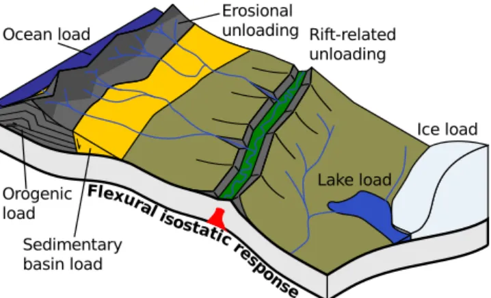
Flexure of the lithosphere is a frequently observed processes by which loads bend the elastic outer shell of Earth or other planets (Watts, 2001; Watters and McGovern, 2006). The sources of these loads are wide-ranging (Fig. 1), encompass-ing volcanic islands and seamounts (Watts, 1978; Watts and Zhong, 2000), mountain-belt-forming thrust sheets and their associated subsurface loads (Karner and Watts, 1983; Stew-art and Watts, 1997), sedimentary basins (Watts et al., 1982; Heller et al., 1988; Dalca et al., 2013), continental ice sheets (Le Meur and Huybrechts, 1996; Gomez et al., 2013), lakes (Passey, 1981; May et al., 1991), seas and oceans (Gov-ers et al., 2009; Luttrell and Sandwell, 2010), extensional tectonics (negative loads) (Wernicke and Axen, 1988), ero-sion (negative loads) (McMillan et al., 2002), mantle plumes (basal buoyant and therefore negative loads) (D’Acremont et al., 2003), and more.
Theory to describe deflections of the lithosphere under loads has evolved significantly over the past 160 years (Watts, 2001). The development of this theory started with simple approximations of perfect buoyant compensation of loads by a lithosphere with no strength overlying a mantle of known density (Airy, 1855; Pratt, 1855). These approxima-tions allowed surveyors to explain the observed lack of sig-nificant gravity anomalies around large mountain belts (cf., Göttl et al., 2009). While this theory, called isostasy, revolu-tionized the way topography was viewed on the Earth, more realistic solutions for isostatic deflections of the surface of Earth take into account the bending, or flexure, of a litho-spheric plate of nonzero but finite strength. This strength may be defined as theelastic thickness, the effective thickness of
Figure 1.Flexural isostasy can be produced in response to a range
of geological loads.
rigiditythat is characteristic of a plate of a given thickness (see Eq. A7). By bending over distances of several tens to hundreds of kilometers, the lithosphere low pass filters a dis-continuous surface loading field into a smoothed solid-Earth response.
Even though the early geological theories of Pratt (1855) and Airy (1855) focused on simple buoyancy, the differential equation basis for solving lithospheric bending already ex-isted at that time. Bernoulli (1789) and Germain (1826, and earlier work) developed the first differential-equation-based theories for plate bending. Lagrange (1828) reviewed the prize that Germain won in 1811 for her work on elastic plate flexure, and, on realizing an error in the lumping of terms due to Germain’s incorporation of an incorrect formula by Eu-ler (1764), corrected it and produced the first complete flex-ure equation (see reviews by Todhunter and Pearson, 1886; Ventsel et al., 2002). Around the same time, Cauchy (1828) and Poisson (1828) better connected the theory of elasticity to plate bending problems. These works predated Kirchhoff (1850), who developed theclassicalorKirchhoff–Loveplate theory that remains in use today (Ventsel et al., 2002). While many further advances have been made (e.g., Love, 1888; Timoshenko et al., 1959) especially for structural and aero-nautical engineering, it is the Kirchhoff–Love plate theory that has been used most widely for geological applications (e.g., van Wees et al., 1994). Comer (1983) tested classical Kirchhoff plate theory, which is athin-platetheory that sim-plifies the plate geometry and therefore the mathematics re-quired to solve for it, against a thick-platetheory of litho-spheric flexure. While this thick-plate theory relaxes several approximations, its solutions are very similar to those for thin-plate flexure (Comer, 1983).
In the first half of the twentieth century, Vening Meinesz (1931, 1941, 1950) and Gunn (1943) applied analytical so-lutions of the plate theory of Kirchhoff (1850) to geological problems. They employed analytical solutions that relate the curvature of the bending moment of a plate of uniform elastic properties to an imposed surface point load, line load, or
si-nusoidal load. These load solutions could be used to compute flexural response to any arbitrary sum of individual loads in either the spatial or spectral domain, due to the linear nature of the biharmonic flexure equation (Eqs. 1 and 2), and may be combined with a variety of boundary conditions (Watts, 2001).
Computational advances allowed discretized models to re-place purely analytical solutions. These models fall into one of several categories. Many take advantage of the linear na-ture of the flexure equation for constant elastic thickness to superimpose analytical solutions of point loads (in the spa-tial domain) or sinusoidal loads (in the wavenumber domain) in order to produce the flexural response to an arbitrary load (Comer, 1983; Royden and Karner, 1984). Other models pro-duce numerical solutions to the thin plate flexure equation by solving the local derivatives in plate displacement with numerical (mostly finite difference) methods (e.g., Bodine et al., 1981; van Wees et al., 1994; Stewart and Watts, 1997; Pelletier, 2004; Govers et al., 2009; Sacek et al., 2009; Wick-ert, 2012; Braun et al., 2013). Models in this latter category allow for variations in the elastic thickness of the plate, a fac-tor of growing importance as variations in elastic thickness through space and time are increasingly recognized, mea-sured, and computed (e.g., Watts and Zhong, 2000; Watts, 2001; Van der Lee, 2002; Flück, 2003; Pérez-Gussinyé and Watts, 2005; Tassara et al., 2007; Pérez-Gussinyé et al., 2007, 2009; Tesauro et al., 2009; Kirby and Swain, 2009, 2011; Lowry and Pérez-Gussinyé, 2011; Tesauro et al., 2012b, a, 2013; Braun et al., 2013; Kirby, 2014). In spite of these ef-forts, the community currently lacks a robust, easy-to-use, generalized tool for flexural isostatic solutions that can be used by modelers and data-driven scientists alike.
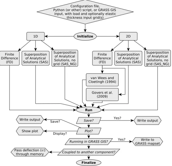
Here I introduce a broadly implementable open-source package of solutions to flexural isostasy. This package, called gFlex (for GNU flexure), advances and makes more ac-cessible an earlier model, generically calledflexure (Wick-ert, 2012). gFlex has been released under the GNU Gen-eral Public License (GPL) version 3 and is made avail-able to the public at the University of Minnesota Earth-surface GitHub organizational repository, at https://github. com/umn-earth-surface/gFlex, and through the Python Pack-age Index (PyPI). This allows for rapid collaborative editing of the source code and easy automated installation. It is writ-ten in Python (e.g., Rossum et al., 2012) for easy interoper-ability with a range of other programming languages, mod-els, and geographic information systems (GIS) packages, and to take advantage of the numerical packages for Python that allow for much more rapid matrix solutions than would be typical with a more basic interpreted language (Jones et al., 2001; Davis, 2004; Oliphant, 2007; van der Walt et al., 2011). See Section 5 for further information on obtaining and run-ning gFlex.
Figure 2.Flowchart for gFlex as either a standalone model with configuration and input files, a Python module or coupled component in a
modeling framework, or a GRASS GIS component.
the spatial domain (i.e., as a sum of Green’s functions) (e.g., Royden and Karner, 1984). These use biharmonic equation for plate flexure with uniform elastic properties (Eqs. 1 and 2) (Bodine et al., 1981). Second, it can compute finite dif-ference solutions for both constant and arbitrarily varying lithospheric elastic thickness structures. These solutions fol-low the work of van Wees et al. (1994), and hence Braun et al. (2013), except that gFlex does not incorporate terms for end loads but does include a wider range of implementable boundary conditions (Table 1). gFlex can be run as a stan-dalone program with an input file, as a component of the in-development Landlab landscape modeling framework (Hob-ley et al., 2013; Tucker et al., 2013, 2015) and by extension as a component within the Community Surface Dynamics Mod-eling System (CSDMS) (Syvitski et al., 2011; Overeem et al., 2013), or as a pair ofadd-onsto the Geographical Resources
Analysis Support System (GRASS) Geographic Information System (GIS) (Neteler et al., 2012). The GRASS GIS imple-mentation is particularly important, as it provides pre-built and standardized command-line and graphical interfaces and
the ability to directly pull inputs from and compare solutions against field data in their native coordinate systems.
2 Methods and model development
Table 1.Boundary conditions. Names provided here are the same as those used in the model, and b.c. stands for boundary condition. The first five can be selected for numerical solutions. The final one, NoOutsideLoads, is the outcome of superposition of analytical solutions, which allows the entire space to respond to local loads as if the 0-deflection boundaries were infinitely far away. In this notation, the subscript b indicates the boundary, generically. Where 0 andnare included as subscripts, i.e., for the mirror and periodic boundary conditions, these indicate boundaries at the first and last node of the model domain along a particular axis. Subscriptx, which is a stand-in forxory, is a
variable distance to indicate the symmetry across a mirror boundary. Each of these boundary conditions requires a corresponding boundary condition for flexural rigidity.
Name Mathematical Description Rigidity b.c.
0Displacement0Slope wb=0 no displacement at boundaries d
2D b
dx2 =0 0Moment0Shear d2wb
dx2 =d 3w
b
dx3 =0 broken plate with a free cantilever end d 2D
b
dx2 =0 0Slope0Shear dwb
dx =d
3w b
dx3 =0 free displacement of a horizontally clamped boundary d 2D
b
dx2 =0
Mirror wb=n−x=wb=n+x plane of mirror symmetry at boundary Db=n−x=Db=n+x
Periodic wb=n=wb=0 wrap-around boundary: infinite tiling of model domain Db=n=Db=0
NoOutsideLoads w∞=0 produced by analytical solutions with uniformD dDdxb =0
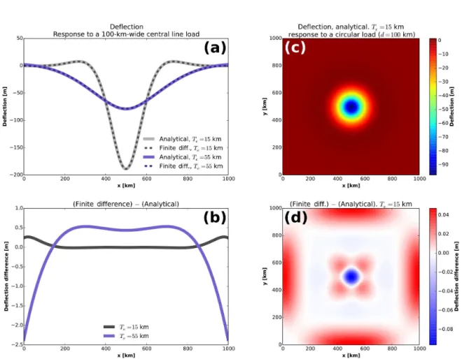
Figure 3.Numerical (FD) and analytical (SAS) solutions in one dimension(a)and two dimensions(c)and their differences(b, d)in response to a 100 km (long/in diameter) central line/circular load. These differences are due primarily to the NoOutsideLoads boundary condition of the analytical solution and the 0Displacement0Slope boundary condition of the numerical solution. This can be seen in panel(b)where the
example with a lower elastic thickness is less offset due to the greater number of flexural wavelengths between the load and the boundary, and in the greater agreement between the solutions on the longer diagonal boundaries in(d). The offset in the middle, visible as a small bump
2.1 Superposition of analytical solutions
The first solution type takes advantage of the linear nature of the analytical solution for flexure of a plate of constant thickness and elastic properties when subjected to a point or line load. These solutions may be superposed (i.e., summed) in space to compute the full flexural response. The sec-ond approach is to solve the equation for lithospheric flex-ure as a matrix equation by employing a finite difference scheme. This employs a sparse matrix elimination solver (e.g., Davis, 2004). The primary gFlex finite difference solu-tion follows the approach of van Wees et al. (1994) to permit computations with steep gradients in flexural rigidity (Ap-pendix Sect. A2), but gFlex also offers the discretization of Govers et al. (2009).
The analytical solution imposes the assumption that scalar flexural rigidity,D, is uniform. This leads to biharmonic ex-pressions for plate bending in one and two dimensions, re-spectively:
Dd
4w
dx4 +1ρgw=q, (1)
D∇4w=D∂ 4w
∂x4 +D ∂4w
∂y4 +2−D ∂4w
∂x2∂y2+1ρgw=q. (2)
Here, w is vertical deflection of the plate,q is the applied
surface load, and1ρ=ρm−ρf is the density of the mantle minus the density of the infilling material; see Fig. A1 for a diagrammatic description of all variables. The1ρterm
rep-resents the feedback by which flexural subsidence can lead a depression to be filled by material, which leads to addi-tional flexural subsidence. This can occur, for example, in a system that is fully underwater (e.g., an underwater volcano load) or one in which the depression is completely filled with sediments. If this infilling material is not uniform in density and/or spatial extent – for example, due to onlap or offlap of water along a shoreline – then one may solve this feedback instead via iteration, by solving forρf =ρair≈0 and adding water (or another load) to regions that match certain condi-tions after every cycle of the iteration.
The above equations are linearizable, and therefore can be solved by superposition of analytical solutions. In gFlex, this is done in the spatial domain on both structured grids and as a response to an arbitrarily placed set of point loads. Spectral solutions are possible (Stephenson, 1984; Stephenson and Lambeck, 1985) and efficient using fast Fourier transform al-gorithms (cf. Welch, 1967), but have not been implemented. The one- and two-dimensional solutions for lithospheric flex-ure take the form of an exponentially damped sinusoid. In one dimension, this is represented by the following expres-sion:
wi =q
α31-D
8D e
(x−xi) α1-D
cos
x −xi
α1-D
+sin x
−xi
α1-D
. (3)
Here, the i subscript indicates that this is the response to
a line load at a single x position, xi. α1-D is the
one-dimensional flexural parameter, defined by Vening Meinesz (1931) (following Hertz, 1884):
α1-D= 4D
(1ρ)g
1/4
. (4)
The significance of the flexural parameter is that the flex-ural wavelength,λα is related to the flexural parameter as
λα=2π α. The distance from a point load to the first flexural bulge (forebulge) that it creates around its local depression, for example, is a flexural half-wavelength,π α. This nature of plate bending as an exponentially decaying periodic func-tion can be seen most easily in the one-dimensional analyti-cal (constantTe) solution in Eq. (3).
Brotchie and Silvester (1969) derived that the exponen-tially damped sinusoid due to a point load in two dimen-sions should be expressed by kei (Abramowitz and Stegun, 1972), which is the zeroth-order Kelvin function that satis-fies the equation ker(r)+ikei(r)=K0 reπ i/4, whereK0is the zeroth-order modified Bessel function of the second kind. This function was defined by Lord Kelvin to solve for elec-trical current density in a circular wire with an applied os-cillating (alternating) current (Barron and Barron, 2012, Ap-pendix 5), and its solution has been broadly applied to the two-dimensional bending of a plate (e.g., Timoshenko et al., 1959; Lambeck, 1981; McNutt and Menard, 1982; Watts, 2001).
wi,j=q
α22-D
2π Dkei
q
(x−xi)2+(y−yj)2
α2-D
(5)
α2-D= D
(1ρ)g
1/4
(6) The subscriptsi, j indicate that this is the flexural response
to a single point load at thex andypositionsxiandyj. The two-dimensional flexural parameter,α2-D, containsDinstead
of 4D in the numerator because it does not need to include implicit loads and deflections along theyorientation that are required in the one-dimensional line-load plate bending case. Lithospheric flexure calculated by superposition of analyt-ical solutions can be represented as a simple sum across all line loadsqlor point loadsqp:
w=X
ql
wi (1−D), (7)
w=X
qp
wi,j (2−D). (8)
linear dimensions of the solution array, and is subsampled and re-scaled to compute the distributed response to each cell in the grid that contains a load. This technique works for all for rectilinear grids with uniformx andy grid spac-ing, though thexandygrid spacing do not have to be equal to one another. A similar optimization is possible for one-dimensional solutions, but these are so rapid that this has not been found to be necessary. Within gFlex, this solution type is termed SAS, which stands for superposition of analytical solutions.
The analytical solution response to point or line loads can also be computed for a scattered set of loads and a scattered (and not necessarily the same) set of points at which the flexural response is calculated. This solution type is termed SAS_NG, which stands for, superposition of analytical so-lutions: no grid. Because it lacks the grid uniformity that permits the a solution template to be used, its computational time is not optimized in this way (Sect. 2.5).
2.2 Finite difference solutions
Finite difference solutions in one and two dimensions em-ploy Eqs. (A19) and (A20), respectively. For these solutions, dxand dymay differ from one another, but each must be con-stant. First, for the one-dimensional solution, the expansion of Eq. (A19) is
D∂
4w
∂x4 +2 ∂D
∂x ∂3w ∂x3 +
∂2D ∂x2
∂2w
∂x2 +1ρgw=q. (9)
The two-dimensional solution is based on an expansion of Eq. (A20) (van Wees et al., 1994):
D∂
4w
∂x4 +D ∂4w
∂y4 +2−D ∂4w ∂x2∂y2
+2∂D
∂x ∂3w ∂x3 +
∂2D ∂x2
∂2w ∂x2 +2
∂D ∂y
∂3w ∂y3 +
∂2D ∂y2
∂2w ∂y2
+ν∂ 2D
∂y2 ∂2w
∂x2 +ν ∂2D
∂x2 ∂2w
∂y2 +2 ∂D
∂x ∂3w ∂x∂y2+2
∂D ∂y
∂3w ∂x2∂y
+2(1−ν)∂
2D
∂x∂y ∂2w
∂x∂y +1ρgw=q. (10)
These equations are discretized using a second-order ac-curate centered finite difference approximation (Fornberg, 1988, Table 1).
Finite difference solutions in two dimensions may also be generated following the solution and discretization of Govers et al. (2009), which produces solutions for a more limited range of flexural rigidity variations.
The finite difference solution is computed as a linear ma-trix equation,
AW =Q, (11)
where Ais a sparse matrix of operators from a linear de-composition of Eqs. (A19) or (A20), W is a vector of de-flections (typically unknown), andQis a vector of imposed
loads (typically known). It is solved directly by using the sparse LU (lower upper) factorization package UMFPACK (unsymmetric-pattern multifrontal package) (Davis, 2004) or, at the user’s choice, iteratively with one of the many solvers that are available with the SciPy (Scientific Python) package (Jones et al., 2001).
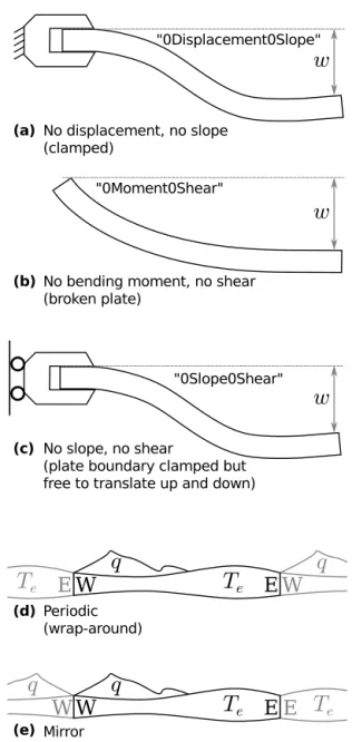
2.3 Boundary conditions
gFlex supports a number of boundary conditions, and these are summarized in Table 1 and schematically drawn in Fig. 4. The finite difference (sparse matrix) nu-merical solutions can freely define any combination of displacement-and-slope (0Displacement0Slope), no-bending-moment-and-no-shear (0Moment0Shear), no-slope-and-no-shear (0Slope0Shear), and mirror boundaries. Peri-odic boundaries may be mixed with any combination of the aforementioned boundary conditions, with the requirement that they exist on both sides of the deflection array, as having (for example) deflections at the west end of the array sensi-tive to loading and deflections to the east, but with those on the east not, in turn, sensitive to the west, being nonsensical. Superposition of analytical solutions naturally produce a 0-displacement boundary at infinite distance from each point load (NoOutsideLoads). This can be seen by solving Eqs. (3) and (5) asx→ ∞andy→ ∞. Each of these boundary
con-ditions can be related to geological processes or locations that one may wish to model (Fig. 5).
The 0Displacement0Slope (orclamped) boundary condi-tion (Fig. 4a) may be used to approximate a NoOutsideLoads case for the finite difference solutions (Fig. 3). When placed one flexural wavelength away from a point or line load, the surface displacement should, for a plate of constant elastic thickness, be∼0.2 % of that at the point of maximum deflec-tion, which is negligible compared to most sources of geolog-ical error. It is conceivable that a difference in elastic thick-ness in a continuous plate may exist that is so great that the thicker plate can be approximated to not bend; a 0Displace-ment0Slope boundary condition may also be used to simulate this, though one must debate whether to do this or to compute the flexural response across a plate with a prescribed elastic thickness variability.
Figure 4.Schematics of boundary condition types allowed in the
finite difference solutions to gFlex.
suited for continental rift zones (Burov et al., 1994), as these closely approximate a linear discontinuity in an otherwise thick lithosphere. In all three of these cases, the lithosphere should lose strength as it approaches the boundary condition. For this reason, 0Moment0Shear is implemented only for the finite difference solution, which allows for spatial variations in elastic thickness.
The 0Slope0Shear boundary condition (Fig. 4c) may be considered to be a flat clamp on the boundary of the plate that may be freely moved upwards or downwards. While it may require creative thought to uncover a geological pro-cess that holds a plate edge flat but allows it to move freely in the vertical, this boundary condition can also be used at an appropriate distance away from the load(s) to approxi-mate a NoOutsideLoads boundary for a finite difference
so-lution, though typically the 0Displacement0Slope boundary provides a closer match.
Theperiodicboundary condition (Fig. 4d) wraps one side of the model around to the other side such that they form an infinite loop. To visualize this, one may imagine taking a pa-per map and taping either the east and west sides together or the north and south sides together, such that the flexure in-duced by loads on one edge is continuous with load-inin-duced flexure on the opposite edge. Elastic thickness and loads both wrap around this boundary, making it possible to, if one is not careful, create sudden jumps in elastic thickness at the edge of the model. This takes somewhat longer to solve (Fig. 6c), but can be useful to compute a flexural response to the load of a long mountain belt by modeling just a limited region perpendicular to the strike of the range crest and allowing this slice to infinitely repeat in the range-crest-parallel ori-entation; at the limit of a very narrow slice of model space, this approaches the one-dimensional line-load solution. If a future model of lithospheric flexure relaxes the current as-sumption in gFlex that dx and dy may be different but must be constant in space, the periodic boundary condition should enable a finite difference flexural model to be employed on a closed surface, such as a sphere, enabling full global model-ing. This is, to the best knowledge of the author, the first time that a periodic boundary condition has been implemented for lithospheric flexure.
Themirrorboundary condition (Fig. 4e) reflects the
elas-tic thickness and load structure across a plane of symme-try at the boundary. This may be used to speed a solution where a plane of mirror symmetry may be implied, which is important for large grids or where gFlex is used as part of a coupled set of numerical models (e.g., through CSDMS: Syvitski et al., 2011; Overeem et al., 2013; Peckham et al., 2013; Tucker et al., 2015). Example usage cases include to-pographic unloading by erosion of a symmetrical mountain range (Fig. 5c, and 5d), isostatic adjustment under a sym-metrical ice cap, and emplacement of a volcanic load. The latter two cases often have fully radial symmetry, and there-fore may be placed at the corner of the solution array with mirror boundary conditions on both adjacent sides to fur-ther limit the needed computational area. This is also to the best knowledge of the author the first application of a mir-ror boundary condition to modeling of lithospheric flexure, which is surprising considering its potential utility.
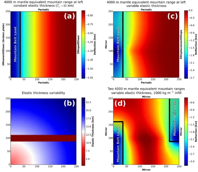
Figure 5.Example runs of gFlex with varying elastic thickness and boundary conditions.(a)depicts a long north–south mountain belt and foreland basin under uniform elastic thickness.(b)provides a contrived field of variable elastic thickness.(c)is similar to(a)except in that it uses a mirror boundary for a symmetrical mountain belt over a continuous lithospheric plate instead of a broken-plate solution, and that the plate has the variable elastic thickness structure given in(b).(d)depicts the flexural interaction of two mountain belts on the same variable-elastic-thickness lithosphere shown in(b)and has mirror boundary conditions at all edges.
as well. For the analytical solutions, the approximation is an infinite plate of constant elastic thickness.
In two-dimensional solutions, boundary conditions meet at corners. Where a boundary condition meets another of the same boundary conditions at the corner, the two generate a continuous boundary condition that includes the corner of the array. This is always the case for the analytical solutions with implicit NoOutsideLoads boundary conditions. Where mirror or periodic boundary conditions meet themselves at corners, these produce doubly reflecting or doubly periodic boundaries; if every boundary is mirror or periodic (neces-sary in the latter case as periodic boundary conditions must always exist as pairs on opposite sides), these generate an in-finite tessellated plane of loads and elastic thicknesses. Some boundary conditions in gFlex can work harmoniously with others. Periodic and mirror boundary conditions propagate
0Moment0Shear, 0Slope0Shear, and 0Displacement0Slope boundary conditions that exist orthogonally to them. Where mirror and periodic boundary conditions intersect at a corner, the periodic boundary condition will propagate the mirror boundary to±∞. Those boundary conditions that do not re-flect or repeat the effects of the other boundary conditions do not share the corners equally: in gFlex, 0Displacement0Slope boundary conditions dictate all corners where they meet other boundary conditions, forcing them to remain fixed at 0; physically, this means that theclamp of the
Figure 6.Model benchmarking.(a)The ungridded superposition of analytical solutions (SAS_NG) computation time is proportional to
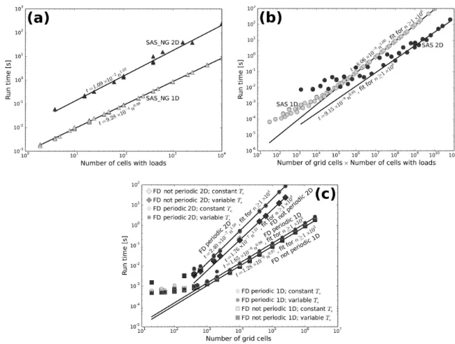
the number of cells with loads present, as the solutions are calculated once for each of these positions.(b)The gridded superposition of analytical solutions (SAS) scales with the total number of grid cells times the number of cells with loads, as this is the total number of computations that must be made.(c)Finite difference solutions are computed with sparse matrices with dimensions equal proportional to the grid dimensions, squared, and therefore scale with the number of total grid cells. All of the solution time relationships are close to linear except for the two-dimensional finite difference solutions, due to the added complexity of their finite difference stencil. Many fits are to a subset of the data to avoid those solutions that are so rapid that the amount of time required for the non-solver portions of the code becomes significant. All marker symbols are semi-transparent, meaning that darker symbols than those that appear in the legend imply additional data points underneath.
and Watts, 1997), while the 0Slope0Shear boundary condi-tion has not.
2.4 Discontinuities and limit asTe→0
Two notable issues inherent to the finite difference solutions and the treatment of a continuous plate become apparent as
Te→0. The first is that a region ofTe=0 must have a width of at least three cells to produce the expected local isostatic equilibrium; this is a result of numerical diffusion in the cen-tral difference discretization provided in Eqs. (9) and (10). The second is that because any region of 0 elastic thickness will enter isostatic equilibrium with its local loads and not be affected by nonlocal effects; if this region lies along the edge, it will ignore all boundary conditions. If a Te=0 re-gion along a boundary is≥3 cells wide, it imposes a 0Dis-placement0Slope boundary condition on the interior cells;
smaller regions ofTe=0 will allow some information on the ultimate boundary condition to leak through via numerical diffusion.
loads, which are not currently included in gFlex, could be used in combination with a 0Moment0Shear boundary con-dition to better parameterize faults (e.g., van Wees et al., 1994) and expand the utility of gFlex. However, the typical case for which gFlex is designed involves glacial-isostatic adjustment, large-scale water loads, sedimentary basin devel-opment, large-scale erosional unloading, and other processes that extend across a swath of heterogeneous lithosphere that may contain many faults. In these cases, it has been found to be sufficient to simply characterize a variable field of finite elastic thickness across the domain, where elastic thickness falls around fault zones (e.g., Manríquez et al., 2013). 2.5 Model benchmarking
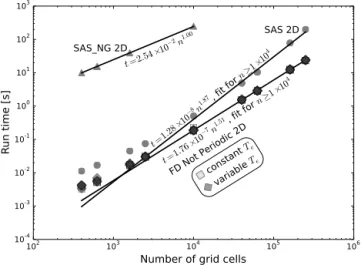
A set of tests was performed to measure the speed at which gFlex computes solutions. In these tests, an elastic plate that is 1000 km long (one-dimensional and two-dimensional) and 1000 km wide (two-dimensional) is subjected to a square load at its center that ranges from 100 km to the full 1000 km on each side. This load places a normal stress of 9 702 000 Pa on the surface, which is equal to 300 m of mantle material (3300 kg m−3). In these scenarios, there is no assumed infill-ing material (ρf =0). gFlex computed solutions for uniform rectilinear grids of increasing size using gridded and ungrid-ded superposition of analytical solutions (SAS and SAS_NG, respectively) and finite difference (FD) methods. All bound-ary conditions (Table 1 and Fig. 4) were tested, though not in combination. The finite difference solutions include scenar-ios with both constant (25 km) and variable (10–40 km) ef-fective elastic thickness, with the latter varying sinusoidally over a wavelength of 500 km such that the plate contains two fullTecycles. In the two-dimensional case,Tevaries in both dimensions to produce a smoothed checkerboard pattern of elastic thickness. Finite difference solutions reported employ the direct solver UMFPACK (Davis, 2004), as it has been bet-ter tested in gFlex than the ibet-terative solution methods and is therefore the default solver. Fig. 6 displays computation time for all of the benchmarking tests, and Fig. 7 is a comparison of the SAS_NG, SAS, and FD solution techniques for the case in which every point at which the solution is calculated also contains a nonzero load. These solution times do not ac-count for file input or output or graphics generation. They do include the initialization time for the solution steps of gFlex; therefore, a number of the power-law fits to solution time do not include the times calculated with the smallest arrays, for which initialization time is a significant fraction of the total model runtime.
The factors that determine computation time are the so-lution method and the inclusion of periodic boundary con-ditions. While the SAS_NG method scales the best with in-creasing grid size, it is so much slower than the other meth-ods for standard model-run grid sizes that it will not often ex-ceed their speed. The finite difference method is the fastest if every cell contains a load, but can become slower than the
an-Number of grid cells
Figure 7.Comparison between solution methods where every cell in the domain contains a load. The ungridded superposition of an-alytical solutions (SAS_NG) scales best but in these tests is the slowest. It can, however, be faster when fewer cells contain loads. Some fits are to a subset of the data to avoid those solutions that are so rapid that the amount of time required for the non-solver por-tions of the code becomes significant. All marker symbols are semi-transparent, meaning that darker symbols than those that appear in the legend imply additional data points underneath.
alytical methods if only a few cells contain loads, as analyti-cal methods must make one set of analyti-calculations across the grid per load. Standard runtimes are between a fraction of a sec-ond and a few minutes on a personal laptop computer (Dell XPS 13 Developer Edition running Ubuntu 14.10) (Figs. 6 and 7).
3 Model interfaces and coupling
Some users of gFlex may want to run a single calculation, while others may want to produce many solutions as part of a larger-scale numerical modeling exercise, such as an in-version for elastic thickness or coupling with another model. Therefore, four different methods to use gFlex have been pre-pared:
1. standalone, with input files; 2. as part of a Python script;
3. driven by GRASS GIS (Neteler et al., 2012) to simplify integration of geospatially registered data with the litho-spheric flexure model;
GRASS GIS integration is also possible for model coupling using Python, including efforts that use the Landlab frame-work.
3.1 Standalone with input files
Some users may want to employ gFlex as a single calcula-tion, for example to calculate the flexural response to a set of loads generated by a sedimentary deposit that was mea-sured in the field. The user prepares an input file of model settings, an input ASCII grid of loads, and, should the elastic thickness be nonuniform, an input ASCII grid of lithospheric elastic thicknesses. Outputs from this mode of running gFlex include an ASCII grid of surface deflections and a set of plots of surface deflections and loads.
3.2 As part of a Python script
gFlex may also be imported as a Python module to be run either as a standalone simulation or as a component in a multi-model integration effort. This allows it, for example, to be a part of a flexural backstripping toolchain or a model of glacial-isostatic adjustment. Backstripping calculations may be performed by simply removing the sedimentary load (Roberts, 1998), or, in the case of a foreland basin, by in-verting for the mountain belt loading history and lithospheric elastic thickness that would be required to produce the basin (Ballato et al., 2016). A programmatic approach is also use-ful for scenarios in which material infills a depression, but not over the whole domain and/or not with uniform density. While the flexure equations require that ρf be constant, a more flexible way to solve for the effect of infilling mate-rial is to compute flexural response withρf =ρair≈0, add loads based on some set of rules, and then re-calculate flex-ure iteratively until convergence is achieved. This can occur in regions with a complex set of sedimentary deposits (see also Watts et al., 1982; Watts, 2001) and/or to be used for seawater loading across a shoreline (see also Mitrovica and Milne, 2003).
3.3 Driven by GRASS GIS
gFlex is also prepared for integration with the open-source geospatial software GRASS GIS (Neteler et al., 2012) as two add-ons or extensions named r.flexure and v.flexure, which are raster and vector operations, respectively. As GRASS GIS is a map-based application, r.flexure and v.flexure employ two-dimensional solutions (both analytical and fi-nite difference), though future extensions of these mod-ules to compute flexure from line loads along chosen one-dimensional profiles would be possible. r.flexure can use the finite difference or SAS solution methods, whereas v.flexure exclusively uses the SAS_NG solution method to take advan-tage of its ability to produce solutions for an arbitrary scatter of point loads. Advantages of GRASS GIS include
1. full integration within a geospatially registered environ-ment, meaning that data can be used directly as model inputs, and that model outputs may be compared against data;
2. a documented and standardized command-line inter-face;
3. a pre-built and standardized graphical user interface (GUI).
The graphical user interface is incorporated into the GRASS GIS wxPython GUI (Landa, 2008; Neteler et al., 2012), and this is particularly helpful for researchers, who are not as ac-customed to command-line interaction with computers to use gFlex with their data. For computer modelers, the GRASS GIS coupling may be used to support broader model cou-pling and data–model integration efforts (see, for example, Srinivasan and Arnold, 1994).
3.4 Modeling frameworks
CSDMS (broadly) and Landlab (in particular) both include methods for integrating modular blocks of code as part of their respective efforts towards the community-wide goal to make modeling of Earth systems less time intensive and more streamlined (Voinov et al., 2010; Syvitski et al., 2011; Overeem et al., 2013; Peckham et al., 2013; Hobley et al., 2013; Tucker et al., 2013, 2015). gFlex is included as a mod-ular component of the still-in-development Landlab Earth-surface modeling framework (Hobley et al., 2013; Tucker et al., 2013, 2015). Landlab integration provides wrapping with the CSDMS Basic Model Interface (BMI) and Com-ponent Model Interface (CMI) using the CSDMS Stan-dard Name construction conventions (Peckham et al., 2013). The standard interfaces provided by both of these model-ing frameworks will streamline model couplmodel-ing that uses gFlex and help to prevent duplication of effort in building plate bending models. Furthermore, the inclusion of gFlex in Landlab will allow numerous Earth-surface systems to be modeled more precisely (Fig. 1).
4 Application example: Iceland
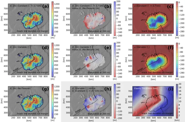
Figure 8.This coupled model run for a hypothetical extent of the Iceland ice cap shows the influence of a variable elastic thickness structure
(i). The areal extent of the three ice caps is nearly identical(a, d, g)in this small-scale and largely topographically controlled example.
Flexural isostasy with a constant 3.7 km elastic thickness(c)(following Hubbard, 2006) reduces ice cap extent and causes some interior ice thickening when compared to the case without flexure(b), as the ice cap conforms to the bowl-shaped depression that it creates. Deformation
in the case with variable elastic thickness(f)is focused along the ridge and extends farther on the southwestern side that has greater elastic thickness, and modifies the topography of western Iceland (low elastic thickness) to produce spatially variable ice thickness changes(e, h).
the unique intersection of the Iceland hotspot and the Mid-Atlantic Ridge, which together produce a weak lithosphere with spatially variable elastic thickness, resulting in short-wavelength variability in the solid-Earth response to loading. Here I test the two-way coupling between ice dynamics and solid-Earth deformation and the differences in steady-state ice caps that are produced in a modest climate change and ice cap extent scenario.
This coupled ice dynamics and flexural isostatic model of Iceland requires four input components: the elastic thick-ness structure around Iceland, the modern topography of Ice-land, the modern surface temperature field of IceIce-land, and modern precipitation rates across Iceland. The ice cap model used here (cf. Colgan et al., 2015) employs a shallow-ice ap-proximation with basal sliding as a linear function of driving stress, which is intentionally much simpler than the modeling approach (Hubbard, 2006) that Hubbard et al. (2006) used to model the Last Glacial Maximum (LGM) Iceland Ice Cap. This is because the goal here is to show schematically the
importance of including lateral variations in elastic thickness on the reconstructed thickness of an ice cap for a given pa-leoclimate, with less emphasis on actually reproducing any particular extent of the Iceland Ice Cap.
The elastic thickness structure under Iceland, in this schematic example, is related to the age of the oceanic crust. Calmant et al. (1990) related elastic thickness to the age of the lithosphere with the simple equation that results from the square-root time dependence of lithospheric cooling via ther-mal conduction (cf. Stein and Stein, 1992):
Te=(2.70±0.15) √
1t . (12)
Here,Teis given in kilometers and the age of the lithosphere,
(Neteler et al., 2012). The regional age of oceanic crust is provided by Müller et al. (2008), but their map indicates that even crust at the ridge in Iceland has an age of 6–7 Ma, re-sulting in a greater computed effective elastic thickness than would be expected based on the presence of the ridge or from heat flow data (e.g., Flóvenz and Saemundsson, 1993). While the structure of Iceland is certainly more complicated than the simpler parts of the ridge due to the effects of the hotspot and its tectonic environs (e.g., Watts and Zhong, 2000; Foul-ger, 2006), the assumption here is that the lithospheric effec-tive elastic thickness structure due to the ridge is as if young crust continued along the Mid-Atlantic Ridge through all of Iceland, and the elastic thickness map (Fig. 8i) was modified to approximate this for the sake of this example.
The underlying digital elevation model, GEBCO_08 (British Oceanographic Data Centre , BaODC), includes the modern ice caps on Iceland, but these are already flexurally compensated and are small compared to the ice cap modeled here. While their removal would improve reconstructed ice discharge, they are ignored due to the schematic nature of this modeling effort.
Modern temperature and precipitation fields are from the Monthly NOAA-CIRES (National Oceanographic and At-mospheric Administration– Cooperative Institute for Re-search in Environmental Sciences) 20th Century Reanalysis (V2) by Compo et al. (2006, 2011) (for further background on their methods, see Whitaker and Hamill, 2002). These provide twentieth century mean conditions on a 2◦×2◦
latitude–longitude grid (temperature) or a 94×192 Gaussian grid (precipitation). These were cast as point data and inter-polated using splines in GRASS GIS (Neteler et al., 2012). Prior to this spline interpolation, temperature was projected to sea level using the mean cell elevation (with lapse rate of 4.7◦C km−1), following Anderson et al. (2014) for ice caps; after interpolation, the resultant temperatures were then in-terpolated up to their respective surface elevations using the same 4.7◦C km−1 lapse rate. Although not all of the Ice-landic surfaces are covered in ice at present, this rule was prescribed uniformly for the sake of a schematic model.
Three experiments were run: one with no flexure, one with flexure using a constant elastic thickness of 3.7 km (follow-ing Hubbard, 2006, and assum(follow-ing E=65 GPa), and one in
which the full spatially variable flexure was used. In each of these runs, temperature was reduced from its present value by 5◦C and ice expanded to cover an area approximately
equal to the currently subaerially exposed continent, approxi-mately consistent with the previous modeling results of Hub-bard et al. (2006) and with a temperature change that is much less than the LGM drop of 10–13◦C that was predicted to
cause ice to spread onto the continental shelves as well (Hub-bard et al., 2006). Mass balance was simulated by a posi-tive degree-day melt model. June, July, and August temper-atures were used to compute ablation, with a melt factor of 6 mm d−1K−1. Precipitation was held constant and all pre-cipitation was assumed to contribute to positive mass
bal-ance. Each scenario was run for 4000 years to reach full glacial and isostatic equilibrium, with isostatic equilibrium being assumed to occur instantaneously to facilitate more rapid computation of the equilibrium solution.
The results in Fig. 8 summarize the experiments. Figure 8c and f show the modeled flexural isostatic deformation and Fig. 8b and e show the deviation from the case with no isostasy; each of these pairs is for constant and variable elas-tic thickness, respectively. Figure 8h shows that with variable elastic thickness (Fig. 8i), ice thickness variability is concen-trated where lithospheric elastic thickness is low.
The example of isostatic response to ice advance in Iceland is just one possibility of a feedback between an Earth-surface (or other geological) process and flexural deformation. Fur-ther such scenarios involving, for example, orogenesis and foreland basin formation (in settings such as that studied by Ballato and Strecker, 2014), rifting (Braun et al., 2013), and river delta morphologic evolution (Kim et al., 2006), will im-prove our understanding of the dynamic interactions between Earth’s surface and subsurface (e.g., Braun et al., 2013).
5 Code availability
gFlex is available from the University of Minnesota Earth-surface GitHub repository at https://github.com/ umn-earth-surface/gFlex. It runs on Linux, Windows, and Mac computers running Python 2.(X≥7).Y. It may be
downloaded as an archive that is a snapshot of the state of the code, orclonedinto an updatable copy of the software on the computer of an end-user. Version 1.0, described in this pa-per, is stored at https://github.com/umn-earth-surface/gFlex/ releases/tag/v1.0. gFlex is also stored on the Python Pack-age Index (PyPI) at https://pypi.python.org/pypi/gFlex for easy automated download and installed with the command-line tool pip. gFlex documentation is available in its file README.md that is displayed at the main GitHub reposi-tory page, and some additional information is presented at the gFlex CSDMS Wiki page at http://csdms.colorado.edu/ wiki/Model:GFlex.
Interfaces to GRASS GIS and Landlab are available from their respective repositories. The GRASS GIS inter-face works with GRASS GIS 7.X and can be downloaded and installed automatically with the g.extension tool within GRASS (Neteler et al., 2012) or be downloaded through the subversion repository at http://trac.osgeo.org/grass/browser/ grass-addons/grass7. The Landlab interface is located in the Landlab GitHub repository at https://github.com/landlab/ landlab/tree/master/landlab/components/gflex. Both require a locally installed copy of gFlex to run.
6 Conclusions
Appendix A: Derivation: flexure
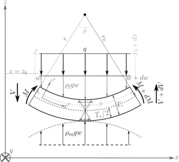
Figure A1.Schematic of the bending of a buoyant plate under a load that is long in theyorientation. This figure highlights the
symme-try in the fiber stresses associated with the bending moment; shear forces should therefore be visualized within each segment of the plate.
Plates resist bending (i.e., flexure) through fiber stresses that develop in response to loading-induced deformation. In this appendix, the background of the theory is provided by an abridged derivation of plate flexure, which provides the back-ground for the assumptions and solution methods employed in both the analytical and finite difference one-dimensional and two-dimensional solutions. Components of the theoret-ical background are also relevant for the various boundary condition options introduced in the main text.
A derivation of flexural response to a load can be subdi-vided into two components. The first is the bending moment, which describes the internally generated torques that resist bending. The second is the relationship between the bending moment and the imposed load.
A1 Bending moments
The bending moment of a plate, M, is the resistance of the
plate to bending. This resistance exists because when a plate of>0 thickness is bent, layers within the plate on the inside of the curve are placed under compression and layers within the plate on the outside of the curve are placed under tension. These fiber stresses are denoted σx′x′ in the along-plate co-ordinate system (x′,z′) depicted in Fig. A1, and cause each infinitesimal layer of the plate to act like a spring that resists plate bending.
Classical (Kirchhoff–Love) plate theory is derived using an approximation of cylindrical bending (cf. Love, 1888).
Over short distances, the bent plate is assumed to follow the arc of a circle (Fig. A1). Arc length,s, is the product of the radius of curvature,rc, and the angle over which the arc is defined,θ.
s=rcθ (A1)
The layer halfway between the top and the bottom of a ho-mogeneous plate experiences no net extension or shortening during bending. This midpoint layer is therefore taken to be the reference radius of curvature,rc=r0, of a plate that ex-tends fromr= −Te/2 tor=Te/2, whereTeis the effective elastic thickness of the plate. Flexural isostatic deflections are small compared to the length scale over which they oc-cur, meaning thatr0≫Te/2, and therefore approximates the true radius of curvature regardless of through-plate position
z′. To calculate the range of arc lengths,s, that exist above and below the reference layer atr0, one can note that Eq. (A1) describes a linear relationship between arc length and radius of curvature. Therefore, it is possible to use the definition of strain and Eq. (A1) to define thefiber strainin each layer as a
function of its distance from the midpoint. The normal strain along thex′orientation,εx′x′, is given by
εx′x′ =
1s
s =
(r0−r)
r0 =
z′
r0. (A2)
Here,z′ is defined to be zero atr0 andθ is held constant and therefore cancels out. Sign conventions are unimportant due to the symmetry of the problem above and below the midpoint layer (Fig. A1).
As radius of curvature decreases, curvature increases:
1
rc ≡
d2z
dx2
1+dxdz
23/2
. (A3)
The long horizontal length-scales involved in flexure prob-lems result in a small slope, (dz/dx)≪1, and this squared becomes so much smaller than 1 that the denominator on the right-hand side≈1. This small slope also allows the small angle approximation to be used, meaning that (x′, y′)≈ (x, y). As noted above, sign convention is unimportant – half
of the plate experiences tension and the other half experi-ences compression – so taking the absolute value, which is included in the definition in order to maintain a positive ra-dius of curvature, becomes unnecessary. Substitutingwforz
andr0forrc, removing the slope-related term in the
numera-tor of Eq. (A3), and combining it with Eq. (A2), provides the magnitude of fiber strains as a function of distance from the midplane in the plate and curvature of the plate:
εxx=εx′x′= z
′
r0=
z′d
2w
Equation (A4) becomes important in the final step to define the bending moment because it relates fiber strains directly to deflections that can be measured and/or modeled.
The bending moment itself,M, balances the torques gen-erated by plate flexure. It therefore describes the resistance of the plate to bending, and is defined as the sum through the thickness of the plate of all fiber stressesσx′x′ times their respective lever armsz′(cf. Turcotte and Schubert, 2002).
M=
Te/2 Z
−Te/2
σxxz′dz′. (A5)
It is possible to rewrite this in terms of strain instead of stress via an elastic constitutive relationship (Hooke’s Law),
σxx=Eεxx+νσyy. Here,E is Young’s modulus, which is a generalized spring constant that typically ranges between 1010 and 1011 Pa for rock (Turcotte and Schubert, 2002, p. 106), and is 65 GPa by default in gFlex. ν is Poisson’s
ra-tio, which describes how much material tends to extend (or shorten) in one direction when shortened (or extended) in another, and is commonly taken to be 0.25 for the
litho-sphere. An analagous equation, σyy=Eεyy+νσxx, exists in they orientation. The stress required for these additional strains reduces the strain in a given orientation by a factor of 1/(1−ν2):
M= E
1−ν2
Te/2 Z
−Te/2
εxxz′dz′. (A6)
In the one-dimensional case,εyy=0. BothEandν lie out-side of the integral because they are assumed constant over
z′.
It is possible to solve for the bending moment in one di-mension by using Eq. (A4) to replaceεxxin Eq. (A6). As the orientation of the curvature (d2w/dx2) is orthogonal to the direction of integration, the integral is simple to solve and results in the solution for the bending moment:
M= ET
3 e 12(1−ν2)
d2w
dx2. (A7)
The terms to the left of the derivative define the scalar flex-ural rigidity,D:
D= ET
3 e
12(1−ν2). (A8)
AsDis the key parameter that controls flexural response, and is a function ofTe,E, and ν, gFlex contains the additional simplifying assumption thatEandνare uniform constants. This permits variations in scalar flexural rigidity to map to variations in effective elastic thickness via Eq. (A8). It pre-vents overparameterization in gFlex, and implicitly states the assumption that changes in the effective elastic thickness of
the lithosphere, cubed, are more significant than changes in Poisson’s ratio, squared, or Young’s modulus.
To generalize the bending moment of a plate that is loaded in two dimensions, one can start by writing a vector of cur-vatures,κ(cf. van Wees et al., 1994):
ˆ κ= ∂2 ∂x2 ∂2 ∂y2 ∂2 ∂x∂y+ ∂2 ∂y∂x ; (A9)
κ= ˆκw=
∂2w ∂x2 ∂2w ∂y2 ∂2w ∂x∂y+
∂2w ∂y∂x = 1 z′ εxx εyy γxy
. (A10)
The first term inκ,εxx/z′, scales with thex-directed nor-mal strain that is also part of the one-dimensional solution.
εyy/z′ is the equivalent for y-oriented fiber normal strains, andγxy/z′is the fiber shear strain term that accounts for tor-sion.
The flexural rigidity must also be defined in three dimen-sions, and is defined here following linear elasticity:
D=D
1 ν 0
ν 1 0
0 0 1−ν 2
. (A11)
Using Eqs. (A10) and (A11), one can define the bending moment as
M=Dκ. (A12)
Solving Eq. (A12) for only the upper (left) terms allows one to recover Eq. (A7), the one-dimensional case.
A2 Force and torque balance
A static lithospheric plate that experiences the downward force of an imposed load, qdx, responds with differential
shear forces,V andV+dV, that develop in response to
bend-ing. Further vertical normal stresses that influence plate flex-ure are generated by the sum of the buoyant restoring force of displaced mantle,ρmg(−w), and additional driving forces by any surface loads that fill the flexural depression,ρfgw. Summed together, these form the additional term−1ρgw, where1ρ=(ρm−ρf)The total vertical force balance is therefore
X
F =qdx−1ρgwdx+(V+dV )−V =0, (A13) dV
dx −1ρgw= −q. (A14)
et al., 1994; Turcotte and Schubert, 2002; Braun et al., 2013). The resultant torque (τ) balance is:
X
τ =M−(M+dM)+dx
2 [−V−(V+dV )]=0. (A15) After noting that dV ≪V, Eq. (A15) simplifies to
dM= −Vdx. (A16)
This can be rearranged to define the shear force as the neg-ative slope of the bending moment, which in turn is propor-tional to the curvature of the deflection (Eq. A7):
V = −dM
dx = −
d dx D
d2w dx2
!
. (A17)
This observation is key to defining the 0Moment0Shear and 0Slope0Shear boundary conditions (Table 1 and Fig. 4).
Equations (A14) and (A17) can be combined by substitut-ingV in Eq. (A14) to relate the bending moment and deflec-tion to the imposed load,q.
d2M
dx2 +1ρgw=q. (A18)
d2 dx2 D
d2w
dx2
!
+1ρgw=q. (A19)
To solve the two-dimensional case, one can follow van Wees et al. (1994) in using the differential operators for cur-vature inκˆ (Eq. A9) to generalize the one-dimensional flex-ural solution. This is then combined with the infill and buoy-ancy term. Written in compact form, the two-dimensional flexural isostatic equation is:
ˆ
Acknowledgements. ADW greatly appreciates Eric Hutton’s insights and help with CSDMS integration and project architecture as well as Daniel Hobley’s work to integrate gFlex with Landlab. Václav Petráš’ help in incorporating gFlex as an official set of GRASS GIS extensions was very much appreciated. Liam Colgan kindly supplied his glacier model source code, and conversations with Robert S. Anderson, Leif S. Anderson, and Gregory E. Tucker helped to inspire the project. The 20th Century Reanalysis V2 data were provided by the NOAA/OAR/ESRL PSD, Boulder, Colorado, USA, from their website at http://www.esrl.noaa.gov/psd/. Funding for this project was provided by the US Department of Defense through the National Defense Science & Engineering Graduate Fellowship Program, the US National Science Foundation Graduate Research Fellowship under grant no. DGE 1144083, an ExxonMo-bil geoscience grant, and by the Emmy Noether Programme of the Deutsche Forschungsgemeinschaft (DFG) through funds awarded to T. Schildgen under grant no. SCHI 1241/1-1.
Edited by: L. Gross
References
Abramowitz, M. and Stegun, I.: Handbook of mathematical func-tions: with formulas, graphs, and mathematical tables, Courier Dover Publications, Mineola, NY, USA, 1972.
Airy, G. B.: On the computation the effect of the attraction of mountain-masses disturbing apparent as the astronomical lati-tude of stations geodetic of surveys, Philos. T. R. Soc. Lond., 145, 101–104, 1855.
Anderson, L. S., Roe, G. H., and Anderson, R. S.: The effects of interannual climate variability on the moraine record, Geology, 42, 55–58, doi:10.1130/G34791.1, 2014.
Ballato, P. and Strecker, M. R.: Assessing tectonic and climatic causal mechanisms in foreland-basin stratal architecture: Insights from the Alborz Mountains, northern Iran, Earth Surf. Proc. Land., 39, 110–125, doi:10.1002/esp.3480, 2014.
Ballato, P., Cifelli, F., Heidarzadeh, G., Ghassemi, M., Wick-ert, A. D., Hassanzadeh, J., Dupont-Nivet, G., Balling, P., Sudo, M., Zeilinger, G., Schmitt, A., Mattei, M., and Strecker, M. R.: Tectono-sedimentary evolution of the northern Iranian Plateau: insights from middle-late Miocene foreland-basin de-posits, Basin Res., doi:10.1111/bre.12180, 2016.
Barron, R. F. and Barron, B. R.: Design for Thermal Stresses, John Wiley & Sons, Inc. Hoboken, NJ, USA, doi:10.1002/9781118093184, 2012.
Bernoulli, J. I. I.: Essai theorique sur les vibrations de plaques elastiques rectangularies et libers, Novi Commentari Acad Petropolit, 5, 197–219, 1789.
Bodine, J. H. H., Steckler, M. S. S., and Watts, A. B. B.: Observa-tions of flexure and the rheology of the oceanic lithosphere, J. Geophys. Res., 86, 3695–3707, doi:10.1029/JB086iB05p03695, 1981.
Braun, J., Deschamps, F., Rouby, D., and Dauteuil, O.: Flex-ure of the lithosphere and the geodynamical evolution of non-cylindrical rifted passive margins: Results from a numerical model incorporating variable elastic thickness, surface pro-cesses and 3D thermal subsidence, Tectonophysics, 604, 72–82, doi:10.1016/j.tecto.2012.09.033, 2013.
British Oceanographic Data Centre (BaODC) and General Bathy-metric Chart of the Oceans (GEBCO): The GEBCO_08 Grid, version 20100927, 2010.
Brotchie, J. F. and Silvester, R.: On crustal flexure, J. Geophys. Res., 74, 5240–5252, doi:10.1029/JB074i022p05240, 1969.
Burov, E. B., Houdry, F., Diament, M., and Deverchere, J.: A broken plate beneath the north Baikal Rift Zone revealed by gravity modelling, Geophys. Res. Lett., 21, 129–132, doi:10.1029/93GL03078, 1994.
Calmant, S., Francheteau, J., and Cazenave, A.: Elastic layer thick-ening with age of the oceanic lithosphere: a tool for prediction of the age of volcanoes or oceanic crust, Geophys. J. Int., 100, 59–67, doi:10.1111/j.1365-246X.1990.tb04567.x, 1990. Cauchy, A.-L.: Sur l’equilibre le mouvement d’une plaque solide,
Exercises de Matematique, 3, 328–355, 1828.
Colgan, W., Sommers, A., Rajaram, H., Abdalati, W., and Frahm, J.: Considering thermal-viscous collapse of the Greenland ice sheet, Earth’s Future, 3, 252–267, doi:10.1002/2015EF000301, 2015. Comer, R. P.: Thick plate flexure, Geophys. J. Int., 72, 101–113,
doi:10.1111/j.1365-246X.1983.tb02807.x, 1983.
Compo, G. P., Whitaker, J. S., and Sardeshmukh, P. D.: Feasibil-ity of a 100-year reanalysis using only surface pressure data, B. Am. Meteorol. Soc., 87, 175–190, doi:10.1175/BAMS-87-2-175, 2006.
Compo, G. P., Whitaker, J. S., Sardeshmukh, P. D., Matsui, N., Al-lan, R. J., Yin, X., Gleason, B. E., Vose, R. S., Rutledge, G., Bessemoulin, P., BroNnimann, S., Brunet, M., Crouthamel, R. I., Grant, A. N., Groisman, P. Y., Jones, P. D., Kruk, M. C., Kruger, A. C., Marshall, G. J., Maugeri, M., Mok, H. Y., Nordli, O., Ross, T. F., Trigo, R. M., Wang, X. L., Woodruff, S. D., and Worley, S. J.: The Twentieth Century Reanalysis Project, Q. J. Roy. Me-teor. Soc., 137, 1–28, doi:10.1002/qj.776, 2011.
Cuffey, K. M. and Paterson, W. S. B.: The physics of glaciers, 4th Edn., Academic Press, Oxford, UK, 2010.
D’Acremont, E., Leroy, S., Burov, E. B., Ã, E. A., Leroy, S., Burov, E. B., D’Acremont, E., Leroy, S., and Burov, E. B.: Numerical modelling of a mantle plume: The plume head-lithosphere in-teraction in the formation of an oceanic large igneous province, Earth Planet. Sc. Lett., 206, 379–396, doi:10.1016/S0012-821X(02)01058-0, 2003.
Dalca, A. V., Ferrier, K. L., Mitrovica, J. X., Perron, J. T., Milne, G. A., and Creveling, J. R.: On postglacial sea level–III. In-corporating sediment redistribution, Geophys. J. Int., 94, 45–60, doi:10.1093/gji/ggt089, 2013.
Davis, T. A.: Algorithm 8xx: UMFPACK V4.3, an unsymmetric-pattern multifrontal method, ACM Transactions on Mathematical Software, V, 1–4, doi:10.1145/992200.992206, 2004.
Euler, L.: Tentamen de sono campanarum, Novi Commentarii Academiae scientiarum Imperialis Petropolitanae, 10, 261–281, 1764.
Flóvenz, O. G. and Saemundsson, K.: Heat flow and geother-mal processes in Iceland, Tectonophysics, 225, 123–138, doi:10.1016/0040-1951(93)90253-G, 1993.
Flück, P.: Effective elastic thickness Te of the
litho-sphere in western Canada, J. Geophys. Res., 108, 2430, doi:10.1029/2002JB002201, 2003.
Foulger, G. R.: Older crust underlies Iceland, Geophys. J. Int., 165, 672–676, doi:10.1111/j.1365-246X.2006.02941.x, 2006. Germain, S.: Remarques sur la nature, les bornes et l’étendue de
la question des surfaces élastiques et équation générale de ces surfaces, imprimerie de Huzard-Courcier, Paris, 1826.
Gomez, N., Pollard, D., and Mitrovica, J. X.: A 3-D cou-pled ice sheet – sea level model applied to Antarctica through the last 40 ky, Earth Planet. Sc. Lett., 384, 88–99, doi:10.1016/j.epsl.2013.09.042, 2013.
Göttl, F., Rummel, R., Geophysics, A., Göttl, F., and Rummel, R.: A geodetic view on isostatic models, Pure Appl. Geophys., 166, 1247–1260, doi:10.1007/s00024-004-0489-x, 2009.
Govers, R., Meijer, P., and Krijgsman, W.: Regional isostatic re-sponse to Messinian Salinity Crisis events, Tectonophysics, 463, 109–129, doi:10.1016/j.tecto.2008.09.026, 2009.
Gunn, R.: A quantitative evaluation of the influence of the litho-sphere on the anomalies of gravity, J. Franklin Inst., 236, 47–66, doi:10.1016/S0016-0032(43)91198-6, 1943.
Heller, P. L., Angevine, C. L., Paola, C., Winslow, N. S., Paola, C., Winslow, N. S., and Paola, C.: Two-phase stratigraphic model of foreland-basin sequences, Geology, 16, 501–504, doi:10.1130/0091-7613(1988)016<0501:TPSMOF>2.3.CO;2, 1988.
Hertz, H.: On the equilibrium of floating elastic plates, Ann. Phys. Chem. 22, 449–455, 1884.
Hobley, D. E. J., Tucker, G. E., Adams, J. M., Gasparini, N. M., Hutton, E. W. H., Istanbulluoglu, E., and Siddhartha Nudurupati, S.: Landlab – a new, open-source, modular, Python-based tool for modeling landscape dynamics, Geological Society of America Abstracts with Programs, 45, p. 649, 2013.
Hubbard, A.: The validation and sensitivity of a model of the Icelandic ice sheet, Quaternary Sci. Rev., 25, 2297–2313, doi:10.1016/j.quascirev.2006.04.005, 2006.
Hubbard, A., Sugden, D., Dugmore, A., Norddahl, H., and Pé-tursson, H. G.: A modelling insight into the Icelandic Last Glacial Maximum ice sheet, Quaternary Sci. Rev., 25, 2283– 2296, doi:10.1016/j.quascirev.2006.04.001, 2006.
Jones, E., Oliphant, T., and Peterson, P.: SciPy: Open source sci-entific tools for Python, http://www.scipy.org/ (last access: 10 February 2015), 2001.
Karner, G. D. and Watts, A. B.: Gravity anomalies and flexure of the lithosphere at mountain ranges, J. Geophys. Res., 88, 10449, doi:10.1029/JB088iB12p10449, 1983.
Kim, W., Paola, C., Voller, V. R., and Swenson, J. B.: Ex-perimental measurement of the relative importance of con-trols on shoreline migration, J. Sediment. Res., 76, 270–283, doi:10.2110/jsr.2006.019, 2006.
Kirby, J. and Swain, C.: Improving the spatial resolution of effective elastic thickness estimation with the fan wavelet transform, Com-put. Geosci., 37, 1345–1354, doi:10.1016/j.cageo.2010.10.008, 2011.
Kirby, J. F.: Estimation of the effective elastic thickness of the lithosphere using inverse spectral methods: The state of the art, Tectonophysics, 631, 87–116, doi:10.1016/j.tecto.2014.04.021, 2014.
Kirby, J. F. and Swain, C. J.: A reassessment of spectral T_e es-timation in continental interiors: The case of North America, J. Geophys. Res., 114, B08401, doi:10.1029/2009JB006356, 2009.
Kirchhoff, G.: Ueber die Schwingungen einer kreisförmi-gen elastischen Scheibe, Ann. Phys., 157, 258–264, doi:10.1002/andp.18501571005, 1850.
Lagrange, J. L.: Note communiquée aux Commissaires pour le prix de la surface élastique décembre 1811, Ann. Chimie Physique, 39, 149–151, 1828.
Lambeck, K.: Flexure of the ocean lithosphere from island uplift, bathymetry and geoid height observations: the Soci-ety Islands, Geophys. J. Int., 67, 91–114, doi:10.1111/j.1365-246X.1981.tb02734.x, 1981.
Landa, M.: New GUI for GRASS GIS based on wxPython, GIS Ostrava, https://www.researchgate.net/publication/228786357_ New_GUI_for_GRASS_GIS_based_on_wxPython, (last access: 10 February 2015), 2008.
Le Meur, E. and Huybrechts, P.: A comparison of different ways of dealing with isostasy: examples from modeling the Antarctic ice sheet during the last glacial cycle, Ann. Glaciol., 23, 309–317, doi:10013/epic.12717.d001, 1996.
Love, A. E. H.: The Small Free Vibrations and Deformation of a Thin Elastic Shell, Philos. T. R. Soc. A, 179, 491–546, doi:10.1098/rsta.1888.0016, 1888.
Lowry, A. R. and Pérez-Gussinyé, M.: The role of crustal quartz in controlling Cordilleran deformation, Nature, 471, 353–357, doi:10.1038/nature09912, 2011.
Luttrell, K. and Sandwell, D.: Ocean loading effects on stress at near shore plate boundary fault systems, J. Geophys. Res., 115, B08411, doi:10.1029/2009JB006541, 2010.
Manríquez, P., Contreras-Reyes, E., Osses, A., Manriquez, P., Contreras-Reyes, E., and Osses, A.: Lithospheric 3-D flex-ure modelling of the oceanic plate seaward of the trench us-ing variable elastic thickness, Geophys. J. Int., 196, 681–693, doi:10.1093/gji/ggt464, 2013.
May, G. M., Bills, B. G., and Hodge, D. S.: Far-field flexu-ral response of Lake Bonneville from paleopluvial lake eleva-tions, Phys. Earth Planet. In., 68, 274–284, doi:10.1016/0031-9201(91)90046-K, 1991.
McMillan, M. E., Angevine, C. L., and Heller, P. L.: Post-depositional tilt of the Miocene-Pliocene Ogallala Group on the western Great Plains: Evidence of late Cenozoic uplift of the Rocky Mountains, Geology, 30, 63–66, doi:10.1130/0091-7613(2002)030<0063:PTOTMP>2.0.CO;2, 2002.
McNutt, M. K. and Menard, H. W.: Constraints on yield strength in the oceanic lithosphere derived from observations of flexure, Geophys. J. Int., 71, 363–394, doi:10.1111/j.1365-246X.1982.tb05994.x, 1982.
Mitrovica, J. X. and Milne, G. A.: On post-glacial sea level: I. Gen-eral theory, Geophys. J. Int., 154, 253–267, doi:10.1046/j.1365-246X.2003.01942.x, 2003.
Müller, R. D., Sdrolias, M., Gaina, C., and Roest, W. R.: Age, spreading rates, and spreading asymmetry of the world’s ocean crust, Geochem. Geophy. Geosy., 9, 1–19, doi:10.1029/2007GC001743, 2008.
Neteler, M., Bowman, M. H., Landa, M., and Metz, M.: GRASS GIS: A multi-purpose open source GIS, Environ. Modell. Softw., 31, 124–130, doi:10.1016/j.envsoft.2011.11.014, 2012. Oliphant, T. E.: Python for scientific computing, Comput. Sci. Eng.,
9, 10–20, doi:10.1109/MCSE.2007.58, 2007.