Cell Tracking Accuracy Measurement Based
on Comparison of Acyclic Oriented Graphs
Pavel Matula1,2☯¤*, Martin Maska1☯, Dmitry V. Sorokin1, Petr Matula1
Carlos Ortiz-de-Solórzano3, Michal Kozubek1
1Centre for Biomedical Image Analysis, Faculty of Informatics, Masaryk University, Brno, Czech Republic,
2Department of Molecular Cytology and Cytometry, Institute of Biophysics, Academy of Sciences of the Czech Republic, Brno, Czech Republic,3Cancer Imaging Laboratory, Center for Applied Medical Research, University of Navarra, Pamplona, Spain
☯These authors contributed equally to this work.
¤ Current address: Botanická 68a, 602 00 Brno, Czech Republic *[email protected]
Abstract
Tracking motile cells in time-lapse series is challenging and is required in many biomedical applications. Cell tracks can be mathematically represented as acyclic oriented graphs. Their vertices describe the spatio-temporal locations of individual cells, whereas the edges represent temporal relationships between them. Such a representation maintains the knowledge of all important cellular events within a captured field of view, such as migration, division, death, and transit through the field of view. The increasing number of cell tracking algorithms calls for comparison of their performance. However, the lack of a standardized cell tracking accuracy measure makes the comparison impracticable. This paper defines and evaluates an accuracy measure for objective and systematic benchmarking of cell tracking algorithms. The measure assumes the existence of a ground-truth reference, and assesses how difficult it is to transform a computed graph into the reference one. The diffi-culty is measured as a weighted sum of the lowest number of graph operations, such as
split,delete, andadda vertex anddelete,add, andalter the semanticsof an edge, needed to make the graphs identical. The measure behavior is extensively analyzed based on the tracking results provided by the participants of the first Cell Tracking Challenge hosted by the 2013 IEEE International Symposium on Biomedical Imaging. We demonstrate the robustness and stability of the measure against small changes in the choice of weights for diverse cell tracking algorithms and fluorescence microscopy datasets. As the measure penalizes all possible errors in the tracking results and is easy to compute, it may especially help developers and analysts to tune their algorithms according to their needs.
Introduction
The cornerstone of many modern live-cell imaging experiments is the ability to automatically track and analyze the motility of cells in time-lapse microscopy images [1,2]. Cell tracking is
a11111
OPEN ACCESS
Citation:Matula P, Maska M, Sorokin DV, Matula P,
Ortiz-de-Solórzano C, Kozubek M (2015) Cell Tracking Accuracy Measurement Based on Comparison of Acyclic Oriented Graphs. PLoS ONE 10(12): e0144959. doi:10.1371/journal.pone.0144959
Editor:Thomas Abraham, Pennsylvania State Hershey College of Medicine, UNITED STATES
Received:May 25, 2015
Accepted:November 26, 2015
Published:December 18, 2015
Copyright:© 2015 Matula et al. This is an open access article distributed under the terms of the
Creative Commons Attribution License, which permits unrestricted use, distribution, and reproduction in any medium, provided the original author and source are credited.
Data Availability Statement:All relevant data are within the paper and its Supporting Information files. More information can be found here:www. codesolorzano.com/celltrackingchallenge/.
an essential step in understanding a large variety of complex biological processes such as the immune response, embryonic development, or tumorigenesis [3].
Automated cell tracking can be formulated as a problem of identifying and segmenting all desired cell occurrences and describing their temporal relationships in the time-lapse series. Because cells can migrate, undergo division or cell death, collide, or enter and leave the field of view, a cell tracking algorithm suitable for daily practice must reliably address all these events and provide a data structure that thoroughly characterizes the behavior of tracked objects, which could be either whole cells or cell nuclei depending on the application.
State-of-the-art cell tracking approaches can be broadly classified into two categories [4]:
tracking by detection[5–9] andtracking by model evolution[4,10–13]. The former paradigm generally involves two steps. First, a cell or cell nucleus segmentation algorithm identifies all target objects in the entire time-lapse series separately for each frame. Second, the detected objects are associated between successive frames, typically by optimizing a probabilistic objec-tive function. In contrast, the latter paradigm solves both steps simultaneously, usually using either parametric or implicit active contour models.
Regardless of the particular algorithm used, its tracking results can be mathematically repre-sented using an acyclic oriented graph. The vertices of such a graph correspond to the detected objects while its edges coincide with the temporal relationships between them. Non-dividing objects have one successor at most, whereas those that undergo division have two or even more successors in the case of abnormal division. Cell lineage tracking results represented by an acy-clic oriented graph form a forest of trees in the graph theory terminology.
With the increasing number of cell tracking algorithms, there is a natural demand for objec-tive comparisons of their performance. In general, there are two aspects of cell tracking algo-rithms, which are worth being evaluated: segmentation accuracy and tracking accuracy. The former one characterizes the ability of an algorithm to precisely identify pixels (or voxels) occu-pied by the objects in the images. It usually leads to the comparison of reference and computed regions based on their overlap or distances between their contours [14,15]. The tracking accu-racy evaluates the ability of an algorithm to correctly detect individual objects of interest and follow them in time.
There are two popular approaches to measuring the tracking accuracy. One approach is based on the ratio of completely reconstructed tracks to the total number of ground-truth tracks [4,16]. The second computes the ratio of correct temporal relationships within recon-structed tracks to the total number of temporal relationships within ground-truth tracks [16,
17]. Both approaches quantify, at different scales, how well the cell tracking algorithms are able to reconstruct a particular ground-truth reference. However, they neither penalize detecting spurious tracks nor account for division events, which are often evaluated separately [4,16]. A comprehensive framework for evaluating the performance of the detection and tracking algorithms was established in the field of computer vision [18]. Nevertheless, it targets only topologically stable objects, such as human faces, text boxes, and vehicles. Therefore, it cannot be applied to cell tracking applications because the tracked objects can divide over time or dis-appear after undergoing cell death. Similarly, another evaluation framework [19], established for comparing the performance of particle tracking methods, does not consider division events, ruling out its ability to evaluate correct cell lineage reconstruction.
In this paper, we propose a tracking accuracy measure that penalizes all possible errors in tracking results and aggregates them into a single value. The measure assesses the difficulty of transforming a computed acyclic oriented graph into a given ground-truth reference. Such dif-ficulty is measured as a weighted sum of the lowest number of graph operations required to make the graphs identical.
design, data collection and analysis, decision to publish, or preparation of the manuscript.
The proposed measure can serve not only algorithm developers, but also analysts in order to choose the most suitable algorithm and tune its parameters with respect to all tracking events by optimizing a single criterion. A typical scenario is to create ground truth and evaluate the prospective algorithms on a part of image data, and let the most suitable algorithm run on the rest of it. An alternative way of comparing the performance of algorithms without the need for ground truth has been proposed recently in [20,21]. However, this approach creates the rank-ing based on a pairwise comparison of the algorithms and therefore the absolute performance of the algorithms remains unknown.
A prototype of the proposed measure has been continuously used in the individual editions of the Cell Tracking Challenge (http://www.codesolorzano.com/celltrackingchallenge/) being an open and ongoing competition focused on objective and systematic comparison of state-of-the-art cell tracking algorithms [22]. In comparison to [22] where the measure prototype was only sketched out and primarily used as a black-box tool with fixed weights for ranking the algorithms, the contribution of this paper is twofold. First, we provide a rigorous mathematical description of the proposed measure and an extensive study of its behavior, in particular with respect to the choice of weights, based on diverse fluorescence microscopy datasets. It is shown that the proposed measure is robust and stable against small changes in the choice of weights and that the weights can be set to compile rankings strongly correlated with human expert appraisal while reflecting the importance of a particular type of error. Second, a slight modifi-cation in the definition of edge-related graph operations, which has no practical impact on the ranking compilation, allows us to formulate the necessary condition for the choice of weights, which guarantees the measure value to be not only the weighted sum of the lowest number of graph operations but also the minimum weighted cost of transforming a computed graph into a given ground-truth reference.
Materials and Methods
Proposed cell tracking accuracy measure informally
The main purpose of the proposed measure is to evaluate the ability of cell tracking algorithms to detect all desired objects and follow them in time. Although it does not directly evaluate the accuracy of segmented regions, reliable object detection is a very important factor in this mea-sure as well.
In fact, the measure counts the number of all detection as well as linking errors committed by the algorithm. It counts the number of missed objects (FN—false negatives), the number of extra detected objects (FP—false positives), and the number of missed splits (required to cor-rectly segment clusters,NS). Having those three numbers of errors, we can aggregate them into one number as the weighted sumwNSNS+wFNFN+wFPFPwith non-negative weightswNS,
wFN, andwFP. The ability of the algorithm to correctly identify temporal relationships between the objects is evaluated by counting the number of errors in object linking. Namely, it counts the number of missing links (EA), the number of redundant links (ED), and the number of links with the wrong semantics (EC). These numbers are again aggregated into one number as the weighted sumwEAEA+wEDED+wECECwith non-negative weightswEA,wED, andwEC. The weights are penalties for individual types of errors and can, for example, reflect the manual effort needed to correct the errors in some particular software.
latter covers the majority of the former, which guarantees the uniqueness of established pairing and thus straightforward computation without any optimization. Interestingly, such a simple test does not exist for the particle tracking problem, where particles are considered volumeless, making similar evaluation procedure computationally unfeasible.
In the rest of this section, the basic terminology and notation necessary to establish a con-nection between cell lineage tracking results and acyclic oriented graphs is introduced, and the proposed measure is formally defined.
Basic terminology and notation
LetNbe the number of frames in a time-lapse series,Lbe a set of object labels shared among all frames, and?2=Lbe a background label. Let a markerMt
i be a set of pixels or voxels of a
unique labeli2Lin thet-th frame,t2{0,. . .,N−1}, related to a particular object. Such
mark-ers can be manually created by experts, automatically computed by cell tracking algorithms, established by combining both in an edit-based framework [23], or inherently generated using a simulation toolkit as digital phantoms [24,25]. A trackθiis defined as the longest temporal
series of markersMtinit
i ; ;M tend
i , 0tinittendN−1, without temporal gaps. When a
par-ticular object temporarily disappears from a frame, the corresponding track terminates and a new one with a unique label is established once the object reappears in another frame. Analo-gously, when a particular object undergoes division, the track of the mother object terminates and new daughter tracks with unique labels are initiated. In either case, the new established tracks are descendants of the terminated tracks. We denote a set of all tracks for the particular time-lapse series with the symbolΘ. To keep the information about relationships between
indi-vidual tracks, letP:Y!L[ f?gbe a parent function defined as
Pðy
iÞ ¼
j if y
i is a descendant of yj;
? otherwise:
ð1Þ 8
<
:
For simplicity, we also define two other functions,I :Y! f0; ;N 1gand
T :Y! f0; ;N 1g, returning zero-based indices of the initial and terminal frames,tinit
andtend, for each track. Finally, tracking results for the particular time-lapse series can be expressed as a quadrupleðY;P;I;TÞ.
Any quadrupleðY;P;I;TÞcan be directly transformed into an acyclic oriented graphG= (V,E) where a set of verticesVis composed of all markers present in tracksθi2Θand a set of
oriented edgesEV×Vrepresents temporal relationships between the markers. More pre-cisely, a pairðMit1;M
t2
j Þis an edge of the graphGif and only if eitheri=j^t2=t1+ 1 or
i6¼j^t1<t2^TðyiÞ ¼t1^IðyjÞ ¼t2^PðyjÞ ¼i. In the former case, the edge connects two successive markers within a single track, whereas the terminal marker ofθiis linked to the
initial one ofθjin the latter case. Hereinafter, we refer to the former edge astrack linkand to
the latter one asparent link. Over the set of edgesE, we define a functionS:E! fT;Pg
describing the semantics of an edgee2EasSðeÞ ¼T for track links andSðeÞ ¼P for parent links. Note that the orientation of the edges follows the ascending temporal ordering of mark-ers within as well as between tracks, which ensures acyclicity of the graphG. An example of the graphGis depicted inFig 1.
Acyclic oriented graphs matching (
AOGM
) measure
and brevity, we denote the reference graph vertices asRt
i, and the computed graph vertices as
Ct
j. To determine whether a reference markerRtiwas found, we exploit a simple binary test
jRt i\C
t
jj>0:5 jR t
ij; ð2Þ
checking whether a computed markerCt
jcovers the majority of the reference markerR t i. Note
that each reference marker can be assigned to one computed marker at most, whereas one computed marker can have multiple reference markers assigned using this detection test. For instance, the latter happens when a cell division was not detected by the algorithm, leaving the daughter cells clustered in a single markerCt
j. In the case of positive detection test, we write
Rt
i⋐Ctjand say thatRtiis assigned toCtj. Analogously, we consider edgeseR ¼ ðR t1 i ;R
t2 j Þand
eC¼ ðC t1 k;C
t2
l Þto match if and only if the corresponding vertices have positive detection tests
(i.e.,eR⋐eC$R t1 i ⋐C
t1 k ^R
t2 j ⋐C
t2 l ).
Based on the detection test, we classify the reference verticesVRas either true positiveVRTP
or false negativeVFN
R in the following way:
• True positives: the correctly detected objects (i.e., reference markers assigned to a computed marker):
VTP
R ¼ fRti 2VR:Rti⋐Ctj for some Cjt2VCg: ð3Þ
We denote the number of true positive vertices asTP¼ jVTPR j.
• False negatives: the missed objects (i.e., reference markers not assigned to any computed marker):
VFN
R ¼ fRti 2VR:Rti⋐Cjt for no Ctj 2VCg: ð4Þ
We denote the number of false negative vertices asFN¼ jVFNR j.
Note that each vertex is included in exactly one set and their union contains all reference vertices (i.e.,VR¼VRFN[VRTP).
Fig 1. An example of tracking results represented by an acyclic oriented graph.Individual tracks are visualized using different colors. Solid lines correspond to track links, whereas parent links are depicted using dashed lines.
Similarly, we classify the computed verticesVCas true positiveVCTP, false positiveV FP C , or
non-split verticesVVSin the following way:
• False positives: the extra detected objects (i.e., computed markers without any reference marker assigned):
VFP
C ¼ fCtj 2VC:Rti⋐Ctj for no Rti 2VRg: ð5Þ
We denote the number of false positive vertices asFP¼ jVFPC j.
• Non-split vertices: the computed markers with more than one reference marker assigned:
VVS
C ¼ fCtj 2VC:Rkt⋐Cjt;Rtl⋐Cjt for some Rtk;Rtl 2VR;k6¼lg: ð6Þ
We denote the number of non-split vertices asVS¼ jVVSC j. Whenmreference markers (m>1) are assigned to a single computed marker,m−1split vertexoperations need to be
performed to locally equalize the number of vertices of the reference and computed graphs. These operations decompose the computed marker intomnon-empty, disjoint markers, such that each of themreference markers is assigned to exactly one of them. The total num-ber ofsplit vertexoperations can be easily obtained as the difference between the number of true positive reference vertices and the number of the computed graph vertices with a refer-ence marker assigned:
NS¼TP jfCt
j 2VC:Rti⋐C t
j for some R t
i 2VRgj: ð7Þ
• True positives: the computed markers with exactly one reference marker assigned:
VTP
C ¼VCn ðVCVS[V FP
C Þ: ð8Þ
Note that each computed vertex is included in exactly one set and their union contains all computed vertices (i.e.,VC¼VCFP[V
TP C [V
VS C ).
Knowing vertex classification, we define edge-related errors by comparing the reference edges with those in an induced subgraphG^C¼ ðV^C;E^CÞof the computed graphGCby a vertex setV^
C¼VCTP, which is formed of the uniquely matching computed vertices (i.e., those with
exactly one reference vertex assigned) and all their incident edges (i.e.,
^ EC ¼ fðC
t1 i ;C
t2
j Þ 2EC:C t1 i ;C
t2
j 2VCTPg).
First, we define the set of redundant edges in the computed graph. These are the induced subgraph edges without any counterpart in the reference graph:
EFP C ¼ fðC
t1 i ;C
t2
j Þ 2E^C :R t1 k ⋐C
t1 i ;R
t2 l ⋐C
t2
j for some
Rt1k;R t2
l 2VR;ðR t1 k;R
t2
l Þ2= ERg:
ð9Þ
We denote the number of redundant edges asED¼ jEFP
Cj. Note that the computed edges
attached to a false positive vertex or non-split vertex are not included because they are inher-ently removed together with deleting the false positive vertices or with splitting the non-split vertices.
Analogously, we define the set of missing edges in the computed graph. These are the refer-ence graph edges without any counterpart in the induced subgraph:
EFN
R ¼ feR2ER :eR⋐eC for no eC2EbCg: ð10Þ
Finally, we define the set of edges with wrong semantics in the computed graph. These are the matching edges between the reference graph and the induced subgraph, which differ in semantics:
ECS
C ¼ feC2EbC:eR⋐eC for some eR2ER;SðeRÞ 6¼SðeCÞg: ð11Þ
We denote the number of such edges asEC¼ jECS Cj.
The transformation of any computed graph into the reference one involves the following procedure. First, one can build a binary matrix with |VR| columns and |VC| rows containing the results of the detection test given byEq (2)for each pair of verticesðRt
i;CjtÞ,Rti 2VR,Ctj 2VC.
Due to the majority overlap criterion, each reference vertex is assigned to at most one com-puted vertex. Therefore, either none or only one match can appear in each column, resulting in either false negative or true positive classification of the respective reference vertices. Similarly, the matrix rows without any match reveal false positive vertices, and those with multiple matches correspond to the computed vertices that need to be split. Note that the number of matches in each such row decremented by one gives the number of splits that must be executed on the particular non-split vertex to locally equalize the number of vertices in both graphs. Because the reference as well as computed markers are spatially localized, the vertex matching is unique. In total,NS split vertexoperations,FN add vertexoperations, andFP delete vertex
operations need to be performed to have the vertex sets of both graphs matching. Subsequently, we remove redundant edges, add missing ones, andfinally correct those with wrong semantics. These operations are also unique because any of them cannot be replaced by a reasonable com-bination of the others. This requiresED delete edgeoperations,EA add edgeoperations, andEC alter the edge semanticsoperations, respectively.
The weighted sum of the executed operations is considered as the cost of transforming the computed graph into the reference one (AOGMmeasure):
AOGM¼wNSNSþwFNFNþwFPFPþwEDEDþwEAEAþwECEC: ð12Þ
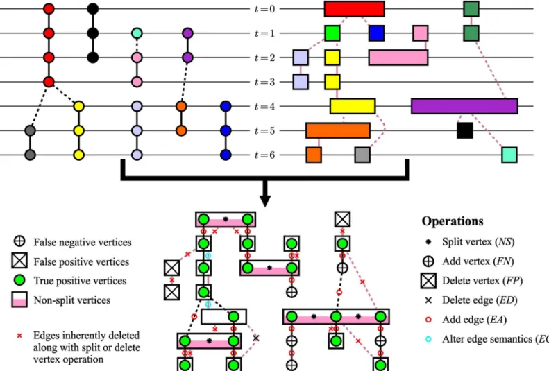
With the assumption of non-negative weights along with at least one weight being positive, theAOGMmeasure is bounded below by zero. Its value is equal to zero when a computed graph is identical to the ground-truth reference or when it contains only errors penalized with a zero weight. TheAOGMvalue increases, theoretically to infinity, with the increasing com-plexity of the transformation that converts the computed graph into the reference one, where complexity is judged with respect to operations penalized with non-zero weights. The higher theAOGMvalue is, the worse output an algorithm has provided and the worse its ranking is. An example of calculating theAOGMmeasure is illustrated inFig 2.
The ability of an algorithm to detect all important objects can be measured using theAOGM
measure when keeping only vertex-related weights positive (i.e.,wNS,wFN,wFP>0;wED=wEA=
wEC= 0). We further refer to such variant of theAOGMmeasure asAOGM-D. Analogously, when keeping only the edge-related weights positive (i.e.,wNS=wFN=wFP= 0;wED,wEA,wEC> 0), theAOGMmeasure evaluates the ability of an algorithm to follow objects in time (i.e., its asso-ciation skills). We further refer to such variant of theAOGMmeasure asAOGM-A.
Results and Discussion
Measure minimality
The computation of theAOGMmeasure is a deterministic procedure, which always returns a sin-gle value derived from the number of differences between the computed and reference graphs. Because we can, thanks to the detection test given byEq (2), uniquely match the graphs, the set of errors is also unique and can be easily determined. The allowed graph operations to correct the errors areadd,delete, andsplita vertex andadd,delete, andalter the semanticsof an edge. All but thesplit vertexoperation are independent in a sense that they cannot be substituted by a rea-sonable combination of the others and each operation directly corrects one error. A non-split vertex withmreference vertices assigned could also be corrected using the following sequence of operations: delete the non-split vertex and addmnew vertices. If the cost of this sequence is Fig 2. An example of calculating theAOGMmeasure for a reference graph (upper left) formed of circular vertices and black edges and a computed graph (upper right) formed of rectangular vertices and dark pink edges.In both graphs, the vertical axis represents the temporal domain and the horizontal axis represents the spatial domain (i.e., each vertex has a certain spatial extent). TheAOGMmeasure is the weighted sum of the following quantities (bottom): the number of splits (NS= 5, black asterisks in pink-white rectangles) computed as the difference between the number of true positive vertices (20 green circles) and the number of white and pink-white rectangles containing at least one green circle (15), the number of false negative vertices (FN= 5, white circles with the black plus sign), the number of false positive vertices (FP= 3, white rectangles with the black cross), the number of redundant edges (ED= 1, black cross), the number of missing edges (EA= 16, small red circles), and finally the number of edges with wrong semantics (EC= 2, small blue circles).
higher than the cost ofm−1split vertexoperations, theAOGMvalue is equal to the minimum
cost necessary to transform the computed graph into the reference one. We formulate the neces-sary condition, which guarantees theAOGMvalue to be not only the weighted sum of the lowest number of graph operations but also the minimum weighted sum, as
wNSðm? 1Þ w
FPþwFNm
? ð13Þ
wherem?is the maximum number of reference vertices assigned to a single non-split vertex among all non-split vertices. For practical purposes, the minimality condition can be weakened towNSwFNto be independent of the input graphs.
Note that the measure prototype used in the first Cell Tracking Challenge calculated the edge-related errors over the entire computed graph and therefore, some of the erroneous edges attached to non-split vertices were inherently corrected along with the vertex splitting while the others were not. This complicated the measure minimality reasoning because the cost of correcting a single non-split vertex may have also involved the penalties for a variable number ofdelete edgeandalter the edge semanticsoperations on the left side ofEq (13)and for a vari-able number ofadd edgeoperations on the right side ofEq (13), and therefore we slightly mod-ified the measure definition. By calculating the edge-related errors over the induced subgraph only, the correction of vertex-related errors is clearly separated from the edge-related ones, allowing minimality condition to be formulated only using the vertex-related weights. In gen-eral, the proposed measure penalizes the splitting errors slightly higher than the measure used in the first Cell Tracking Challenge, in particular due to a slight increase in the number ofadd edgeoperations, being in average approximately 1.88 per non-split vertex, caused by inherent deleting of all edges attached to non-split vertices during their splittings. However, such increase does not have any practical impact on the compiled rankings and they remain unchanged for all algorithms and datasets used in the first Cell Tracking Challenge regardless of the way how the edges attached to non-split vertices are handled.
Testing data
We experimentally validated the proposed measure using the results of four cell tracking algo-rithms (COM-US, HEID-GE, KTH-SE, and PRAG-CZ as named in [22]) that participated in the first Cell Tracking Challenge. These algorithms provided complete tracking results for the entire competition dataset repository [22], which allowed us to study theAOGMmeasure behavior under distinct scenarios involving, in particular, various cell phenotypes (i.e., shape, density, and motion model) and acquisition configurations (i.e., imaging system, image data dimensionality, and time step). The basic properties of the competition datasets are listed in
Table 1. As our primary interest lies in analyzing theAOGMmeasure behavior with respect to the choice of weights inEq (12), rather than in compiling a ranking of the competing algo-rithms and in discussing their strengths and weaknesses, details about the algoalgo-rithms are omit-ted. We further refer to them as A1, A2, A3, and A4 in a random but fixed order.
Distribution of tracking errors
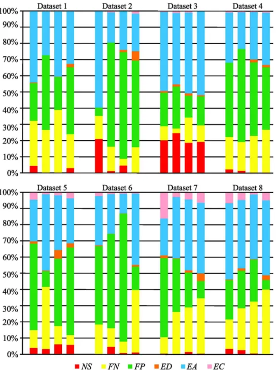
We focused on the statistical analysis of errors in tracking results produced by the four tested algorithms to reveal the distribution of errors under distinct scenarios displayed in the compe-tition datasets (Table 1). The average number and standard deviation of particular errors, nor-malized either per ground-truth vertex or per ground-truth edge to facilitate the comparison between datasets with different numbers of objects, are listed inTable 2. The distribution of errors that the algorithms made in particular datasets is shown inFig 3. The measured values revealed three key observations. First, from the computed standard deviations of errors, it can be observed that the tested algorithms made different types of errors in each particular dataset. Second, there is a preponderance of theadd edgeoperations over theadd vertexones because correcting a false negative vertex requires adding at least one edge to integrate the vertex into a particular track, except when a whole track is formed of a single vertex. Furthermore, missing edges may need to be added also due to inherent deletion of all edges attached to non-split ver-tices. Third, the predominance of a specific error seems to be dataset-dependent: the false nega-tive detection predominates in Datasets 5 and 8, the incorrectly clustered objects in Dataset 3, and the false positive detection in the remaining datasets.
Table 1. Basic properties of the competition repository of diverse fluorescence microscopy datasets analyzed in this work.
Dataset Objects of interest Imaging system Dim. Time step [min] No. of frames No. of series
1 Rat mesenchymal stem cells PerkinElmer Ultraview ERS 2D 20 48 2
2 H157 human lung cancer cells PerkinElmer Ultraview ERS 3D 2 60 2
3 MDA231 breast carcinoma cells Olympus FluoView F1000 3D 80 12 2
4 Nuclei of embryonic stem cells Leica TCS SP5 2D 5 92 2
5 Nuclei of HeLa cells Olympus IX81 2D 30 92 2
6 Nuclei of CHO cells Zeiss LSM 510 3D 9.5 92 2
7 Nuclei of HL60 cells Simulation toolkit 2D 28.8–57.6 56–100 6
8 Nuclei of HL60 cells Simulation toolkit 3D 28.8–57.6 56–100 6
doi:10.1371/journal.pone.0144959.t001
Table 2. The average number and standard deviation of errors in tracking results normalized either per ground-truth vertex or per ground-truth edge depending on a particular error type.The second and third columns list the aggregated numbers of vertices and edges in the ground-truth references per dataset.
Dataset Si|VRi|
S
i|ERi| μNS±σNS μFN±σFN μFP±σFP μED±σED μEA±σEA μEC±σEC
1 915 885 0.017±0.018 0.510±0.267 0.651±0.494 0.011±0.015 0.607±0.229 0.001±0.001
2 490 478 0.012±0.012 0.057±0.069 0.232±0.300 0.003±0.003 0.097±0.076 0.003±0.003
3 846 767 0.159±0.072 0.064±0.030 0.155±0.085 0.010±0.005 0.400±0.102 0.006±0.005
4 5432 5364 0.009±0.011 0.142±0.125 0.385±0.445 0.003±0.003 0.185±0.160 0.002±0.002
5 29374 29136 0.012±0.011 0.095±0.148 0.059±0.019 0.004±0.003 0.132±0.174 0.004±0.002
6 1993 1968 0.010±0.014 0.059±0.027 0.222±0.167 0.001±0.001 0.097±0.052 0.002±0.001
7 11741 11617 0.001±0.001 0.035±0.031 0.039±0.040 0.001±0.001 0.052±0.045 0.005±0.002
8 12286 12164 0.002±0.001 0.059±0.059 0.045±0.049 0.002±0.001 0.080±0.070 0.004±0.001
Total 63077 62379 0.028±0.053 0.128±0.181 0.223±0.312 0.004±0.007 0.206±0.218 0.003±0.003
Sensitivity to the choice of weights
We investigated the behavior of theAOGMmeasure with respect to the choice of weights inEq (12). As a reference weight configuration, we adopted the weights used in the first Cell Track-ing Challenge, which reflected the effort needed to correct a particular error manually:wNS= 5 forvertex splitting,wFN= 10 forvertex adding,wFP= 1 forvertex deleting,wED= 1 foredge Fig 3. The distribution of errors committed by the four tested algorithms for individual datasets.Each group of four horizontal bars corresponds to the tested algorithms depicted in the same order for each dataset.
deleting,wEA= 1.5 foredge adding, andwEC= 1 foraltering the edge semantics. Note that such weight configuration satisfies the minimality condition given byEq (13)for anym?.
We wanted to know how a change in the setting of weights would have affected the refer-ence rankings of the four tested algorithms in terms of tracking ability. To this end, we com-puted sectors in weight space leading to the same rankings. The analysis was carried out with respect to the pair of the two most influential weights,wNSandwFN. The other weights were fixed at their original values, serving as normalization factors. By solving systems of linear inequalities in two unknown weights,w
NSandw
FN, within the rectangular domainh0, 10i× h0, 20i, we studied how many transpositions in the obtained rankings occurred, compared to those compiled for the reference configurationðw
NS;w
FNÞ ¼ ð5;10Þ. The domain was chosen
to range from 0 up to a double magnitude of the reference weight in each axis, being centered at the reference weight configuration. Due to the linearity ofEq (12), the solutions of these sys-tems form polygonal sectors, each consisting of the configurations leading to the same ranking. The results for all datasets are shown inFig 4. The borderlines between the sectors correspond to the configurations, for which at least two algorithms gained the sameAOGMvalue. Almost all tested configurations led to no more than one transposition in the reference rankings, and Fig 4. Pairwise disjoint sectors of all possible configurationsðw
NS;w
FNÞwithin the rectangular domain h0, 10i×h0, 20i, which simultaneously preserve a particular ranking for each individual dataset.The red crosses mark the reference configurationðw
NS;w
FNÞ ¼ ð5;10Þused for compiling the reference rankings. The upper-right corners outlined by the white lines consist of the configurations, which break the minimality condition given byEq (13). The colors encode the numbers of transpositions in the particular rankings compared to the reference ones. No transposition occurs in the pink regions, one transposition occurs in the blue regions, and two transpositions occur in the tiny yellow region.
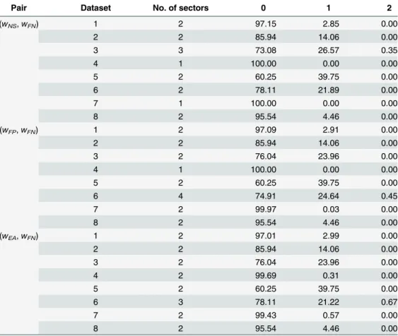
even in the half of the datasets, we observed practically no changes in the reference rankings. We also carried out a similar study for another two pairs of weights, namely (wFP,wFN) and (wEA,wFN), which turned out to be the weights of most frequent errors across all the datasets. The number of sectors and their relative areas are listed inTable 3. Note that in all of the cases the largest sector was formed of the configurations leading to the reference ranking. The sectors with no more than one transposition occupied the whole studied domain in all but three cases. However, in these three cases, they covered more than 99% of the domain.
Based on the information depicted inFig 4andTable 3, it can be concluded that rankings of the tested algorithms compiled using theAOGMmeasure are highly robust against small changes in the choice of weights. This demonstrates that the reference configuration
ðw
NS;w
FNÞ ¼ ð5;10Þcompiles the predominant rankings of the tested algorithms for diverse
datasets (Table 1) because it belongs to the sectors of the largest area (the pink sectors inFig 4, and the column 0 inTable 3).
Comparison with human expert appraisal
To validate theAOGMmeasure against human expert appraisal, we asked three independent human experts to rank the algorithms according to two criteria, which were formulated as (1) Table 3. The number of sectors with different rankings and their relative areas within the rectangular domain centered at the reference weight configuration for individual datasets.The results for three dif-ferent pairs of weights, (wNS,wFN), (wFP,wFN), and (wEA,wFN), are presented. The columns 0, 1, and 2 con-tain the relative areas of the sectors with the particular number of transpositions given by the column label.
Pair Dataset No. of sectors 0 1 2
(wNS,wFN) 1 2 97.15 2.85 0.00
2 2 85.94 14.06 0.00
3 3 73.08 26.57 0.35
4 1 100.00 0.00 0.00
5 2 60.25 39.75 0.00
6 2 78.11 21.89 0.00
7 1 100.00 0.00 0.00
8 2 95.54 4.46 0.00
(wFP,wFN) 1 2 97.09 2.91 0.00
2 2 85.94 14.06 0.00
3 2 76.04 23.96 0.00
4 1 100.00 0.00 0.00
5 2 60.25 39.75 0.00
6 4 74.91 24.64 0.45
7 2 99.97 0.03 0.00
8 2 95.54 4.46 0.00
(wEA,wFN) 1 2 97.01 2.99 0.00
2 2 85.94 14.06 0.00
3 2 76.04 23.96 0.00
4 2 99.69 0.31 0.00
5 2 60.25 39.75 0.00
6 3 78.11 21.22 0.67
7 2 99.43 0.57 0.00
8 2 95.54 4.46 0.00
“the ability of the algorithm to detect all important objects”, shortly detection performance, and (2)“the ability of the algorithm to follow objects in time”, shortly association performance. We did not provide any special instructions on how the experts were supposed to rank the algorithms and we let their decision completely on their opinion. In particular, we did not pro-vide them with the ground truth and did not require any quantification, because it would tend toward the manual counting of errors in the results, which is basically what theAOGM mea-sure does automatically, provided the ground truth exists. The experts allocated points to the algorithms from 0 to 3 (3 means the best) for detection and association separately and the total score in each category was computed by summing up the points. The overall score was obtained by pure addition of the total score in each category.
The rankings compiled usingAOGM-DandAOGM-Avariants of theAOGMmeasure were compared with human expert rankings on all the six real 2-D sequences. The results are sum-marized in Tables4,5and6. They indicate high correlation, with the Kendall rank correlation coefficientτranging from 0.78 up to 0.83, between the rankings on the basis of the proposed
method and human expert opinions. The perfect agreement occurred for three analyzed sequences (Dataset 1/Sequence 1, Dataset 1/Sequence 2, and Dataset 4/Sequence 2).
The difference in the rankings for Dataset 4/Sequence 1 exists because the human experts preponderated the existence of non-split objects and false positive objects over the existence of false negative objects during the evaluation process. Tables7and8show that theAOGM mea-sure could have compiled the same ranking as that compiled by the human experts if their Table 4. The detection ranking comparison of the four tested algorithms (A1–A4) with human expert
appraisal on real 2-D dataset sequences usingAOGM-Dwith weightswNS= 5,wFN= 10,wFP= 1;wED=
wEA=wEC= 0.The black bullets mark the matches in the rankings.
Dataset/ Sequence
AOGM-D Ranking Expert points Ranking
A1 A2 A3 A4 A1 A2 A3 A4 A1 A2 A3 A4 A1 A2 A3 A4
1/1 1415 6376 4977 2879 1 4 3 2 9 0 4 5 •1 •4 •3 •2
1/2 420 2599 1748 963 1 4 3 2 8 0 3 7 •1 •4 •3 •2
4/1 2101 10125 2998 3870 1 4 2 3 4 0 9 5 3 •4 1 2
4/2 1311 16342 1589 1806 1 4 2 3 9 0 6 3 •1 •4 •2 •3
5/1 2281 57113 4785 1587 2 4 3 1 9 0 4 5 1 •4 •3 2
5/2 1813 52985 3244 2095 1 4 3 2 8 0 6 4 •1 •4 2 3
doi:10.1371/journal.pone.0144959.t004
Table 5. The association ranking comparison of the four tested algorithms (A1–A4) with human expert
appraisal on real 2-D dataset sequences usingAOGM-Awith weightswNS=wFN=wFP= 0;wED= 1,
wEA= 1.5,wEC= 1.The black bullets mark the matches in the rankings.
Dataset/ Sequence
AOGM-A Ranking Expert points Ranking
A1 A2 A3 A4 A1 A2 A3 A4 A1 A2 A3 A4 A1 A2 A3 A4
1/1 274.5 889.0 738.5 551.0 1 4 3 2 9 1 2 6 •1 •4 •3 •2
1/2 98.5 280.0 257.0 177.5 1 4 3 2 9 0 4 5 •1 •4 •3 •2
4/1 364.5 1629.0 511.0 612.0 1 4 2 3 5 0 9 4 2 •4 1 •3
4/2 255.0 2105.5 258.5 319.5 1 4 2 3 8 0 7 3 •1 •4 •2 •3
5/1 479.5 9517.5 1141.0 452.5 2 4 3 1 9 0 4 5 1 •4 •3 2
5/2 499.0 9703.5 1334.0 753.5 1 4 3 2 8 0 6 4 •1 •4 2 3
preference on the type of errors was reflected in the weights. The same observation holds for Dataset 5/Sequence 1. Similarly, the swap inAOGM-Afor Dataset 4/Sequence 1 exists because
AOGM-Aputs more emphasis on the missing edges rather than on their semantics. If the weights were accordingly altered, we could have obtained the human expert ranking. In Dataset 5/Sequence 2, A3 was slightly worse than A4 with respect to all types of errors. However, the human experts ranked this algorithm higher. We suppose it is because the human expert com-parison was sometimes very difficult and subjective, especially if the algorithms behaved Table 6. The overall ranking comparison of the four tested algorithms (A1–A4) with human expert appraisal in terms of detection on real 2-D
data-set sequences usingAOGMwith weightswNS= 5,wFN= 10,wFP= 1;wED= 1,wEA= 1.5,wEC= 1.The overall AOGM values and expert points were
obtained by pure addition of the respective quantities for the detection (Table 4) and association (Table 5) parts. The black bullets mark the matches in the rankings.
Dataset/Sequence AOGM Ranking Expert points Ranking
A1 A2 A3 A4 A1 A2 A3 A4 A1 A2 A3 A4 A1 A2 A3 A4
1/1 1689.5 7265.0 5715.5 3430.0 1 4 3 2 18 1 6 11 •1 •4 •3 •2
1/2 518.5 2879.0 2005.0 1140.5 1 4 3 2 17 0 7 12 •1 •4 •3 •2
4/1 2465.5 11754.0 3509.0 4482.0 1 4 2 3 9 0 18 9 2 •4 1 •3
4/2 1566.0 18447.5 1847.5 2125.5 1 4 2 3 17 0 13 6 •1 •4 •2 •3
5/1 2760.5 66630.5 5926.0 2039.5 2 4 3 1 18 0 8 10 1 •4 •3 2
5/2 2312.0 62688.5 4578.0 2848.5 1 4 3 2 16 0 12 8 •1 •4 2 3
doi:10.1371/journal.pone.0144959.t006
Table 7. The ranking comparison of the four tested algorithms (A1–A4) with human expert appraisal in terms of detection on real 2-D dataset
sequences usingAOGM-Dwith weightswNS= 10,wFN= 1,wFP= 10;wED=wEA=wEC= 0.The black bullets mark the matches in the rankings.
Dataset/Sequence AOGM-D Ranking Expert points Ranking
A1 A2 A3 A4 A1 A2 A3 A4 A1 A2 A3 A4 A1 A2 A3 A4
1/1 1354 5548 2448 5273 1 4 2 3 9 0 4 5 •1 •4 3 2
1/2 335 8467 1541 1352 1 4 3 2 8 0 3 7 •1 •4 •3 •2
4/1 4867 29954 4339 4743 3 4 1 2 4 0 9 5 •3 •4 •1 •2
4/2 1759 36279 3711 2873 1 4 3 2 9 0 6 3 •1 •4 2 3
5/1 2926 20456 9519 5035 1 4 3 2 9 0 4 5 •1 •4 •3 •2
5/2 10100 24655 11619 10381 1 4 3 2 8 0 6 4 •1 •4 2 3
doi:10.1371/journal.pone.0144959.t007
Table 8. The overall ranking comparison of the four tested algorithms (A1–A4) with human expert appraisal on real 2-D dataset sequences using
AOGMwith weightswNS= 10,wFN= 1,wFP= 10;wED= 1,wEA= 1.5,wEC= 1.The overall AOGM values and expert points were obtained by pure addition
of the respective quantities for the detection (Table 7) and association (Table 5) parts. The black bullets mark the matches in the rankings.
Dataset/Sequence AOGM Ranking Expert points Ranking
A1 A2 A3 A4 A1 A2 A3 A4 A1 A2 A3 A4 A1 A2 A3 A4
1/1 1628.5 6437.0 3186.5 5824.0 1 4 2 3 18 1 6 11 •1 •4 3 2
1/2 433.5 8747.0 1798.0 1529.5 1 4 3 2 17 0 7 12 •1 •4 •3 •2
4/1 5231.5 31583.0 4850.0 5355.0 2 4 1 3 9 0 18 9 •2 •4 •1 •3
4/2 2014.0 38384.5 3969.5 3192.5 1 4 3 2 17 0 13 6 •1 •4 2 3
5/1 3405.5 29973.5 10660.0 5487.5 1 4 3 2 18 0 8 10 •1 •4 •3 •2
5/2 10599.0 34358.5 12953.0 11134.5 1 4 3 2 16 0 12 8 •1 •4 2 3
similarly, and it was impracticable to manually compute the precise number of errors due to image data complexity (e.g., Dataset 5 contains hundreds of cells per frame).
The experiments demonstrate thatAOGMmeasure can compile expected ranking, being strongly correlated with human expert one, provided the weights reflect the importance of a particular type of error.
Size of ground truth
Typical cell tracking experiments produce hundreds to thousands of 2-D or 3-D images. A decision on what algorithm to use and how to optimally set its parameters is often not an easy task.
A widely adopted approach is to run several algorithms with different parameter settings and visually compare their results. The size of image data often makes such evaluation practica-ble on its limited subset only, although being tricky, especially for 3-D experiments, and subjec-tive due to inter-operator variability and a graphical user interface used.
An alternative approach is to create ground truth for a part of image data and use the
AOGMmeasure for objective and accurate evaluation of the algorithms. In general, the crea-tion of ground truth is laborious, although the amount of work can be reduced by adopting an edit-based framework [23]. Nevertheless, such effort pays off soon when multiple algorithms need to be evaluated and their parameters optimally tuned.
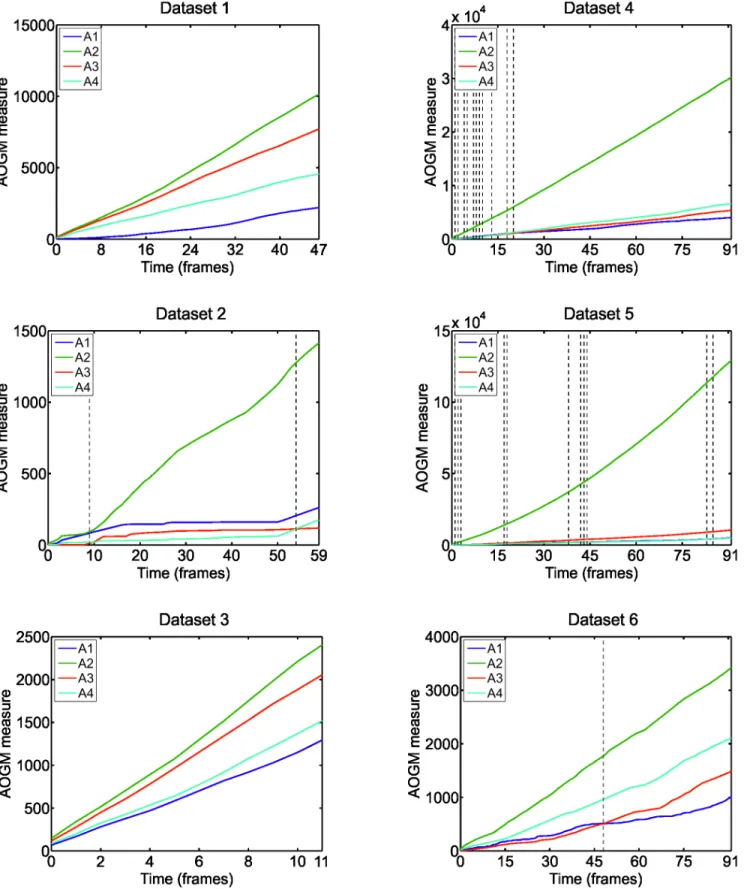
However, any general recommendation on the size of ground truth to get unbiased evalua-tion of the algorithm performance can be hardly stated. It depends on the complexity of image data and particular application. Instead, we computed the temporal evolution of theAOGM
measure for each algorithm and each real dataset (Fig 5). It can be observed that the number of frames after which the rankings of the tested algorithms stabilized varied across the datasets. It can also be observed often a linear increase in theAOGMvalue, indicating the tested algo-rithms committed approximately the same number of errors over time.
Conclusions
In this paper, theAOGMmeasure, an accuracy measure for objective and systematic compari-son of cell tracking algorithms that are capable of providing segmentation of individual cells rather than simplifying them as single-point objects, has been defined and analyzed. Treating tracking results as an acyclic oriented graph, the proposed measure assesses how difficult it is to transform a computed graph into a given ground-truth graph. The cost of such a transfor-mation is defined as the weighted sum of the lowest number of graph operations needed to make the graphs identical. The behavior of theAOGMmeasure was analyzed on tracking results provided by four state-of-the-art cell tracking algorithms that participated in the first Cell Tracking Challenge. The performed analyses verified its robustness and stability against small changes in the choice of weights for diverse fluorescence microscopy datasets.
Fig 5. The temporal evolution of theAOGMmeasure, averaged over the two sequences per each real dataset, for the four tested algorithms (A1– A4).The dashed vertical lines indicate the frames at which the algorithm ranking compiled using theAOGMmeasure has changed.
In addition to being robust, stable, and flexible, theAOGMmeasure is also universal. The measure penalizes all possible errors in tracking results, not concentrating on only a single, often application-limited aspect of cell tracking as the existing approaches do [4,16,17]. It can be applied to datasets with various characteristics, even nearly degenerated cases such as those showing no division or containing only a single cell. Furthermore, it can be used for evaluating the performance of any cell tracking algorithm irrespective of its nature because it evaluates its final output. Therefore, developers can use theAOGMmeasure to easily compare the perfor-mance of a cell tracking algorithm under development to that of existing algorithms, whereas analysts can use it to determine the optimal parameters of a chosen algorithm for a dataset to be analyzed. The software for computing theAOGMmeasure is made publicly available at
http://cbia.fi.muni.cz/aogm/or as a supplementary materialS1 Software, free of charge for noncommercial and research purposes.
Supporting Information
S1 Software. AOGMMeasure.This package contains a routine for computing the AOGM measure.
(ZIP)
S1 File. Supporting Information File.This supporting information file contains all relevant data used for generating the results described in the manuscript.
(XLSX)
Author Contributions
Conceived and designed the experiments: Pavel Matula MM DVS Petr Matula. Performed the experiments: Pavel Matula MM. Analyzed the data: Pavel Matula MM. Wrote the paper: Pavel Matula MM DVS Petr Matula COS MK.
References
1. Meijering E, Dzyubachyk O, Smal I, Cappellen WA. Tracking in Cell and Developmental Biology. Semi-nars in Cell and Developmental Biology. 2009; 20(8):894–902. doi:10.1016/j.semcdb.2009.07.004
PMID:19660567
2. Zimmer C, Zhang B, Dufour A, Thébaud A, Berlemont S, Meas-Yedid V, et al. On the Digital Trail of Mobile Cells. IEEE Signal Processing Magazine. 2006; 23(3):54–62. doi:10.1109/MSP.2006.1628878 3. Ananthakrishnan R, Ehrlicher A. The Forces Behind Cell Movement. International Journal of Biological
Sciences. 2007; 3(5):303–317. doi:10.7150/ijbs.3.303PMID:17589565
4. Li K, Chen M, Kanade T, Miller ED, Weiss LE, Campbella PG. Cell Population Tracking and Lineage Construction with Spatiotemporal Context. Medical Image Analysis. 2008; 12(5):546–566. doi:10.
1016/j.media.2008.06.001PMID:18656418
5. Al-Kofahi O, Radke RJ, Goderie SK, Shen Q, Temple S, Roysam B. Automated Cell Lineage Construc-tion: A Rapid Method to Analyze Clonal Development Established with Murine Neural Progenitor Cells. Cell Cycle. 2006; 5(3):327–335. doi:10.4161/cc.5.3.2426PMID:16434878
6. Harder N, Batra R, Diessl N, Gogolin S, Eils R, Westermann F, et al. Large-Scale Tracking and Classifi-cation for Automatic Analysis of Cell Migration and Proliferation, and Experimental Optimization of High-Throughput Screens of Neuroblastoma Cells. Cytometry Part A. 2015; 87(6):524–540. doi:10.
1002/cyto.a.22632
7. Li F, Zhou X, Ma J, Wong STC. Multiple Nuclei Tracking Using Integer Programming for Quantitative Cancer Cell Cycle Analysis. IEEE Transactions on Medical Imaging. 2010; 29(1):96–105. doi:10.1109/
TMI.2009.2027813PMID:19643704
8. Magnusson KEG, Jaldén J, Gilbert PM, Blau HM. Global Linking of Cell Tracks Using the Viterbi Algo-rithm. IEEE Transactions on Medical Imaging. 2015; 34(4):911–929. doi:10.1109/TMI.2014.2370951
9. Padfield D, Rittscher J, Roysam B. Coupled Minimum-Cost Flow Cell Tracking for High-Throughput Quantitative Analysis. Medical Image Analysis. 2011; 15(1):650–668. doi:10.1016/j.media.2010.07.
006PMID:20864383
10. Dufour A, Thibeaux R, Labruyère E, Guillén N, Olivo-Marin JC. 3-D Active Meshes: Fast Discrete Deformable Models for Cell Tracking in 3-D Time-Lapse Microscopy. IEEE Transactions on Image Pro-cessing. 2011; 20(7):1925–1937. doi:10.1109/TIP.2010.2099125PMID:21193379
11. Dzyubachyk O, van Cappellen WA, Essers J, Niessen WJ, Meijering E. Advanced Level-Set-Based Cell Tracking in Time-Lapse Fluorescence Microscopy. IEEE Transactions on Medical Imaging. 2010; 29(3):852–867. doi:10.1109/TMI.2009.2038693PMID:20199920
12. Maška M, Daněk O, Garasa S, Rouzaut A, Muñoz-Barrutia A, Ortiz-de-Solórzano C. Segmentation and Shape Tracking of Whole Fluorescent Cells Based on the Chan-Vese Model. IEEE Transactions on Medical Imaging. 2013; 32(6):995–1006. doi:10.1109/TMI.2013.2243463PMID:23372077
13. Padfield D, Rittscher J, Thomas N, Roysam B. Spatio-Temporal Cell Cycle Phase Analysis Using Level Sets and Fast Marching Methods. Medical Image Analysis. 2009; 13(1):143–155. doi:10.1016/j.media.
2008.06.018PMID:18752984
14. Bergeest JP, Rohr K. Efficient Globally Optimal Segmentation of Cells in Fluorescence Microscopy Images Using Level Sets and Convex Energy Functionals. Medical Image Analysis. 2012; 16(7):1436–
1444. doi:10.1016/j.media.2012.05.012PMID:22795525
15. Stegmaier J, Otte JC, Kobitski A, Bartschat A, Garcia A, Nienhaus GU, et al. Fast Segmentation of Stained Nuclei in Terabyte-Scale, Time Resolved 3D Microscopy Image Stacks. PLoS ONE. 2014; 9 (2):e90036. doi:10.1371/journal.pone.0090036PMID:24587204
16. Kan A, Chakravorty R, Bailey J, Leckie C, Markhami J, Dowling MR. Automated and Semi-Automated Cell Tracking: Addressing Portability Challenges. Journal of Microscopy. 2011; 244(2):194–213. doi:
10.1111/j.1365-2818.2011.03529.xPMID:21895653
17. Degerman J, Thorlin T, Faijerson J, Althoff K, Eriksson PS, Put RVD, et al. An Automatic System forin vitroCell Migration Studies. Journal of Microscopy. 2009; 233(1):178–191. doi:10.1111/j.1365-2818.
2008.03108.xPMID:19196424
18. Kasturi R, Goldgof D, Soundararajan P, Manohar V, Garofolo J, Bowers R, et al. Framework for Perfor-mance Evaluation of Face, Text, and Vehicle Detection and Tracking in Video: Data, Metrics, and Pro-tocol. IEEE Transactions on Pattern Analysis and Machine Intelligence. 2009; 31(2):319–336. doi:10.
1109/TPAMI.2008.57PMID:19110496
19. Chenouard N, Smal I, de Chaumont F, Maška M, Sbalzarini IF, Gong Y, et al. Objective Comparison of
Particle Tracking Methods. Nature Methods. 2014; 11(3):281–289. doi:10.1038/nmeth.2808PMID:
24441936
20. Kan A, Leckie C, Bailey J, Markham J, Chakravorty R. Measures for Ranking Cell Trackers Without Manual Validation. Pattern Recognition. 2013; 46(11):2849–2859. doi:10.1016/j.patcog.2013.04.007 21. Kan A, Markham J, Chakravorty R, Bailey J, Leckie C. Ranking Cell Tracking Systems Without Manual
Validation. Pattern Recognition Letters. 2015; 53(1):38–43. doi:10.1016/j.patrec.2014.11.005 22. Maška M, Ulman V, Svoboda D, Matula P, Matula P, Ederra C, et al. A Benchmark for Comparison of
Cell Tracking Algorithms. Bioinformatics. 2014; 30(11):1609–1617. doi:10.1093/bioinformatics/btu080
PMID:24526711
23. Winter M, Wait E, Roysam B, Goderie SK, Ali RAN, Kokovay E, et al. Vertebrate Neural Stem Cell Seg-mentation, Tracking and Lineaging with Validation and Editing. Nature Protocols. 2011; 6(12):1942–
1952. doi:10.1038/nprot.2011.422PMID:22094730
24. Svoboda D, Kozubek M, Stejskal S. Generation of Digital Phantoms of Cell Nuclei and Simulation of Image Formation in 3D Image Cytometry. Cytometry Part A. 2009; 75A(6):494–509. doi:10.1002/cyto.
a.20714
25. Svoboda D, Ulman V. Generation of Synthetic Image Datasets for Time-Lapse Fluorescence Micros-copy. In: Proceedings of the 9th International Conference on Image Analysis and Recognition; 2012. p. 473–482.
26. Smal I, Draegestein K, Galjart N, Niessen W, Meijering E. Particle Filtering for Multiple Object Tracking in Dynamic Fluorescence Microscopy Images: Application to Microtubule Growth Analysis. IEEE Transactions on Medical Imaging. 2008; 27(6):789–804. doi:10.1109/TMI.2008.916964PMID:
18541486
27. Huth J, Buchholz M, Kraus JM, Schmucker M, von Wichert G, Krndija D, et al. Significantly Improved Precision of Cell Migration Analysis in Time-Lapse Video Microscopy Through Use of a Fully Auto-mated Tracking System. BMC Cell Biology. 2010; 11:24. doi:10.1186/1471-2121-11-24PMID: