Article
Complex dynamics of a stochastic discrete modified Leslie-Gower
predator-prey model with Michaelis-Menten type prey harvesting
A. Elhassanein
Dept. of Math., Faculty of Science, Damanhour University, Damanhour, Egypt E-mail: [email protected]
Received 30 January 2014; Accepted 5 March 2014; Published online 1 June 2014
Abstract
This paper introduced a stochastic discretized version of the modified Leslie-Gower predator-prey model with Michaelis-Menten type prey harvesting. The dynamical behavior of the proposed model was investigated. The
existence and stability of the equilibria of the skeleton were studied. Numerical simulations were employed to show the model's complex dynamics by means of the largest Lyapunov exponents, bifurcations, time series diagrams and phase portraits. The effects of noise intensity on its dynamics and the intermittency phenomenon
were also discussed via simulation.
Keywords ecosystems; Leslie-Gower predator-prey model; skeleton; bifurcations; chaos.
1 Introduction
Deterministic nonlinear predator-prey models (ODE models) are widely used to understand the dynamics of the ecosystems (Rosenzweig and MacArthur, 1963; Clark, 1976; Steven, 1994; Srinivasu, 2001; Kondoh, 2003; Murdoch et al., 2003; Nedorezov and Sadykov, 2012). In recent years, there has been an increasing interest in
Leslie-Gower type predator-prey model (Hsu and Huang, 1995; Li and Xiao, 2007; Liang and Pan, 2007; Song et al., 2009; Tian and Weng, 2011; Tian and Zhu, 2012). The local and global stability for a predator-prey
model of modified Leslie-Gower and Holling-type II with time-delay has been considered by Lin and Ho (2006). Bifurcation analysis of a Leslie-Gower prey-predator model with Holling-type III functional response has been studied by Li and Xiao (2007). The global stability of a Leslie-Gower prey-predator model with
proportional harvesting in both prey and predator has been studied by Zhang et al. (2011). By defining a suitable Lyapunov function, the global stability of the unique interior equilibrium of the system was shown,
which means that suitable harvesting has no influence on the persistent property of the harvesting system. Mena-Lorca et al. (2007) studied the dynamics of the Leslie-Gower model subjected to the Allee effect with proportionate harvesting. The dynamical behavior of the periodic prey-predator model with a modified
Leslie-Gower Holling-type II scheme and impulsive effect has been studied by Song and Li (2008). Phase portraits Computational Ecology and Software
ISSN 2220721X
URL: http://www.iaees.org/publications/journals/ces/onlineversion.asp RSS: http://www.iaees.org/publications/journals/ces/rss.xml
Email: [email protected] EditorinChief: WenJun Zhang
near the interior equilibria of a Leslie-Gower model with constant harvesting in prey has been considered by Zhu and Lan (2010). Gupta and Chandra (2013) introduced a modified version of the Leslie-Gower
prey-predator model with Holling-type II functional response in the presence of nonlinear harvesting in prey. Many authors (Agarwal, 2000; Agarwal, 1997; Freedman, 1980; Murray, 1989) have argued that the discrete time models governed by difference equations are more appropriate than the continuous ones when the populations
have nonoverlapping generations. Discrete time models can also provide efficient computational models of continuous models for numerical simulations. Discrete Leslie-Gower predator-prey model has also been
studied by many authors. Huo and Li (2004) considered a discrete Leslie-Gower predator-prey model. They obtained sufficient conditions which guarantee the permanence of the model. Under the assumption that the coefficients in the model are periodic, the existence of periodic solution is also obtained. Agiza et al (2009)
investigated discrete-time prey-predator model with Holling type II. The existence and stability of three fixed points have been analyzed. The bifurcation diagrams, phase portraits and Lyapunov exponents have been
obtained for different parameters of the model. The fractal dimension of a strange attractor of the model has been also calculated. They showed that the discrete model exhibits rich dynamics compared with the continuous model. It has been shown that for the discrete-time prey-predator models the dynamics can produce
a much richer set of patterns than those observed in continuous-time models, see Danca (1997), Jing and Yang (2006), Liu and Xiao (2007). The main objective of this paper is to propose a stochastic discrete version of the
modified Leslie-Gower predator-prey model with Michaelis-Menten type prey harvesting, and analyze its chaotic behavior.
The organization of this paper is as follows. In section 2, a stochastic discrete version of the modified Leslie-Gower predator-prey model with Michaelis-Menten type prey harvesting is formulated. In section 3, the stability condition of the system are derived. The simulation is used in section 4, to discuss the analytical
results and to show the effects of noise intensity on the dynamics of the system.
2 The Stochastic Discrete Model
In the case of continuous time the modified Leslie-Gower predator-prey model with Michaelis-Menten type prey harvesting has the following form
,
(2.1)
here, and are the prey and predator population densities respectively and are intrinsic
growth rate and environmental carrying capacity for the prey species respectively. is the maximum value
of the per capita reduction rate of prey, measures the extent to which the environment provides protection
to prey and predator (under the assumption that the extent to which the environment provides protection to
both the predator and prey is the same (Ji et al., 2009, 2011), measures the growth rate of the predator
species, is the maximum value of the per capita reduction rate of predator, is the catchability coefficient,
is the effort applied to harvest the prey species, and , and are suitable constants. All the parameters
are assumed to be positive due to biological considerations.
Using a suitable non-dimensional scheme, the system (2.1) can be transformed into the following system, Gupta and Chandra (2013).
,
with the initial conditions, , where , , , , , and are all positive.
Applying the forward Euler scheme to model (2.2) we obtain the following stochastic discrete modified Leslie-Gower predator-prey model with Michaelis-Menten type prey harvesting model
,
(2.3)
where is the step size , , , , , and are defined as model (2.2) and ( , ) are assumed to be an
i.i.d. white noise sequence conditional upon the history of the time series, which is denoted Ω
, that is, , \Ω and \Ω \Ω , and is a scalar
parameter of the noise intensity.
3 The Skeleton (Free Noise System)
In this section we study the chaotic behaviour of the free noise system (2.3) caused by the change of time step.
Where , the system (2.3) becomes
,
(3.1)
Fixed points of the system (3.1) are derived in the following.
Lemma 3.1. The fixed points of the system (3.1), are
, ;
, , where
, and
, , where ,
Proof. The fixed points of the system (3.1) are obtained as the solution of the algebraic system:
,
which is obtained by setting and in (3.1), it is easy to complete the proof.
The local stability analysis of the system (3.1) can be studied by computing the variation matrix
corresponding to each fixed point. The variation matrix of the system at state variable is given by
, . (3.2)
Theorem 3.1. The fixed point is unstable fixed point for all parameters values.
Proof. In order to prove this result, we estimate the eigenvalues of Jacobian matrix at . The Jacobian
matrix for is
.
the proof is completed.
Theorem 3.2. The fixed point , , is locally asymptotically stable if one of the following conditions is satisfied:
max , max , , max , ;
max , max , min , min , ;
max , max , min , min , ;
min , min , , min ,
otherwise it is unstable fixed point, where , , , ,
, , , , and .
Proof. The Jacobian matrix (3.2) at , , has the form
.
where , and .
The corresponding characteristic equation of matrix , , is
,
where and
If the eigenvalues of the Jacobian matrix of a fixed point are inside the unit circle of the complex plan,
interior fixed point is local stable. Using Jury's conditions (Chatterjee and Yilmaz, 1992; Zhu and Lan, 2010),
we have necessary and sufficient condition for local stability of interior fixed point which are the necessary
and sufficient condition for , , which completes the proof.
4 Numerical Simulation 4.1 Deterministic system
The main purpose of this subsection is to investigate the qualitative behavior of the solution of the nonlinear
system (3.1). To provide some numerical evidence for its chaotic behavior, we present various numerical
results here to show the chaoticity including its bifurcation diagrams, Lyapunov exponents, and fractal
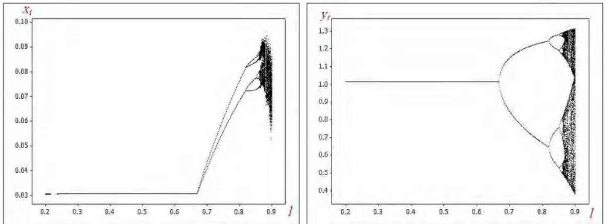
dimension. In Fig. 1(a) bifurcation diagram of the system (3.1) is plotted on the interval . . for
initial point , . , . with , , , , , , , , , . , . In Fig. 2, a plot of the Lyapunov
exponent for attractors of the system (3.1) according to Fig. 1 is presented. A positiveness of this exponent for
. confirms the chaotic character of attractors in this parametrical zone (here, the value
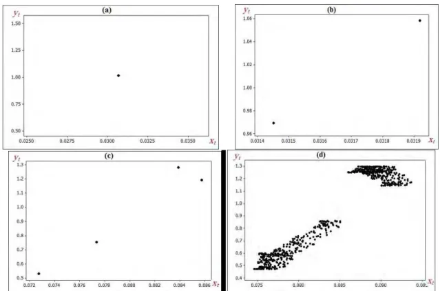
. is a tangent bifurcation point). In Fig. 3 phase portraits are given for different values of to show the
. , . which is attracting point for . . 0 as we can see in Fig. 3. (a). Fig. 3.(b)
show the period-two orbit in the parameter zone 0.6689< l <0.8195. The period-four orbit in the parameter
zone . . is clear in Fig. 3(c). The chaotic attractor for . . is clear in Fig.
3(d). Which means that the system (3.1) undergoes a discrete Hopf bifurcation. One of the commonly used
characteristics for classifying and quantifying the chaoticity of a dynamical system is fractal dimensions,
(Cartwright, 1999; Zhu and Lan, 2010). Via simulation we get two Lyapunov exponents .
. for . , which means that .
. . . There for the system (3.1)
exhibits a fractal structure and its attractor has a fractal dimension which is chaotic behavior.
Fig. 1 Bifurcation diagram of (3.1), for . . and initial point , . , . with
, , , , , , , , , . , .
Fig. 3 Phase portrait of the system (3.1) for: (a) . ; (b) . (c) . (d) . with , , , , , , , , , . , .
4.2 Stochastic model
Along with the deterministic systems (3.1) we consider a stochastic system forced by additive noise (2.3),
where and are uncorrelated Gaussian random processes with parameters , and
, and is a scalar parameter of the noise intensity. We study a behavior of this stochastic model for
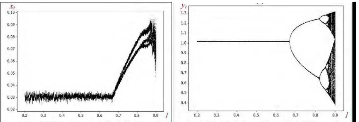
different sets of parameters and . In Figs. 4, 5 and 6, stochastic attractors of the system (2.3) are plotted on
the interval . . for three values of the noise intensity . , . , and . .
Lyapunov exponents corresponding to each value of noise intensity are given in Fig. (7) (a), (b) and (c)
respectively. As we can see, noise deforms the deterministic attractor (compare Figs. 2 and 7). As noise
intensity increases, a border between order and chaos moves to the left. The changes of the arrangement of
attractors are accompanied by the changes in dynamical characteristics (compare Lyapunov exponents in Figs.
2 and 8). The most essential difference between stochastic and deterministic attractors is observed near the
bifurcation point . . The underlying reason is that in the vicinity of this bifurcation point attractors
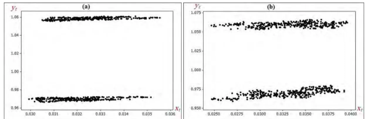
are highly sensitive to random disturbances. Consider in detail a behavior of stochastic system (2.3)
near . . Compare the stochastic response of this system for two fixed values . and
. . Consider . . For low noise . , random states are concentrated near the stable
deterministic equilibrium (see Figs. 8 and 12(a)), they have distribution with mean equal approximately
Σ .. .. .
For . one can see stochastic oscillations of large amplitude. Indeed, as the noise intensity increases,
the dispersion of random states near growsc see Table 1. After these oscillations, iterations come to the
vicinity of the point again and so on (see Figs. 9 and 12(b)). In this case, the stochastic model (2.3)
exhibits a coexistence of two different dynamical regimes even if the system (3.1) has a stable equilibrium
only. This type of dynamics of the system (2.3) can be determined as a noise-induced intermittency
(Bashkirtseva and Ryashko 2013). In Figs. 10 and 11, time series of the stochastic system (2.3) with
. for . and . are plotted. As can be seen, noise-induced intermittency for this
. is observed for the lower noise intensity, see also Fig. 13. For stochastic attractors and their
dynamic characteristics, a dependence on noise level is illustrated in Figs. 14 and 15 for . and
. . In Fig. 14, one can see a sharp growth of the size of the attractor as noise intensity exceeds some
critical value. A change of the sign of Lyapunov exponent from minus to plus can be interpreted as a transition
from regular to noise-induced chaotic regime (see Fig. 16). Thus, the results presented here give us a
qualitative description of noise-induced transitions from the regular regime to intermittency.
Fig. 4 Bifurcation diagrams of the stochastic model (2.3) with . , . . , and , , , , , , , , , . , .
Fig. 6 Bifurcation diagrams of the stochastic model (2.3) with . , . . , and , , , , , , , , , . , .
Fig. 7 Lyapunov exponents of the stochastic model (2.3) with . . : for (a) . ; (b) . ; (c)
. .
Fig. 9 Time series of the stochastic model (2.3) with . , . , , , , , , , , , . , .
Fig. 10 Time series of the stochastic model (2.3) with . , . and , , , , , , , , , . , .
Fig. 11 Time series of the stochastic model (2.3) with . , . and , , , , , , , , , . , .
Fig. 12 Phase portrait of the system (2.3) with . , and , , , , , , , , , . , for: (a) . ;
Fig. 13 Phase portrait of the system (2.3) with . and , , , , , , , , , . , for: (a) . ; (b) . .
Fig. 14 Attractors of the stochastic system (2.3) for . ; . and , , , , ,
, , , , . , .
Fig. 15 Attractors of the stochastic system (2.3) for . ; . , and , , , , ,
, , , , . , .
Fig. 16 Lyapunov exponents of the stochastic system (2.3) with . and
Table 1 Mean of the stochastic states , of the system (2.3) at different values of , and , , , , , , , , , . , .
╲ 0. 0.
0.0002 (0.030572,1.0153) (0.032278,1.0142)
. (0.029719,1.0147) (0.033094,1.0145)
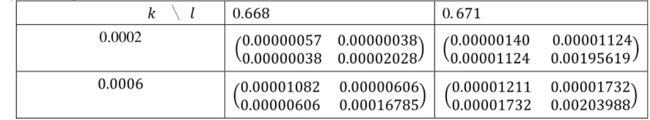
Table 2 Covariance matrices of the stochastic states , of the system (2.3) at different values of , and , , , , , , , , , . , .
╲ 0. 0.
0.0002 . .
. . .. . .
. . .
. . .. ..
5 Conclusion
From a mathematical as well as biological point of view the predator-prey models can be formulated as systems of differential or difference equations (Nedorezov and Sadykov, 2012). The current paper have
proposed a stochastic discrete modified Leslie-Gower predator-prey model with Michaelis-Menten type prey harvesting, where the protection provided by the environment for both the prey and predator is the same. The
model shows rich and varied dynamics. The local stability of fixed points have been discussed. The results show that the origin is unstable equilibrium point of the system. There is a unique interior equilibrium point which is locally stable for certain parametric restrictions. The effectiveness of the time step on the dynamics of
the system has been shown. The chaotic behaviour of the system has been proved. We focus on the study of the noise-induced type-I intermittency phenomenon and chaotization observed near tangent bifurcation. The
remarkable feature of the dynamics of the model considered here is that small noises generate large-amplitude chaotic oscillation.
References
Agarwal RP. 2000. Difference Equations and Inequalities: Theory, Method and Applications. Monographs and Textbooks in Pure and Applied Mathematics (Volume 2). Marcel Dekker, New York, USA
Agarwal RP, Wong PJY. 1997. Advance Topics in Difference Equations. Kluwer, Dordrech. Germany
Agiza HN, ELabbasy EM, EL-Metwally H, Elsadany AA 2009. Chaotic dynamics of a discrete prey-predator model with Holling type II. Nonlinear Analysis, RWA 10: 116-129
Bashkirtseva I, Ryashko L. 2013: Stochastic sensitivity analysis of noise-induced intermittency and transition to chaos in one-dimensional discrete-time systems. Physica A, 392: 295-306
Cartwright J HE 1999. Nonlinear stifiness, Lyapunov exponents, and attractor dimension. Physical Letters A,
264: 298-304
Chatterjee S, Yilmaz M. 1992. Chaos, fractals and statistics. Statistical Science, 7: 49-68
Clark CW 1976. Mathematical Bioeconomics the Optimal Management of Renewable Resources. Wiley, New York
Biological Physics, 23: 11-20
Freedman HI 1980. Deterministic Mathematics Models in Population Ecology. Marcel Dekker, New York,
USA
Gupta RP, Chandra P. 2013. Bifurcation analysis of modified Leslie-Gower predator-prey model with Michaelis--Menten type prey harvesting. Journal of Mathematical Analysis and Applications, 398: 278-295
Hsu SB, Huang TW. 1995. Global stability for a class of predator-prey systems. SIAM Journal of Applied Mathematics, 55: 763-783
Huo H, and Li WT. 2004. Stable periodic solution of the discrete periodic Leslie-Newer predator-prey model. Mathematical and Computer Modelling 40: 261-269
Ji C, Jiang D, Shi N. 2009. Analysis of a predator--prey model with modified Leslie-Gower and Holling-type
II schemes with stochastic perturbation. Journal of Mathematical Analysis and Applications, 359: 482-498 Ji C, Jiang D, Shi N. 2011. A note on a predator--prey model with modified Leslie-Gower and Holling-type II
schemes with stochastic perturbation. Journal of Mathematical Analysis and Applications, 377(1): 435-440 Jing ZJ, Yang J. 2006. Bifurcation and chaos discrete-time predator--prey system. Chaos, Solitons and Fractals,
27, 259-277
Kondoh M 2003. Foraging adaptation and the relationship between food-web complexity and stability. Science, 299: 1388-1391
Li Y, Xiao D. 2007. Bifurcations of a predator-prey system of Holling and Leslie types. Chaos, Solitons and Fractals, 34, 606-620
Liang Z, Pan H. 2007. Qualitative analysis of a ratio-dependent Holling-Tanner model. J. Math. Anal. Appl. 334, 954-964
Lin CM, Ho CP. 2006. Local and global stability for a predator-prey model of modified Leslie-Gower and
Holling-type II with time-delay. Tunghai Science, 8: 33-61
Liu X, Xiao D 2007. Complex dynamic behaviors of a discrete-time predator-prey system. Chaos, Solitons and
Fractals, 32: 80-94
Mena-Lorca J, Gonzalez-Olivares E, Gonzalez-Yanz B. 2007. The Leslie-Gower predator-prey model with Allee effect on prey: a simple model with a rich and interesting dynamics. In: Proceedings of the
International Symposium on Mathematical and Computational Biology BIOMAT 2006 (Mondaini R, ed). 105, 132, E-papers Servios Editoriais Ltda, R' io de Janeiro, Brazil
Murdoch W, Briggs C, Nisbet R. 2003. Consumer-Resource Dynamics. Princeton University Press, New York, USA
Murray J D 1989. Mathematical Biology. Springer-Verlag, New York, USA
Nedorezov LV, Sadykov AM. 2012. About a modification of Rogers model of parasite-host system dynamics. Proceedings of the International Academy of Ecology and Environmental Sciences, 2(1): 41-49
Song Y, Yuan S, Zhang J. 2009. Bifurcation analysis in the delayed Leslie-Gower predator-prey system. Applied Mathematical Modelling, 33: 4049-4061
Rosenzweig ML, MacArthur RH. 1963. Graphical representation and stability conditions of predator--prey
interactions. American Naturalist, 97: 209
Song XY, Li YF. 2008. Dynamic behaviors of the periodic predator-prey model with modified Leslie-Gower
Holling-type II schemes and impulsive effect. Nonlinear Analysis, RWA 9: 64-79
Srinivasu PDN. 2001. Bioeconomics of a renewable resource in presence of a predator. Nonlinear Analysis, RWA 2: 497-506
Tian C, Zhu P. 2012. Existence and asymptotic behavior of solutions for quasilinear parabolic systems. Acta Applicandae Mathematicae. DOI 10.1007/s 10440-012-9701-7
Tian Y, Weng P. 2011. Stability analysis of diffusive predator-prey model with Modified Leslie-Gower and Holling-Type II schemes. Acta Applicandae Mathematicae, 114(3): 173-192
Zhang N, Chen F, Su Q, Wu T. 2011. Dynamic behaviors of a harvesting Leslie-Gower predator-prey model.
Discrete Dynamics in Nature and Society. http://dx.doi.org/10.1155/2011/473-94.
Zhu CR, Lan KQ. 2010. Phase portraits, Hopf-bifurcations and limit cycles of Leslie-Gower predator--prey