On the Dynamics of a General Predator-Prey System

Journal of Mathematics and Statistics 7 (4): 295-301, 2011 ISSN 1549-3644

© 2011 Science Publications

Corresponding Author: M.M.A. El-Sheikh, Department of Mathematics, Faculty of Science, Menoufia University, Sheben El-Koom, Egypt

On the Dynamics of a General Predator-Prey System

1

M.M.A. El-Sheikh,

1,2

S.A.A. El-Marouf and

2

Z.M. Alaofy

1

Department of Mathematics, Faculty of Science,

Menoufia University, Sheben El-Koom, Egypt

2

Department of Mathematics, Faculty of Science,

Taibah University, Saudi Arabia

Abstract: Problem statement: In this study a general two dimensional predator-prey model is considered. The dynamic and existence of equilibrium points are studied.

Conclusion/Recommendations: Hopf bifurcation is discussed. The existence and uniqueness of limit

cycles is proved. Special cases are considered to justify our results.

Key words: Predator-prey system, functional response, limit cycles, hopf bifurcation, mathematics subject classification, analyzing models, interacting species, predator population, efficiency rate

INTRODUCTION

There has been a demanding need for developing and analyzing models of interacting species in ecosystems. Predator-prey models are one of the most important models of two-species interaction. In this study we are concerned with a general 2-dimensional predator-prey system of the form

1 1

2 2

dx

xg(x) yp(x) q E x, dt

dy

Dy syp(x) q E y dt

= − −

= − + −

(1)

where, x and y are the prey and the predator population sizes, respectively. The parameters s, D and k are positive and represent the conversion efficiency rate of prey to predator, predator death rate and the carrying capacity of the prey population, respectively. The parameters E1≥ 0, E2≥ 0denote the harvesting efforts for the predator and prey respectively. The expressions q1E1x and q2E2x represent the catch of the respective species, where q1and q₂ denote the catch ability coefficients of the prey and predator, respectively. The functions g(x) and p(x) denote the functional response of the prey and predator, respectively and satisfy the assumptions p(0) = 0 and g(0)>0, for all x>0. There have been considerable interests in the dynamics of the predator-prey models of some special cases of (1) by several authors (Attili, 2001; Attili and Mallak, 2006; Xiao and

Ruan, 2001; Hesaaraki and Moghadas, 2001; Kar and Matsuda, 2007; Moghadas and Corbett, 2008; Moghadas and Alexander, 2005; Sugie et al., 1997; Ruan and Xiao, 2001). Hasik (2000); Sesay et al. (2010); Moghadas and Alexander (2006); Saha and Bandyopadhyay (2005) and Tao et al. (2011) the authors considered Eq. 1 in the special caseg(x) r(1 x)

k

= −

.

The aim of this study is to discuss the qualitative properties of the general predator-prey system (1). We discuss the existence and stability of equilibria and nonexistence criteria for limit cycles. We explore the uniqueness of limit cycles using Kuang and Freedmann approach (Moghadas and Corbett, 2008) and some applications. It is natural due to biological considerations to expect that the solutions of (1) must to be positive and bounded. So we give the following result which is a partial extension of those of (Freedman and So, 1985) and (Saha and Bandyopadhyay, 2005).The paper end with a brief discussion.

Theorem 1.1: All the solutions of Eq. 1 which start in

2

+

ℝ are positive and uniformly bounded.

1

w(x, y) x y

s

= +

Then we easily obtain:

2

1 1 2

dw dx 1 dy D q

xg(x) q E x y E y

dt = dt+s dt = − −s − s

i.e. for any r, we have:

2

1 1 1

dw

rw x( r q E ) M M ,say

dt + ≤ α + − ≤ =

where, α = max g(x) and x≤_{M =(}α_+r-q1E1).

Thus applying the theory of differential inequality (Freedman and So, 1985), we obtain:

rt rt

1

M

0 w(x, y) (1 e ) w(x(0), y(0))e

r

− −

< < − + .

So the limits as tends to ∞ yields _{0 w(x, y)} M1

r

< < . Thus we have that all solutions of (1) start in 2

+

ℝ are

confirmed to the region D

where_D

( )

_{x, y R : w}2 M1 _{for 0}

r

+

 

= ∈ = + ∈ > 

 

.

_{The equilibria}

of (1) are the intersection points of the prey and predator isoclinesdx 0 anddy 0

ds= ds = , respectively. It is

clear that all possiple equilibria are:

• The trivial equilibrium P (0, 0)0 ,

• The equilibrium corresponding to predator absence P1(x1, 0), where

1

1 1 1 1

x =g (q E ), y− =0

• The positive Equilibrium P2(x

∗

,y∗),where

1 D q E2 2 x *[g(x*) q E ]1 1

x* p , y*

s p(x*)

− +   − 

=   = 

   

It is clear that y*increases with s and decrease with D. This is a natural conclusion because an increase in the predator death rate will cause decrease in the predator population and hence enhances the survival rate of prey. It is also clear that the positive equilibrium

P2 (x

∗

, y∗) exists for (1) only if the harvesting satisfies 1

1 1

0<g (q E )− <x *

.

The nature of Equilibria: We discuss the stability properties of the equilibria p0(0,0), p1(x1, 0) and p2(x

∗

,y∗) .The Jacobian matrix of (1) around P0(0,0) is:

0

1 1 P (0,0)

2 2

0 g(0) q E J

D q E 0

 ₌ 

= _{− −} 

 

i.e., we have two eigenvalues λ1=-D-q2E₂ and λ2=g(0)-q1E1.

Therefore if g(0) > q1E1 then P0(0,0) is a saddle point, while if g(0) < q1E1, then P0(0,0) is asymptotically stable. Further at the boundary equilibrium P1(x1, 0), the Jacobian matrix has the eigenvalues:

1 x g '(x ) g(x ) q E and1 1 1 1 1 2 (D q E2 2 sp(x ))1

λ = + − λ = − + −

i.e. if we assume that D+q2E₂ >sp(x1), then for x1g'(x1)+g(x1) > q1E1, P1(x1,0) is a saddle point while if x1g'(x1)+g(x1) > q1E1 then p1(x1, 0) is asymptotically stable.

Now to discuss the stability of the interior equilibrium P2(x

∗

, y∗), the Jacobean matrix around P2 is:

2

1 1 P (x*,y*)

x * g '(x*) g(x*) y * p '(x*) q E p(x*) J

sy * p '(x*) 0

 _{+ − − −} 

= 

 

The eigenvalues of JP₂ obey the equation:

p2 p2

2

(traceJ ) det J 0

λ − λ + =

Since it is clear that detJP₂ =sy*p'(x*)p(x*)>0, so the sign of the characteristic roots depend only on

2

* * P

trace J (x , y ). Following (Pimply, 1974), we introduce an auxiliary parameter β such that JP₂takes the form:

[

]

2

1 1 p

x * g '(x*) g(x*) y * p '(x*) q E p(x*) J

sy * p '(x*) 0

β

_{β + − − −} 

= 

 

Since by the Routh-Hurwitz criterion P2(x*, y*) is stable or unstable if (trace JP₂) <0 or > 0, respectively. This leads to if y * p '(x*) q E1 1

x * g '(x*) g(x*)

+ β <

hand if β is chosen such that y * p '(x*) q E1 1

x * g '(x*) g(x*)

+ β >

+ , then P2(x*, y*) is unstable in the positive quadrant.

However in the case β = β*, trace Jβp₂ = 0. In this case the characteristic roots are pure imaginary. Further

since p₂ *

d

(trace J ) 0

dβ β β=β ≠ , then by Hopf bifurcation

Theorem (Hassard et al., 1981), we have small amplitude periodic solution at β = β*∗. Therefore the two interacting populations oscillate around the unique nontrivial positive equilibrium P2(x*, y*).

Existence of limit cycles: Now we discuss the existence and nonexistence of limit cycles of the general system (1). (Attili, 2001; Attili and Mallak, 2006; Hesaaraki and Moghadas, 2001; Kar and Matsuda, 2007; Moghadas and Corbett, 2008; Sesay et al., 2010). We start with a criterion for nonexistence of limit cycles.

Proposition 3.1: If x*g'(x*) + g(x*) – y*p'(x*) –q1E₁ < 0, then there is no periodic solutions of (1).

Proof: Since for any real function α(x, y) we have:

[

]

[

]

[

]

1 1

(x, y) xg(x) yp(x) divF(x, y) div

(x, y) Dy syp(x)

x * g '(x*) g(x*) y * p '(x*) _ q E Dy sp(x) ,

_{α −} 

=  =

α − +

 

+ − + − +

choosing Dulac function α=1, then:

1 1

div{F(x, y)}=x * g '(x*) g(x*)+ −y * p '(x*) _ q E <0

By Bendixon-Dulac Theorem (Kelley and Peterson, 2003), this is sufficient for nonexistence of periodic solutions of (1). The following result discusses the existence of limit cycles.

Theorem 3.1: The system (1) has at least one limit cycle in = {(x,y):x >0, y>0} if and only if Eq. 2:

1 1

x * g '(x*) g(x*)+ −y * p '(x*) _ q E <0 (2) In order to prove sufficient condition of Theorem 3.1, we first note that one can show ((Freedman and So, 1985; Moghadas and Corbett, 2008) that, if:

( )

_{x, y} 2_{: 0 x} M_{, 0 x} y M1

2 s r

+

 

ϑ = ∈ ≤ ≤ ≤ + ≤ 

 ℝ 

where, M

2 =max x then:

• The set ϑ is positively invariant • For

(

)

2

(

( ) ( )

)

0 0

x , y ∈ℝ₊, x t , y t →ϑ as t→ ∞

Now since by above, the characteristic polynomial at the nontrivial positive equilibrium P2(x*, y*) is:

2 *

1 1

y * p '(x*) x * g '(x*)

p( ) sy p '(x*)p(x*)

g(x*) q E

− −

 

λ = λ + λ + +

 

Since sy*p'(x*) p (x*)>0, the roots of p(λ) have positive real parts if and only if (2) holds. Cosequently P2(x*, y*) is unstable if (2) holds. It is easy to check that the stable and unstable manifolds at (0, 0) are on the x-axis and y-x-axis, respectively. If P2(x*,y*) is unstable, then by above discussion and Poincaré Bendixson Theorem, it follows that the

ω

-limit set of every solution initiating at a point in the first quadrant is a limit cycle. Therefore, we have established that if (2) holds, then the system (1) has at least one limit cycle. This proves the sufficient condition.

Remark 3.1: We note that it can be shown that this condition is not only sufficient but also necessary (Attili, 2001; Attili and Mallak, 2006; Hesaaraki and Moghadas, 2001; Moghadas and Corbett, 2008).

Uniqueness of limit cycles: We discuss the uniqueness of limit cycles of the general system (1). Our criterion improves and partially generalizes those of (Hasik, 2000; Kuang and Freedman, 1988; Sugie et al., 1997). We first start with the most famous uniqueness result which was the motivation for several authors and criteria. As in (Kuang and Freedman, 1988) we consider the system Eq. 3:

dx

xp(x) y (x), dt

dy

y( (x))

dt

= − φ

= −γ + ψ

(3)

where, γ>0, all the functions are sufficiently smooth on [0,∞) and satisfy Eq. 4:

(0) (0) 0 and '(x) 0, '(x) 0 for x 0

ϕ = ψ = ϕ > ψ > > (4)

The authors in (Kuang and Freedman, 1988) gave the following result on the uniqueness of limit cycles.

Theorem 4.1: Kuang and Freedman (1988) if there

*

*

' x x

(x ) and (x m) (x) 0 for x m,

d x( (x))

0,

dx (x) =

ψ = γ − ρ < ≠

 _ρ 

>   ϕ   *, ' (x) xp '(x) (x) x (x)

d (x)

0 for x x

dx (x)

ϕ

 

+ ρ − ρ

 _ϕ 

 _{≤ ≠}

ψ − γ

 

 

 

Then the system (3) has exactly one limit cycle which is globally asymptotically stable. In view of Theorem 4.1 and those of (Sugie et al., 1997; Hasik, 2000), we give the following uniqueness theorem for the limit cycles of our general system (1).

Theorem 4.2: Assume that H(x) = x*g'(x*)+g(x* )-y*P'(x*)-q1E₁ ≥0. Then the system (1) has a unique limit cycle.

Proof: Rewriting the system (1) as the system (3) of Kuang and Freedman (1988) with:

2 2 1 1

D q E , (x) g(x) q E , (x) p(x) and (x) sp(x)

γ = + ρ = − ϕ = ψ =

Then it is clear that our functions satisfy the conditions (4) of (Kuang and Freedman 1988). Moreover:

1 1

x x* x x*

1 1 1 1

2

1 1

d x( (x)), d x *[g(x*) q E ]

dx (x) dx P(x*)

xg '(x*) g(x*) q E x *[g(x*) q E ]p ' (x*)

p(x*) p (x*)

xg '(x*) g(x*) q E y * p ' (x*) H(x) 0

p(x*) p(x*) p(x*)

= =

 

 _ρ  ₋

=   =

 

ψ

   

+ − ₋ − ₌

+ − _{− = >}

Setting

2 2

H(x) W(x)

sp(x) D q E '

=

− = then:

(

)

2

2 2 2 2

'(x) xp '(x) (x) x (x)

d (x)

W '(x*)

dx (x)

H ' (x) H '(x).sp '(x)

sp(x) D q E (sp(x) D q E )

ϕ

 

+ ρ − ρ

 _ϕ 

 _{= =}

ψ − γ

          −   − − − −    

Hence since H(x)>0, sp'(x)>0, D+q2E2>sp(x*), then W’(x*)<0.

Therefore the condition of Theorem 4.1 (Freedman and So, 1985) is satisfied and this completes the uniqueness of limit cycles.

Applications: Now we give some examples from the ecological literature. The numerical simulations may justify the results.

Example 5.1: Consider the special case:

x mx

g(x) r 1 , p(x)

k bx

 

=  −  =

α +

 

Then we have the system:

1 1

2 2

dx x mx

rx 1 y q E x,

dt k bx

dy mx

Dy sy q E y

dt bx   =  − − − α +   = − + − α +

Clearly all the assumptions hold. Thus the critical point

2 2

1 1 2 2

D q E x * bx *

(x*, y*) , r 1 q E

sm bD bq E k x

 _{α + α}    _{α +} 

=   − −  

− −     

 

and the Jacobian is:

1 1 2

2

2rx * amy * mx *

r q E

k ( bx*) bx *

A asmy * 0 ( bx*) −   − − −

 _{α + α +} 

  =_{ }   α +  

choosing r = 1, k = 0.5, m = 2, α = 0.51, b = 1, q₁ = 0.001, E₁ = 1,D = 1,s = 10, q₂ = 0.02, E₂ = 0.5, x(0) = 0.01, y(0) = 0.2, T1 = 200.

It is clear that 2 1 1

2rx * amy *

r q E 0

k ( bx*)

− − − <

α + . Thus the

condition of Theorem 3.1. holds. Then there exists at least one limit cycle (Fig. 1).

Example 5.2: Consider the special case:

p p

x x

g(x, k) r(1 ), p(x)

k x

= − =

α +

Then we have the Holling system:

p 1 1 p p 2 2 p

dx x x

rx 1 y q E x,

dt k x

dy x

Dy sy q E y

dt x

 

=  − − _{α +} −

 

= − + −

α +

p p 1 * P 2 2

1 1 *

2 2

D q E x * x

(x*, y*) , rx * 1 q E x *

s D q E k x

 _{ }

_{α + α}      _{α +}

  =_    − − _ _ − −           

and the Jacobian is:

p p p p 1 1 1 2 p 1 p 2

2rx * Py * x * x *

r q E

k ( x * ) x *

A

spy * x *

0 ( bx * )

−

−

 _α 

− − − −

 

α + α +

  =_{ } α    ₊   

choosing r = 0.1, k = 20, α = 0.51, q1 = 0.001, E1 = 1, D = 1, s =10, q2 = 0.02, E₂ = 0.5, T= 150, x(0) = 0.5, y(0) = 0.001, p = 3.

It is clear that

p 1 1 1 p 2

2rx * Py * x *

r q E 0

k ( x * )

− α

− − − <

α + . Thus

the condition of Theorem 3.1. Holds.

Then there exists at least one limit cycles (Fig. 2).

Example 5.3: Consider the special case: 2 2

x x

g(x, k) r(1 ), p(x)

k x

= − =

α +

Then we have the system: 2 1 1 2 2 2 2 2

dx x x

rx 1 y q E x,

dt k x

dy x

Dy sy q E y.

dt x   =  − − − α +   = − + − α +

Clearly the assumptions (H1)-(H3) and (H4)-(H6)

hold. Thus the critical point

2 2 2

1 1 2 2

D q E x * bx *

(x*, y*) , r 1 q E

s D q E k x *

 _{α + α    α + }

 

=_   − −  _

− −      

 and

the Jacobian is:

2 1 1

2 2 2

2 2

2rx * 2 x * y * x *

r q E

k ( x * ) x *

A

2 sx * y *

0 ( bx * )

 _α 

− − − −

 

α + α +

  =_{ } α   α +  

choosing r = 0.1, k = 20, α = 0.51, q1 = 0.001, E1 = 1, D = 1, s =10, q2 = 0.02, E₂ = 0.5, T= 150, x(0) = 0.5, y(0) = 0.001, p = 2.

It is clear that

p 1 1 1 p 2

2rx * Py * x *

r q E 0

k ( x * )

− α

− − − <

α + . Thus

the condition of Theorem 3.1. holds.

Then there exists at least one limit cycles (Fig. 3).

Example 5.4: Consider the special case:

x

x

g(x, k) r(1 ), p(x) 1 e

k

−α

= − = −

Then we have the system:

x 1 1

x 2 2

dx x

rx 1 y(1 e ) q E x,

dt k

dy

Dy sy(1 e ) q E y

dt −α −α   =  − − − −   = − + − −

Clearly the conditions (H1)-(H3) and (H4)-(H6) hold. Thus the critical point:

1 1 2 2

x*

x *

rx * 1 q E x *

1 D q E k

(x*, y*) In 1 ,

s 1 e−α

    − −  ₊        = −_ − _ α −    

And the Jacobian is:

x* x*

1 1 x*

2rx *

r y * e q E x * e 1

J k

sy *e 0

−α −α

−α

 

− − α − −

 

=_{ }

α

 

 

choosing r = 1,k = 0.5, α = 0.51,q1 = 0.001,E1 = 1, D = 1,s = 10,q2 = 0.02, E2 = 0.5, x(0) = 0.01, y(0) = 0.5, T1 = 100.

It is clear that x* 1 1

2rx *

r y * e q E 0

k

−α

− − α − < . Thus the condition of Theorem 3.1. holds.

Then there exists at least one limit cycle (Fig. 4).

Fig. 2: Existence of limit cycles for choosing r = 0.1, k = 20, α = 0.51, q1 = 0.001, E1 = 1, D = 1, s =10, q2 = 0.02, E₂ = 0.5, T= 150, x(0) = 0.5, y(0) = 0.001, p = 3

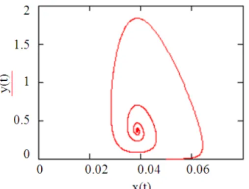
Fig. 3: Existence of limit cycles for r = 1, k = 0.5,m = 2, α = 0.51, b = 1,q₁ = 0.001,E₁ = 1,D = 1,s = 10,q₂ = 0.02, E₂ = 0.5, x(0) = 0.01, y(0) = 1, T1 = 100, p = 2

Fig. 4: Existence of limit cycles for choosing r = 1, k = 0.5, m = 2, α = 0.51, b = 1, q₁ = 0.001,E₁ = 1,D = 1,s = 10,q₂ = 0.02, E₂ = 0.5, x(0) = 0.01, y(0) = 0.5, T1 = 100, p = 2

Remark 5.2: we may note that our examples and

graphs are different from those exist in (Kar and Matsuda, 2007; Moghadas and Corbett, 2008).

COUCLUSION

In this article we discuss the existence and stability of equilibrium points using Routh-Hurwitz approach. Theorem1 shows that all solutions of the model are positive and bounded. We give sufficient condition guarantees that the model has at least one limit cycle in the first quadrant of the xy plane. We give sufficient condition guarantees that the model has at least one limit cycle in the first quadrant of the xy plane. We give sufficient condition guarantees that the model has at least one limit cycle in the first quadrant of the xy plane if:

1 1

x * g '(x*) g(x*)+ −y * p '(x*) _ q E <0

Using Bendixon Dulac Theorem we discuss the case for which the predator-prey model (1) has no periodic solution. Using Kuang and Freedman technique we give sufficient condition for the uniqueness of limit cycles of (1). Numerical examples for some special cases of g(x) are given to justify the results with graphs showing the existence of limit cycles.

REFERENCES

Attili, B.S. and S.F. Mallak, 2006. Existence of limit cycles in a predator-prey system with a functional response of the form Arctan(ax). Commun. Math. Anal., 1: 33-40.

Attili, B.S., 2001. Existence of limit cycles in a predator-prey system with a functional response. Int. J. Math. Sci., 27: 377-385. DOI: 10.1155/S016117120100655X

Freedman, H.I. and J.W.H. So, 1985. Global stability and persistence of simple food chains, Math. Biosci., 76: 69-86. DOI: 10.1016/0025-5564(85)90047-1

Hasik, K., 2000. Uniqueness of limit cycle in the predator–prey system with symmetric prey isocline. Math. Biosci., 164: 203-215. DOI: 10.1016/S0025-5564(00)00007-9

Hesaaraki, M. and S.M. Moghadas, 2001. Existence of limit cycles for predator–prey systems with a class of functional responses. Ecol. Model., 142: 1-9. DOI: 10.1016/S0304-3800(00)00442-7

Kar, T.K. and H. Matsuda, 2007. Global dynamics and controllability of a harvested prey–predator system with Holling type III functional response. J. Nonlinear Anal. Hybrid Syst., 1: 59-67. DOI: 10.1016/j.nahs.2006.03.002

Kelley, W.G. and A.C. Peterson, 2003. The Theory of Differential Equations: Classical and Qualitative. 1st Edn., Prentice Hall, New Jersey, ISBN-10: 0131020269, pp: 432.

Kuang, Y. and H.I. Freedman, 1988. Uniqueness of limit cycles in Gause-type models of predator-prey systems. Math. Biosci., 88: 67-84. DOI: 10.1016/0025-5564(88)90049-1

Moghadas, S.M. and B.D. Corbett, 2008. Limit cycles in a generalized Gause-type predator–prey model, J. Chaos Solitons Fractals, 37: 1343-1355. DOI: 10.1016/j.chaos.2006.10.017

Moghadas, S.M. and M.E. Alexander, 2005. Dynamics of a generalized Gause-type predator–prey model with a seasonal functional response. J. Chaos Solitons Fractals, 23: 55-65. DOI: 10.1016/j.chaos.2004.04.030

Moghadas, S.M. and M.E. Alexander, 2006. Bifurcation and numerical analysis of a generalized Gause-type predator-prey model. J. Dynamics Continuous, Discrete Impulsive Syst. Series B, 13: 533-554.

Pimply, G.H., 1974. Periodic solutions of third order predator-prey equations simulating an immune response. Arch. Rational Mech. Anal., 55: 91-123. DOI: 10.1007/BF00249934

Ruan, S. and D. Xiao, 2001. Global analysis in a predator-prey system with nonmonotonic functional response, SIAM J. Appl. Math., 61: 1445-1472.

Saha, T. and M. Bandyopadhyay, 2005. Dynamical analysis of a plant-herbivore model bifurcation and global stability. J. Applied Math. Comput., 19: 327 -344. DOI: 10.1007/BF02935808

Sesay, M.S., B.M. Abdulhamid and S.O. Aliyu, 2010. On the two-parameter bifurcation in a predator-prey system of Ivlev type. Pacific J. Sci. Technol., 11: 266-271.

Sugie, J., R. Kohno and R. Miyazaki, 1997. On a predator-prey system of Holling type. J. Proc. Am. Soc., 125: 2041-2050. DOI: 10.1090/S0002-9939-97-03901-4

Tao, Y., X. Wang and X. Song, 2011. Effect of prey refuge on a harvested predator–prey model with generalized functional response. Commun. Nonlinear Sci. Numer. Simulat., 16: 1052-1059. DOI: 10.1016/j.cnsns.2010.05.026