www.atmos-chem-phys.net/11/1177/2011/ doi:10.5194/acp-11-1177-2011
© Author(s) 2011. CC Attribution 3.0 License.
Chemistry
and Physics
Solar irradiance at the earth’s surface: long-term behavior observed
at the South Pole
J. E. Frederick and A. L. Hodge
Department of the Geophysical Sciences, University of Chicago, Chicago, Illinois, USA Received: 24 September 2010 – Published in Atmos. Chem. Phys. Discuss.: 3 November 2010 Revised: 20 January 2011 – Accepted: 3 February 2011 – Published: 11 February 2011
Abstract. This research examines a 17-year database of UV-A (320–400 nm) and visible (400–600 nm) solar irradi-ance obtained by a scanning spectroradiometer located at the South Pole. The goal is to define the variability in solar ir-radiance reaching the polar surface, with emphasis on the influence of cloudiness and on identifying systematic trends and possible links to the solar cycle. To eliminate changes associated with the varying solar elevation, the analysis fo-cuses on data averaged over 30–35 day periods centered on each year’s austral summer solstice. The long-term aver-age effect of South Polar clouds is a small attenuation, with the mean measured irradiances being about 5–6% less than the clear-sky values, although at any specific time clouds may reduce or enhance the signal that reaches the sensor. The instantaneous fractional attenuation or enhancement is wavelength dependent, where the percent deviation from the clear-sky irradiance at 400–600 nm is typically 2.5 times that at 320–340 nm. When averaged over the period near each year’s summer solstice, significant correlations appear be-tween irradiances at all wavelengths and the solar cycle as measured by the 10.7 cm solar radio flux. An approximate 1.8±1.0% decrease in ground-level irradiance occurs from solar maximum to solar minimum for the wavelength band 320–400 nm. The corresponding decrease for 400–600 nm is 2.4±1.9%. The best-estimate declines appear too large to originate in the sun. If the correlations have a geophysical origin, they suggest a small variation in atmospheric attenua-tion with the solar cycle over the period of observaattenua-tion, with the greatest attenuation occurring at solar minimum.
Correspondence to:J. E. Frederick ([email protected])
1 Introduction
Solar radiation reaching the Earth’s surface varies over a range of spatial and temporal scales. These variations include erratic short-term fluctuations associated with local cloudi-ness, longer-term changes in atmospheric attenuation on re-gional or global scales (Wild, 2009), and changes in the ex-traterrestrial irradiance over the 11-year solar cycle (Willson, 1997; Fr¨ohlich, 2009) and the very long time scale of stellar evolution (Gough, 1981).
The depletion of springtime stratospheric ozone amounts over Antarctica motivated concerns over changes in biolog-ically relevant solar ultraviolet radiation during the 1980’s and 1990’s (Weiler and Penhale, 1994). Since that time long-term measurements have been conducted at both high and middle latitudes (e.g. Liao and Frederick, 2005; Hicke et al., 2008) where the emphasis was on the influence of changing ozone amounts. Although ultraviolet radiation is clearly a significant environmental parameter, enhanced interest in the Earth’s climate system as a whole has focused attention on a wider range of the sun’s emission. It is increasingly im-portant to characterize all portions of the extraterrestrial and surface solar irradiance so as to define variations over all time scales. Issues of relevance here include variations inherent in the sun, the role of cloudiness, and any factor that influences the transmission of the Earth’s atmosphere (Wild, 2009).
2 The dataset
This work considers measured irradiances integrated over the wavelength bands 320–340 nm, 340–360 nm, 360–400 nm, and 400–600 nm expressed in W m−2. The time period of
interest extends from December 1992 to January 2009. All measured irradiances are accompanied by calculated values appropriate to clear skies using column ozone amounts de-rived from the spectroradiometer data (Bernhard et al., 2003). Details of the calculations appear in Bernhard et al. (2004).
The instrument is part of the National Science Founda-tion’s Ultraviolet Radiation Monitoring Network, operated by Biospherical Instruments, Inc. The sensor is a scanning spectroradiometer consisting of a quartz window and dif-fuser plate at the optical entrance, a double monochromator, a photomultiplier as the detector, and associated electronics. The spectral resolution is approximately 1.0 nm. On-site per-sonnel perform calibrations using standard lamps on a pe-riodic basis (Bernhard et al., 2008). Special attention has focused on developing an uncertainty budget for the mea-surements, including corrections for an imperfect cosine re-sponse (Bernhard et al., 2004). The measurements represent the sum of direct and diffuse downward solar spectral irradi-ances from 280 nm to 600 nm in wavelength. Further details of the instrument and the data processing appear in Booth et al. (1994) and Bernhard et al. (2004).
The solar irradiance incident on a horizontal surface is a sensitive function of solar zenith angle (SZA), and any anal-ysis of variability in irradiance must control for changes in SZA. The South Pole is distinguished by the fact that the SZA is essentially constant during an extended period around the December solstice of each year. To utilize this fact, we use only irradiance data collected when the SZA was within 1◦of its annual minimum value. This corresponds to dates from 7 December through 8 January, defined here as a “sol-stice period” and labeled by the calendar year which contains December. For example, the 2003 solstice period extends from 7 December 2003 to 8 January 2004 during which time the SZA always lies in the range 66.56 to 67.56◦. The en-tire dataset consists of 17 consecutive solstice periods, 1992 through 2008, with a total of 37 173 irradiance measure-ments in each wavelength band. Although data exist for the 1991 solstice period, the observations are contaminated by excess atmospheric aerosols associated with the eruption of the Pinatubo volcano in April of that year. We therefore elim-inated this particular solstice period from consideration.
Figure 1a–b presents the entire dataset of measured and computed clear-sky irradiances, respectively, for the wave-length band 320–340 nm, where the horizontal axis is the year which labels each solstice period. Figure 2a–b is analo-gous for the spectral region 400–600 nm. Several features in Figs. 1 and 2 merit comment. First, the clear-sky computed irradiances (Figs. 1b and 2b) show a relatively small variation within a single solstice period. This arises from the one de-gree spread in SZA and from weak attenuation by ozone in
Fig. 1.The irradiance dataset for the wavelength band 320–340 nm covering 17 solstice periods, 1992–2008:(a)Measured values.(b) Computed clear-sky values.
the wavelength bands 320–340 nm and 400–600 nm, while absorption by ozone is negligible between 340 and 400 nm (Molina and Molina, 1986; World Meteorological Organiza-tion, 1985). Column ozone amounts in early December are particularly variable owing to interannual differences in the dissipation of each year’s springtime ozone reduction. Next, the variability in measured irradiance (Figs. 1a and 2a) dur-ing any one solstice period is substantially greater than in the corresponding clear-sky values. This is the expected result of varying cloudiness. Furthermore, measured irradiances in excess of the clear-sky values occur in both spectral bands, indicating that cloudiness can both decrease and increase ground-level irradiance. Finally, the percentage variability in irradiance at 400–600 nm is substantially greater than at 320–340 nm.
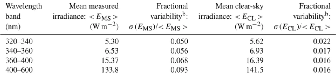
Table 1 presents some statistical properties of the dataset for all four wavelength bands, where the symbolsEMS and ECLrefer to the measured and clear-sky irradiances,
respec-tively. Note in particular the fractional variability, defined as the ratio of the standard deviation to the mean irradiance,
σ(EMS)/ < EMS>andσ(ECL)/ < ECL>, based on all data
points for each wavelength band. For the clear-sky calcula-tionsσ(ECL)/ < ECL>is greatest at the shortest wavelength
Table 1.Statistical characteristics of the irradiance dataseta.
Wavelength Mean measured Fractional Mean clear-sky Fractional band irradiance:< EMS> variabilityb: irradiance:< ECL> variabilityb: (nm) (W m−2) σ (EMS)/< EMS> (W m−2) σ (ECL)/< ECL>
320–340 5.30 0.050 5.62 0.022
340–360 6.53 0.056 6.93 0.017
360–400 15.37 0.068 16.39 0.016
400–600 133.8 0.093 141.5 0.016
aBased on 37 173 data points at each wavelength. bRatio of standard deviation to the mean irradiance.
Fig. 2.The irradiance dataset for the wavelength band 400–600 nm covering 17 solstice periods, 1992–2008:(a)Measured values.(b) Computed clear-sky values.
the small variation in SZA. The measured irradiances show a very different pattern. Here the fractional variability rep-resented byσ(EMS)/ < EMS>increases systematically with
increasing wavelength, reaching almost six times the clear-sky value in the 400–600 nm wavelength band.
To characterize the influence of cloudiness on surface irra-diance it is useful to define a quantity that is independent of both the ozone amount and the SZA. The ratio of measured to clear-sky irradiance serves this purpose:
R(λ)=EMS(λ,θ )/ECL(λ,θ,) (1)
whereλlabels a wavelength band, and the calculation in the denominator uses the SZAθappropriate to the measurement and a column ozone value derived from the spectrora-diometer data.
In an ideal circumstance, the value of the irradiance ratio would depend only on the influence of clouds and any other form of atmospheric opacity that affects the measurements but that is not included in the clear-sky calculations. In prac-tice, however, several factors related to instrument perfor-mance can influence the measured irradiance. A detailed un-certainty budget for irradiance at three wavelengths, 310, 400 and 600 nm, appears in Bernhard et al. (2004). A substan-tial source of uncertainty, 2.1% (600 nm) to 2.7% (310 nm), centers on absolute calibration and stability. An additional uncertainty associated with the cosine response of the dif-fuser plate depends on details of the prevailing clouds, and for SZA = 70◦this can be as large as 1.0% (310 nm) to 2.8% (600 nm) when the sky condition is unknown. The geophys-ical variations of interest in Section 4 of this paper can be of the same order as the above uncertainties. Fortunately, er-rors that are independent of time do not impact the primary conclusions. However, uncorrected drifts or discontinuities could be misconstrued as a linear trend over time, and the statistical analyses in Sect. 4 must acknowledge this possi-bility.
Fig. 3. Irradiance ratios for the solstice period December 2001 to January 2002, a relatively clear period:(a)320–340 nm wavelength band. (b)400–600 nm wavelength band. Day number 1 is 7 De-cember 2001.
irradiance ratios deviate from 1.0, the deviation for the 400– 600 nm band is always greater, either positive or negative, than that at 320–340 nm.
The box plots for 320–340 nm and 400–600 nm in Fig. 5 further illustrate the wavelength dependence associated with cloudiness. These summarize the statistical properties of the entire dataset where the upper and lower boxes, respectively, identify the second and third quartiles of the measurements, and the horizontal line separating these boxes is the median. The vertical line segments with error bars similarly define the first and fourth quartiles, while the x-symbols denote out-liers. The small squares at 0.94–0.95 for each wavelength are the mean irradiance ratios. Although these are virtually the same at both wavelengths shown, as well as for the 340– 360 nm and 360–400 nm bands (not shown), the variability increases substantially with wavelength. Furthermore, irra-diance ratios in excess of 1.0 are far more common in the 400–600 nm band than at 320–340 nm.
To further define the spectral character of the attenua-tions and enhancements provided by clouds, Fig. 6 plots the irradiance ratios at 320–340 nm versus those at 400– 600 nm for the entire database. The line with a slope of 1.0 illustrates the case of no wavelength dependence and obviously deviates from the measurements which form an envelope of much smaller slope. A least squares fit
Fig. 4. Irradiance ratios for the solstice period December 2007 to January 2008, a relatively cloudy period: (a)320–340 nm wave-length band.(b)400–600 nm wavelength band. Day number 1 is 7 December 2007.
to the individual points has the form R(320–340 nm) = (0.565±0.003) + (0.402±0.003)R(400–600 nm) where the error bars are two standard errors, and the regression ex-plains 67.6% of the variance. This shows quantitatively that the 320–340 nm signal has much less variation in response to changing cloudiness than does that for 400–600 nm.
Figure 7a–b, for 320–340 nm and 400–600 nm, defines the multi-year behavior of the irradiance ratios as well as an index of the variability within each solstice period. The dots depict the mean irradiance ratio for each solstice period, while the error bars are plus and minus one standard devi-ation. The different degree of variability in the two wave-length bands is apparent from the widths of the error bars.
One approach to addressing this is to assume that the “true” irradiance ratios are independent of wavelength, R(320–340 nm) = R(400–600 nm), and that the wavelength dependence derived from Fig. 6 is an artifact of uncorrected errors. How large must these errors be in order to produce the regression equation derived above?
IfR(400–600 nm)= 1.2, corresponding to a partly cloudy sky with the solar disk not obscured, then the regression-based value of R(320–340 nm) is 12.7% smaller than the “true” value (1.0474 versus 1.2). If R(400–600 nm)= 0.6, corresponding to an obscured solar disk and a sky likely 100% cloud covered, then the measured value of R(320– 340 nm)is 31.9% larger than the “true” value (0.7912 ver-sus 0.6). The result for the case ofR(400–600 nm)= 0.6 is especially important since the diffuse irradiance should be nearly isotropic over the hemisphere here, minimizing the uncertainty in the cosine correction. Although the above ar-gument is not definitive, these differences seem unreason-ably large to arise entirely from uncorrected cosine errors. In any event, Fig. 11, to be discussed later, shows that a purely model-based calculation produces a wavelength dependence remarkably close to that deduced from the measurements. This approach provides a convincing argument that the em-pirical results are valid.
Several features of the dataset require an explanation grounded in a theoretical understanding of the processes at work. These are (1) irradiances larger than the clear-sky val-ues are frequent occurrences, and (2) the variability in irradi-ance associated with cloudiness is greater in the visible than in the UV-A. The following section addresses these issues based on physical reasoning combined with a set of radiative transfer calculations that incorporate a simplified treatment of fractional cloudiness. The final topic of the paper involves interannual variability in cloudiness. The goal here is to de-termine whether the variations shown in Fig. 7 are seemingly random or whether there are systematic trends or possible links to solar activity.
3 Irradiances under partly cloudy skies: a theoretical analysis
Figure 6 shows that irradiances in excess of the clear sky value are common, particularly at 400–600 nm. A series of one-dimensional radiative transfer calculations based on the simplified cloud cover formulation first presented by Fred-erick and Erlick (1995) provides an explanation for this be-havior as well as for the wavelength dependence that appears when clouds are present. A number of previous studies have examined the wavelength dependent attenuation provided by clouds from both the empirical and theoretical standpoints (Seckmeyer et al., 1996; Frederick and Erlick, 1997; Kylling et al., 1997; Lindfors and Arola, 2008). The present work fo-cuses specifically on effects associated with fractional cloud cover as opposed to a uniform cloud layer.
Fig. 5. Box plots of all irradiance ratios for the 320–340 nm and 400–600 nm wavelength bands. The upper and lower boxes, respec-tively, for each wavelength define the second and third quartiles of the measurements. The upper and lower vertical lines, respectively, define the first and fourth quartiles. Small squares in the third quar-tile for each wavelength represent means, and the x-symbols are outliers.
Fig. 6. Dark circles denote measured irradiance ratios for 320– 340 nm plotted against those for 400–600 nm, showing the wave-length dependence in the attenuation or enhancement in solar irra-diance associated with South Polar clouds. The straight line and squares indicate a hypothetical case of no wavelength dependence.
Fig. 7. Statistical summary of irradiance ratios for each solstice period: dots are mean irradiance ratios. Error bars are plus and minus one standard deviation and indicate the variability associated with cloudiness.(a)320–340 nm wavelength band.(b)400–600 nm wavelength band.
1970). The problem is then cast in the form of two radiative transfer equations, one for downward diffuse and the other for upward diffuse irradiance, where the direct irradiance is obtained via Beer’s Law. The calculation treats absorption by ozone using a specified vertical profile, Rayleigh scattering based on a polar density profile and reflection from a lower boundary.
The handling of fractional cloudiness is a unique aspect of the calculation. Note that any attempt to incorporate the effects of fractional cloudiness into a one-dimensional calcu-lation must rest on major assumptions since the true radia-tive transfer problem is inherently three-dimensional. The model treats a cloud as a diffusing surface placed at a spec-ified altitude, where a fractionfcof the upper hemisphere is
covered by clouds of albedoAc. For ease of discussion we
adopt the same cloud albedo for both direct and diffuse in-cident radiation, although this is not true in general. The following quantities are computed as part of the solution to the radiative transfer equation:Ea(dn) is the downward
dif-fuse irradiance incident on the cloud top from above,Ea(dir)
is the downward direct irradiance incident on the cloud top from above andEb(up) is the upward diffuse irradiance
inci-dent on the cloud base from below. Given these, the
cloud-treatment computes the downward diffuse irradiance at the cloud base, labeled asEb(dn), and the upward diffuse
irradi-ance at the cloud top, labeled asEa(up).
When no absorption occurs inside the cloud, conservation of energy requires the following conditions to be true:
Eb(dn)=fc(1−Ac)[Ea(dir)+Ea(dn)] +fcAc[Eb(up)]
+(1−fc)[Ea(dn)] (2)
Ea(up)=fc(1−Ac)[Eb(up)] +fcAc[Ea(dir)+Ea(dn)]
+(1−fc)[Eb(up)] (3)
Eb(dir)=(1−fc)[Ea(dir)] (4)
The expressions for the diffuse irradiances, Eb(dn) and
Ea(up), require no further modification. However, the
ex-pression for the direct irradiance that comes though the clear fraction of the sky is problematic. Averaged over a substan-tial horizontal area, the above three equations must be true to ensure energy conservation. But at any specific location at the ground, the solar disk is likely to be totally visible or totally obscured by clouds. It is as iffcin Eq. (4) takes on
only the valuesfc=0 orfc=1 regardless of the actual value
of fractional cloudiness used in the calculation of diffuse ir-radiances.
The calculation allows the solar disk to be either entirely visible, which leads to irradiances in excess of the clear-sky value when clouds are present, or entirely obscured by clouds, which leads to irradiances less than the clear sky value. The computed diffuse irradiance can be interpreted as an average over the horizontal area to which the frac-tional cloud cover refers, while the computed direct irradi-ance refers to the specific location of the sensor.
Over the South Pole, the surface albedo is horizontally homogeneous, which is consistent with a one-dimensional calculation. Also, the clouds, particularly when fractional cloudiness prevails, are likely to be thin, so that compli-cations associated with the sides of clouds are minimized. Still, the calculation seeks to capture the physics of a three-dimensional situation in a one-three-dimensional model. While the calculations illustrate the mechanisms at work, one should not use the radiative transfer model to infer properties of the clouds from the measurements
To see how irradiances larger than the clear-sky values oc-cur, consider a sky that is partly covered by clouds, withfc
andAcas defined above. Assume that, as viewed from the
lo-cation of a ground-based sensor, the solar disk is in the clear portion of the sky. The irradiance that strikes the sensor con-sists of a direct component, which is identical to what would exist under a clear sky, and a diffuse component that repre-sents contributions from both the clear and cloudy portions of the sky.
fraction 1−Acof the incident diffuse radiation is transmitted
through the cloud. ForAc>0 this mechanism always acts
to decrease the irradiance that ultimately reaches a ground-based sensor. Similarly, the direct component of solar irra-diance incident on the cloud tops is partially reflected back upward and partially transmitted through the cloud, where a portion emerges as downward diffuse radiation. From this description, the direct solar beam influences the total irra-diance received by the sensor in two ways. First, since the sun lies in the clear portion of the sky, the entire direct so-lar beam reaches the sensor. Second, a fraction of the direct solar irradiance is transmitted through the clouds, emerges as diffuse radiation, and some of this reaches the sensor. In some circumstances, this second contribution can increase the irradiance over what would exist under clear skies.
The backscattering of diffuse radiation incident on the cloud tops represents a loss of irradiance from the ground. But the transmission of direct radiation through the cloud, and its conversion to diffuse radiation in the process, rep-resents a gain. If the gain in diffuse irradiance traceable to downward scattering of the direct solar beam in the clouds exceeds the loss from backscattering of diffuse radiation in-cident on the cloud tops, then the total irradiance measured at the ground will be greater than the value for clear skies.
Based on the above processes, measured irradiances in ex-cess of the clear-sky value require the sky to be partly cloudy, with the solar disk in the clear portion of the sky as viewed from the sensor. This is a necessary, but not a sufficient, con-dition. As the ratio of direct to diffuse irradiance incident on the cloud top increases, the probability of an enhancement in ground-level irradiance over the clear-sky values also in-creases. This implies that irradiance ratios greater than 1.0 should be more common at the longer wavelengths observed. Figure 5 shows this to be the case. Should the solar disk be-come obscured by cloudiness as seen from the sensor, the direct beam is lost, and the irradiance will drop to levels less than those for a clear sky.
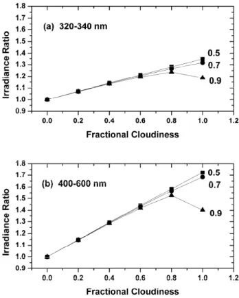
Figure 8a–b, for the wavelength bands 320–340 nm and 400–600 nm, illustrates the processes at work. Each panel presents the irradiance ratio computed as a function of frac-tional cloudinessfc, where the solar disk is in the clear
por-tion of the sky. The ground albedo is set toAG= 0 in both
cases so as to highlight the mechanism discussed above. The casefc=1 corresponds to complete cloud cover except for a
small break that coincides with the line of sight to the sun as viewed from the sensor. Each panel includes results for three cloud albedos,Ac=0.5, 0.7and 0.9.
A large ratio of direct to diffuse irradiance at the cloud top promotes surface irradiances greater than the clear-sky value, and this ratio is wavelength dependent as a simple re-sult of Rayleigh scattering. This wavelength dependent effect is evident in comparing Fig. 8a and b, where irradiance ratios larger than 1.0 arise most readily in the 400–600 nm wave-length band. Figure 8a for 320–340 nm shows that when the cloud albedo isAc=0.5 a small enhancement exists for all
Fig. 8.Computed irradiance ratios as functions of fractional cloudi-ness for cloud albedos ofAc=0.5, 0.7and 0.9. The solar disk is not
obscured by clouds, and the ground albedo isAG=0.0. (a)320–
340 nm wavelength band.(b)400–600 nm wavelength band.
values of fractional cloudiness. WhenAc=0.7 or 0.9
trans-mission through the cloud is restricted, and the surface irra-diance is less than the clear-sky result. In the 400–600 nm band (Fig. 8b) the diffuse irradiance incident on the cloud top is relatively small compared to the direct component. The mechanisms discussed above now lead to an increase in ground-level irradiance with fractional cloudiness for cloud albedos of 0.5 and 0.7, where all values exceed the clear-sky irradiance. When the cloud albedo reaches 0.9, the radiation that emerges downward from the cloud base is always less than would exist under clear skies, and the effect is to reduce the irradiance received at the ground.
A comparison of Fig. 8a and b for a cloud albedo ofAc=
0.7 reveals an unexpected and interesting result. As frac-tional cloud cover increases, the ground-level irradiance for 400–600 nm increases, while that at 320–340 nm decreases. This demonstrates that even the sign of the change in irra-diance for a specified change in cloudiness can depend on wavelength and details of the prevailing sky cover.
The above arguments considered only the direct and dif-fuse radiation incident on cloud tops. Another important mechanism for enhancing surface irradiance centers on the albedo AG of the lower boundary. When AG is large, as
Fig. 9.Computed irradiance ratios as functions of fractional cloudi-ness for cloud albedos ofAc=0.5, 0.7and 0.9. The solar disk is not
obscured by clouds, and the ground albedo isAG=0.98.(a)320–
340 nm wavelength band.(b)400–600 nm wavelength band.
the ground and cloud enhance the irradiance that reaches a sensor. Under conditions of fractional cloud cover, the solar disk may be visible as viewed from the ground-based sen-sor; however, the clouds will hide the disk as seen from other nearby locations. If fractional cloudinessfcis small, a
rela-tively large direct irradiance reaches the ground when aver-aged over the area of interest, and multiple reflections occur between the ground and cloud base. However, the small frac-tional cloud cover limits the magnitude of the resulting irra-diance enhancement. As fc increases, a larger cloud-base
area backscatters upwelling radiation, but the increased area-averaged blockage of the solar disk acts to limit the amount of energy that penetrates beneath the cloud and is available for this reflection. The result is that the irradiance observed by a sensor increases withfcup to some maximum,
depend-ing on the cloud albedo, and then can decline with further increases in fractional cloudiness.
Figure 9a–b is analogous to Fig. 8a–b except that the ground albedo is AG=0.98, typical of the Antarctic
sur-face (Grenfell et al., 1994). Even under clear skies this large albedo produces significantly enhanced irradiances rel-ative to the caseAG=0.0. For the wavelength band 400–
600 nm the increase is 8.2%, while at 320–340 nm the cor-responding number is 38.5%. The larger clear-sky
percent-age increase at the shorter wavelengths arises from stronger Rayleigh backscattering of radiation previously reflected up-ward at the lower boundary.
The irradiance ratios in Fig. 9a–b display the behavior ex-pected from the physical reasoning presented above. When fractional cloudiness exceeds 0.8 for the highest cloud albedo (Ac=0.9) the solar energy beneath the cloud is severely
limited and increases from multiple reflections between the ground and cloud base are inhibited. In this case, irradiance declines with further increases infc. Finally, Fig. 10a–b, for
the wavelength bands 320–340 nm and 400–600 nm, illus-trates the effect of the solar disk being obscured by clouds. The casefc= 0 here refers to a cloud-free sky except for a
small disk of albedoAc that coincides with the location of
the sun. The three curves in each panel depict irradiance ra-tios for cloud albedos ofAc=0.5, 0.7 and 0.9, respectively,
and the surface albedo isAG=0.98 in all cases. Note the
wavelength dependence in the attenuation, where the effect of clouds for 400–600 nm is usually exaggerated relative to that at 320–340 nm.
Figures 9 and 10 demonstrate that radiative transfer theory applied to partly-cloudy skies produces the wavelength-dependent attenuation and enhancement observed at the South Pole. Figure 11, based entirely on radiative transfer calculations, presentsR(320–340 nm)plotted againstR(400– 600 nm). The results are very similar to the analogous em-pirical plot in Fig. 6. A linear fit to the computed curve gives R(320–340 nm) = (0.589±0.011) + (0.430±0.010)R(400– 600 nm), where the slope is only 7% larger than the value derived from Fig. 6.
4 Long-term behavior of the irradiance ratios
This section considers relationships between the irradiance ratios and indices of interannual variability. The goal is to determine if the solar irradiance, as depicted in Fig. 7, con-tains systematic behavior over the time period of observation or if the year-to-year variation is random. Mean irradiance ratios for any solstice period characterize the net influence of clouds, and all other forms of variation not included in the clear-sky calculations, on solar irradiance at the ground. The analysis below considers two forms of long-term variability: (1) linear trends in time and (2) links to the solar cycle. The calendar year that contains December provides the measure of time, while we characterize the solar cycle by the mean 10.7 cm solar radio flux (F10.7)adjusted to 1.0 Astronomical
Unit for each solstice period (NOAA National Geophysical Data Center, 2010). Figure 12 presents this indicator of solar activity for the period studied. Note that the value ofF10.7
for the 2001 solstice period is unusually large.
Fig. 10. Computed irradiance ratios as functions of fractional cloudiness for cloud albedos ofAc=0.5, 0.7 and 0.9. The solar
disk is obscured by clouds, and the ground albedo isAG=0.98.(a)
320–340 nm wavelength band.(b)400–600 nm wavelength band.
Fig. 11.Computed irradiance ratios for 320–340 nm plotted against those for 400–600 nm, showing the wavelength dependence in the attenuation or enhancement in solar irradiance associated with clouds as produced by theory. Open circles define the case of no wavelength dependence. The solid line is a fit to radiative transfer calculations indicated by squares.
Fig. 12.Solar 10.7 cm radio flux in relative units: points are means of daily measured values for each 30–35 day solstice period.
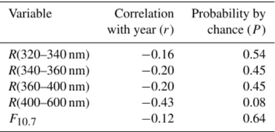
arise by chance. For future reference, the correlation be-tweenF10.7and year appears as well. Based on the standard
criterion ofP <0.05, the irradiance ratios and the 10.7 cm flux contain no significant linear trends over time, although some indication of a downward trend exists (P =0.08) in the 400–600 nm irradiance ratio. If we interpret the behavior as a linear change over time, it corresponds to a decrease of approximately 1.5±1.6% per decade, where the 95% confi-dence interval encompasses zero.
The hint of a downward trend in the visible band merits further attention. A systematic change in cloudiness would preferentially influence the 400–600 nm irradiance owing to the enhanced sensitivity of the signal at longer wavelengths. Furthermore, clouds over the South Pole induce erratic vari-ability into the irradiance (Figs. 3 and 4), so that a long-term trend in cloudiness should appear in the irradiance ra-tios and their standard deviations. Specifically, unusually cloudy solstice periods would exhibit both small mean irra-diance ratios and large standard deviations. However, sta-tistical analysis shows no significant trend in the standard deviation for 400–600 nm, the correlation with year being
r=0.31 with P=0.23. The small correlations found for the other wavelength bands have even greater probabilities of arising by chance. Based on the information available, there is no compelling evidence of a trend in cloudiness over the South Pole for the time period studied. Statistically insignifi-cant changes of the magnitude derived for 400–600 nm could arise by chance or from systematic errors in the dataset asso-ciated, for example, with replacement of instrument compo-nents.
based on all 17 solstice periods and on only 16 periods, with 2001 omitted. We regard the former case to be the primary result, but want to ensure that removal of one particular year does not alter the general conclusion. When all 17 years en-ter the calculation, significant positive correlations exist for each wavelength band, withP <0.01 in the ultraviolet and
P <0.05 in the visible. With 2001 omitted, significant corre-lations remain at the 5% level of confidence. The absence of temporal trends in the irradiance ratios and inF10.7(Table 2)
ensures that the results in Table 3 do not arise from an ac-cidental confounding of linear behavior over time with solar activity. The conclusion from Table 3 is that the measured irradiances reaching the South Polar surface included a com-ponent that varied in phase with the solar cycle over the time period studied. This result applies both to the ultraviolet and visible regions.
The significant correlations in Table 3 motivated applica-tion of a regression model with the form:
R(λ)=a0+a1[F10.7−< F10.7>]/100+ε (5)
where< F10.7>is the average 10.7 cm radio flux for the
en-tire period of observation, the coefficientsa0anda1are to be
determined, andεincludes the unexplained variance. When all 17 solstice periods enter the regression< F10.7>=115.3,
and when the 2001 period is omitted< F10.7>=108.1.
Ta-ble 4 lists the estimated coefficients (a0,a1), their standard
errors (α0,α1), and the percent of variance explained by the
model based on all 17 years. Table 5 presents analogous re-sults with data for 2001 removed. A 100 unit change inF10.7
leads to a best-estimate percentage change in irradiance ratio of 100a1/a0, which corresponds approximately to the
dif-ference between solar maximum and solar minimum. The 95% confidence interval spans the range 100(a1-2α1)/a0to
100(a1+2α1)/a0. Table 6 presents these percentage changes.
When data from all years enter the regressions, the esti-mated irradiances for solar minimum are about 1.8% and 2.4% smaller than those at solar maximum for the wave-lengths 320–400 nm (representing all three UV-A bands combined) and 400–600 nm respectively, with a larger error bar in the visible. The solar cycle remains, with a some-what altered magnitude, when the regressions omit the 2001 solstice period. Here the estimated decrease from solar max-imum to solar minmax-imum is about 1.5% for 320–400 nm and 3.5% for 400–600 nm, again with a larger error bar in the visible. We regard numbers based on all 17 solstice peri-ods as the best estimates, but the persistence of a solar cycle dependence when data for 2001 are omitted indicates the ro-bustness of the result. If these changes have a geophysical or solar origin, they must arise from (1) variations in the trans-mission of the South Polar atmosphere over the solar cycle during the time period studied, (2) variations in the extrater-restrial solar irradiance, which are implicit in the spectro-radiometer measurements but are not included in the clear-sky calculations, or (3) a combination of both mechanisms. Alternate interpretations are (1) an uncorrected error in the
Table 2. Correlation of mean irradiance ratios with year (based on 17 Solstice Periods, 1992 through 2008).
Variable Correlation Probability by with year (r) chance (P)
R(320–340 nm) −0.16 0.54
R(340–360 nm) −0.20 0.45
R(360–400 nm) −0.20 0.45
R(400–600 nm) −0.43 0.08
F10.7 −0.12 0.64
measurements has an accidental correlation with the solar cy-cle or (2) the correlation is real in the mathematical sense but does not does arise from a causal physical link.
The data of Harder et al. (2009) and Haigh et al. (2010) also indicate an unexpected increase in the visible irradi-ance over the declining phase of the solar cycle from 2004 to 2007. The sign of the South Polar visible surface variation deduced here disagrees with these extraterrestrial observa-tions. The regression based on 17 years of surface data pro-duces a decrease in 400–600 nm irradiance of 2.4% from so-lar maximum to soso-lar minimum, with an uncertainty range of 0.5–4.3%. These percentages correspond to a decline in en-ergy flux striking a horizontal surface at the ground of about 3.4 W m−2, with an uncertainty range of 0.7-6.1 W m−2for a SZA near 67 degrees. Except perhaps for the very low end of the error range, these numbers are unacceptably large to interpret as being extraterrestrial. Even if one ignores the problem with the phase of the variation relative to the data of Harder et al. (2009) and Haigh et al. (2010), only num-bers near the lower limit of the range are compatible with measured decreases in the Solar Constant of about 0.1%, or 1.3 W m−2, from solar maximum to solar minimum (e.g.
Ca-halan et al, 2010).
One potential geophysical mechanism for changes in at-mospheric transmission from one solstice season to the next involves cloudiness. The possibility that clouds are linked to solar activity has appeared in the literature, although the con-cept is controversial and conflicting results exist (Svensmark, 1998, 2007; Sloan and Wolfendale, 2008). As noted previ-ously, clouds over the South Pole vary erratically. Hence, one expects differences in cloudiness between solstice seasons to appear both as a change in the mean value ofR(λ)as well as in its standard deviation. If the correlations betweenR(λ)
andF10.7arise from rapidly varying cloudiness whose details
change from year-to-year over the solar cycle, then a corre-lation should also exist between the standard deviations and
F10.7. Table 7 presents these correlation coefficients. When
short-Table 3.Correlation of mean irradiance ratiosR(λ)with the 10.7 cm solar radio flux.
Variable Correlation Probability by Correlation Probability by withF10.7(r) chance (P ) withF10.7(r) chance (P ) (17 years) (17 years) (Omit 2001) (Omit 2001)
R(320–340 nm) 0.74 0.001 0.54 0.030
R(340–360 nm) 0.72 0.001 0.54 0.030
R(360–400 nm) 0.62 0.008 0.54 0.032
R(400–600 nm) 0.55 0.021 0.61 0.012
Table 4.Results from the regression model:
R(λ) =a0+a1[(F10.7−<F10.7>)/100]+ε(applied to all 17 Sol-stice Periods).
Wavelength a0 αa0 a1 α∗1 %Variance
band (nm) explained
320–340 0.944 0.00201 0.0190 0.00451 54.1
340–360 0.942 0.00174 0.0158 0.00391 52.3
360–400 0.938 0.00220 0.0151 0.00494 38.4
400–600 0.948 0.00399 0.0231 0.00896 30.6
∗α
i=standard error of coefficientai,i=1,2.
Table 5.Results from the regression model:
R(λ)=a0+a1[(F10.7−<F10.7>)/100]+ε(applied to 16 Solstice Periods, Omitting Data for 2001).
Wavelength a0 α∗0 a1 α∗1 %Variance
band (nm) explained
320–340 0.942 0.00203 0.0142 0.00587 29.4
340–360 0.940 0.00179 0.0125 0.00517 29.3
360–400 0.937 0.00234 0.0161 0.00677 28.8
400–600 0.947 0.00400 0.0333 0.0116 37.2
∗α
i= standard error of coefficientai,i=1,2.
term variability of South Polar clouds are not the origin of the correlations in Tables 4 and 5.
Variability in the extraterrestrial solar irradiance provides an obvious explanation for the correlations in Table 3, al-though the estimated magnitudes are not necessarily consis-tent with current understanding. The space-based spectral irradiance measurements of Harder et al. (2009) and Haigh et al. (2010) show changes between 2004 and 2007, during the declining phase of the solar cycle, that differ in magni-tude and, at some wavelengths, in sign from accepted un-derstanding (Lean, 2000; Lean et al. 1997). The data pre-sented by Haigh et al. (2010) contain decreases in the 320– 400 nm spectral irradiance whose magnitudes are strongly wavelength dependent and which are generally much larger than predicted by the model of Lean (2000). Based on Fig. 1 of Haigh et al. (2010), the decline is roughly 0.5 W m−2when
integrated over 320–400 nm. This is similar to the full so-lar cycle change inferred from the South Poso-lar 320–400 nm surface data, being 1.5–1.8% of the absolute irradiances in Table 1.
Rapidly varying clouds provide a readily detected attenu-ation of incoming radiattenu-ation, but this work showed that South Polar clouds are not obviously correlated with the solar cy-cle. However, other contributors to the polar atmospheric opacity are conceivable. For example, persistent layers of scatterers such as ice crystals, which are too thin to appear as a readily-seen cloud, could exert a weak influence on the irradiance ratios. Such thin scattering layers could exist over the South Pole, and the attenuation they provide might have varied systematically on the time scale of the 11-year solar cycle during the period of the irradiance measurements. This hypothesis, although speculative, could explain the observed variability in ground-level solar irradiance, including the fact that the best estimate of the percent variation in the visible is larger than that in the UV-A.
5 Conclusions
Clouds over the South Pole act both to attenuate and to en-hance solar irradiance observed by a ground-based sensor. Averaged over the entire observing period, the overall effect of South Polar clouds is a small attenuation, with the mean measured irradiance being about 5–6% less than the clear-sky value for wavelengths between 320 and 600 nm. The fractional attenuation or enhancement at any instant of time is wavelength dependent, where the percent deviation from the clear-sky irradiance at 400–600 nm is typically 2.5 times that in the near ultraviolet at 320–340 nm. The occurrence of irradiances in excess of the clear-sky values and the ob-served wavelength dependence are consistent with radiative transfer calculations for a high-albedo lower surface, frac-tional cloud cover with the cloud albedo being independent of wavelength, and Rayleigh scattering.
Table 6.Percentage change in irradiance ratio for a 100-Unit Change in 10.7 cm solar radio flux (based on the regression models).
Wavelength Best estimate % 95% Confidence Best estimate % 95% Confidence band (nm) change inR(λ) range change inR(λ) range (17 years) (17 years) (Omit 2001) (Omit 2001)
320–340 2.0 1.0–3.0 1.5 0.3–2.8
340–360 1.7 0.9–2.5 1.3 0.2–2.4
360–400 1.6 0.6–2.6 1.7 0.3–3.2
400–600 2.4 0.5–4.3 3.5 1.1–6.0
Table 7.Correlation of standard deviations of irradiance ratios (σ) with the 10.7 cm solar radio flux.
Variable Correlation Probability by Correlation Probability by withF10.7(r) Chance (P ) withF10.7(r) Chance (P ) (17 years) (17 years) (Omit 2001) (Omit 2001)
σ(320–340 nm) −0.16 0.55 −0.45 0.08
σ(340–360 nm) −0.18 0.49 −0.47 0.07
σ(360–400 nm) −0.13 0.61 −0.41 0.11
σ(400–600 nm) −0.17 0.52 −0.41 0.12
significant correlations exist between irradiance ratios at all wavelengths studied and the 10.7 cm solar radio flux, where the quantities are averaged over individual solstice periods. Regressions based on all 17 solstice periods indicate approx-imate 1.8% and 2.4% decreases in ground-level irradiance for the wavelength regions 320–400 nm and 400–600 nm, re-spectively, from solar maximum to solar minimum. The as-sociated uncertainty ranges are approximately 0.8–2.7% for the UV-A and 0.5%–4.3% for the visible.
Changes in extraterrestrial irradiance over the solar cycle surely contribute a portion of the variability deduced at the polar surface for the 320–400 nm region, although the mag-nitude of this contribution is uncertain. However, the inferred solar cycle dependence in the 400–600 nm visible band is too large to be of extraterrestrial origin unless one adopts values at the lowest end of the error range. Uncorrected instrument drifts and discontinuities can always introduce artifacts into a dataset. However, for this to explain the observed behavior, any such unknown problems must have a spurious correla-tion with the solar cycle. Given the small magnitude of the inferred changes, the uncertainties in the measurements and the limited duration of the dataset, a confirmation of the solar cycle effect based on independent data would be of value. Acknowledgements. Support for instrument operation and data processing was provided by the National Science Foundation under prime award number OPP-0000373 granted to Biospherical Instruments, Inc. via subcontracts from Raytheon Polar Ser-vices Company. The authors thank Guoyong Wen for valuable discussions concerning the extraterrestrial solar irradiance and Germar Bernhard for a thorough and critical reading of the original manuscript.
Edited by: B. Mayer
References
Bernhard, G. C., Booth, C. R., and McPeters, R. D.: Cal-culation of total column ozone from global UV spectra at high latitudes, J. Geophys. Res.-Oc. Atm., 108(D17), 4532, doi:10.1029/2003JD003450, 2003.
Bernhard, G., Booth, C. R., and Ehramjian, J. C.: Version 2 data of the National Science Foundation’s ultraviolet radiation mon-itoring network: South Pole, J. Geophys. Res.-Oc. Atm., 109, D21207, doi:10.1029/2004JD004937, 2004.
Bernhard, G., McKenzie, R. L., Kotkamp, M., Wood, S., Booth, C. R., Ehramjian, J. C., Johnston, P., and Nichol, S. E.: Comparison of ultraviolet spectroradiometers in Antarctica, J. Geophys. Res.-Oc. Atm., 113, D14310, doi:10.1029/2007JD009489, 2008. Booth, C. R., Lucas, T. B., Morrow, J. H., Weiler, C. S., and
Pen-hale, P. A.: The United States National Science Foundation’s polar network for monitoring ultraviolet radiation, Ultraviolet Radiation in Antarctica: Measurements and Biological Effects, Antarc. Res. Ser., 62, edited by: Weiler, C. S., and Penhale, P. A., American Geophysical Union, Washington, DC, 17–37, 1994. Cahalan, R. F., Wen, G., Harder, J. W., and Pilewskie, P.:
Tempera-ture responses to spectral solar variability on decadal time scales, Geophys. Res. Lett., 37, L07705, doi:10.1029/2009GL041898, 2010.
Frederick, J. E. and Erlick, C.: Trends and interannual variability in erythemal irradiance, 1978–1993, Photochem. Photobiol., 62, 476–484, 1995.
mech-anisms, J. Atmos. Sci., 54, 2813–2819, 1997.
Fr¨ohlich, C.: Evidence of a long-term trend in total solar irra-diance, Astron. Astrophys., 501, L27–30, doi:10.1051/0004-6361/200912318, 2009.
Gough, D. O.: Solar interior structure and luminosity variations, Solar Phys., 74, 21–34, 1981.
Grenfell, T. C., Warren, S. G., and Mullen, P. C.: Reflection of solar radiation by the Antarctic snow surface at ultraviolet, visible, and near infrared wavelengths, J. Geophys. Res.-Oc. Atm., 99(D9), 18,669–18,684, 1994.
Haigh, J. D., Winning, A. R., Toumi, R., and Harder, J. W.: An influence of solar spectral variations on radiative forcing of cli-mate, Nature, 467, 696–699, doi:10.1038/nature09426, 2010. Harder, J. W., Fontenla, J. M., Pilewskie, P., and Richard,
E. K: Trends in solar spectral irradiance variability in the visible and infrared, Geophys. Res. Lett., 36, L07801, doi:10.1029/2008GL036797, 2009.
Hicke, J. A., Slusser, J., Lantz, K., and Pascual, F. G.: Trends and interabbual variability in surface UVB radiation over 8 to 11 years observed across the United States, J. Geophys. Res.-Oc. Atm., 113, D21302, doi:10.1029/2008JD009826, 2008. Kylling, A., Albold, A., and Seckmeyer, G.: Transmittance of a
cloud is wavelength dependent in the UV-range: physical inter-pretation, Geophys. Res. Lett., 24, 397–400, 1997.
Lean, J.: Evolution of the sun’s spectral irradiance since the Maun-der Minimum, Geophys. Res. Lett., 27, 2425–2428, 2000. Lean, J. L., Rottman, G. J., Kyle, H. L., Woods, T. N., Hickey, J. R.,
and Puga, L. C.: Detection and parameterization of variations in solar mid- and near-ultraviolet radiation (200–400 nm), J. Geo-phys. Res.-Oc. Atm., 102, 29,939–29,956, 1997.
Liao, Y. and Frederick, J. E.: The ultraviolet radiation environment of high southern latitudes: springtime behavior over a decadal timescale, Photochem. Photobiol., 81, 320–324, 2005.
Lindfors, A. and Arola, A.: On the wavelength-dependent attenua-tion of UV radiaattenua-tion by clouds, Geophys. Res. Lett., 35, L05806, doi:10.1029/2007GL032571, 2008.
Molina, L. T. and Molina, M. J.: Absolute absorption cross-sections of ozone in the 185 to 350 nm wavelength range, J. Geophys. Res.-Oc. Atm., 91, 14,501–14,508, 1986.
NOAA National Geophysical Data Center: http://www.ngdc.noaa. gov/, last access: 15 September 2010.
Seckmeyer, G., Erb, R., and Albold, A.: Transmission of a cloud is wavelength dependent in the UV-range, Geophys. Res. Lett., 23, 2753–2755, 1996.
Shettle, E. P. and Weinmann, J. A.: The transfer of solar irradiance through inhomogeneous turbid atmospheres evaluated by Ed-dington’s approximation, J. Atmos. Sci., 27, 1048–1055, 1970. Sloan, T. and Wolfendale, A. W.: Testing the proposed causal
link between cosmic rays and cloud cover, Environ. Res. Lett., 3, 024001, doi:10.1088/1748-9326/3/2/024001, 2008.
Svensmark, H.: Influence of cosmic rays on Earth’s climate, Phys. Rev. Lett., 81, 5027–5030, doi:10.1103/PhysRevLett.81.5027, 1998.
Svensmark, H.: Cosmoclimatology: a new theory emerges, Astron. Geophys., 48(1), 1.18–1.24, 2007.
Weiler, C. S. and Penhale, P. A. (Eds.): Ultraviolet Radiation in Antarctica: Measurements and Biological Effects, Antarc. Res. Ser., 62, American Geophysical Union, Washington, DC, 257 pp.,1994.
Wild, M.: Global dimming and brightening: A review, J. Geophys. Res.-Oc. Atm., 114, D00D16, doi:10.1029/2008JD011470, 2009.
Willson, R. C.: Total solar irradiance trend during solar cycles 21 and 22, Science, 277, 163–165, 1997.