www.adv-radio-sci.net/11/55/2013/ doi:10.5194/ars-11-55-2013
© Author(s) 2013. CC Attribution 3.0 License.
Radio Science
A fast three-dimensional deterministic ray tracing coverage
simulator for a 24 GHz anti-collision radar
H. Azodi, U. Siart, and T. F. Eibert
Lehrstuhl f¨ur Hochfrequenztechnik, Technische Universit¨at M¨unchen, Arcisstr. 21, 80333 Munich, Germany Correspondence to:H. Azodi ([email protected])
Abstract. A matrix-based approach for implementation of deterministic ray tracing is suggested and presented in this paper. The frequency-independent feature of the ray tracing in addition to the matrix-based implementation results in a reliable fast simulator for understanding the behavior of the electromagnetic fields in the vicinity of a collision avoidance radar. Results of this technique are in a good agreement with the results from method of moments integral equation solu-tions while the computasolu-tions are about 100 times faster.
1 Introduction
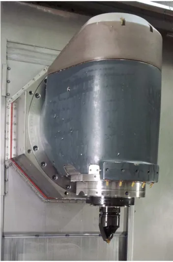
Computer numerical control (CNC) machines are a group of manually programmed modern machines for drilling, milling, laser or plasma cutting, etc. (Fig. 1). They are ranged within the expensive workshop machinery. Due to human er-rors in coding their controls, disastrous collisions between the tool of the machine and surrounding metallic objects can easily cause very expensive damage. It is, therefore, wise to detect possible collisions in advance and stop the machine. For this reason, we suggest to encircle the tool of CNC ma-chines with a number of radar modules to detect the possi-bility of harmful collisions and to stop the machine before collisions take place.
Figure 2 shows a mock-up of CNC tool and the radar mod-ules surrounding it. We propose to use the minimum of 3 modules with 120◦circular distance so that full coverage of
the surrounding space can be achieved. Thanks to the simple and symmetrical geometry any calculation or simulation for one module can be easily expanded for other modules in dif-ferent positions. The radiator of this module is a linear patch array antenna with 8 elements which operate in the ISM band around 24.125 GHz.
Due to frequent replacements of tool, object, etc., a CNC machine has a varying electromagnetic environment.
Conse-quently, the radar system requires to calibrate itself through-out the operational mode of the machine. On the other hand, the design should remain consistent and practically compat-ible with any CNC machine. These highly-demanding fea-tures require an accurate, fast, and reliable radar system. False alarms, not desirable though, are accepted but collision detection failure is not permitted at all.
From an electromagnetic point of view, this problem can be categorized in near-field antenna propagation modeling and channel estimation. Understanding the behavior of elec-tromagnetic (EM) waves in the vicinity of the tool plays the most important role in designing such a radar system. In the next section, we explain why ray tracing is a good candidate for simulating the fields and obtaining the channel model. In Sect. 3, the main idea of our fast deterministic ray trac-ing approach is explained and the results of this approach are presented in Sect. 4. Section 5 concludes this paper.
2 Electromagnetic modeling and solution technique
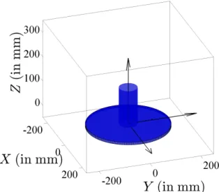
The mock-up, which contains the most important character-istics of the tool of the CNC machine, is modeled with two cylinders (Fig. 3). The antenna is located on the holder. As shown in Fig. 4, a single patch array antenna in an open PEC cavity is used. The electromagnetic modeling of the antenna itself and its local environment is decoupled from the propa-gation problem. The current electromagnetic model includes the most important aspects of the mock-up. A detailed model is simply created by adding more cylinders to the model. Therefore, we sticked to this simple model at this stage and for later stages we will add more complexities to the model. It is, indeed, possible due to flexibility of our simulation tech-nique which becomes evident to the readers in the rest.
Fig. 1.Tool of a CNC and its machinery
A typical FDTD code would need more than 10 lines/λ at
FCEN=24 GHz leads to 38 million mesh-cells for the struc-ture which takes several days of CPU time for every scenario on a quad-core computer with 12 GB of RAM. Moreover, 10 lines per wavelength is the minimum and for more accu-rate results an increase to 16 lines/λis recommended. Con-sequently, simulations at higher ISM bands such asFCEN= 60 GHz appear impractical.
The Method of Moments (MoM) – integral equation (IE) method is another potential solution candidate, particularly suitable due to the fully metallic surface of the geometry. The problem can therefore be discretized with about 5 million un-knowns at 24 GHz. This can be handled with the aforemen-tioned computer, although it is a big problem. Hence, the IE method is used as a standard method to compare and vali-date the results of the ray tracer as it is still a big problem for every-day optimization and design processes. For this pur-pose, an in-house IE-MoM code is used Eibert (2004).
The third candidate to solve this problem is ray tracing Ling et al. (1989). As mentioned in Sect. 1, this is a near-field problem. In contrary, ray tracing is a method where fields
Fig. 2.Initiative measurement mock-up designed and manufactured in our workshop and the Radar module on the surrounding area
are assumed to propagate in the far-field region. This is the estimation which should be taken into account in order to achieve the benefits of ray tracing method. This estimation can be improved by considering more geometrical details of the objects such as curvature, multiple reflections, etc. In our approach the problem of antenna simulation and field cal-culations are decoupled. The antenna far-field pattern is ob-tained using FDTD technique and it is inserted into the wave propagation ray tracing code. Once the ray paths to an ob-servation point is found, field calculation is a summation of the initial fields of antenna pattern multiplied by reflection or diffraction coefficients depends on path, free space loss and propagation phase shift.
Fig. 3. Electromagnetic modeling of the initiative mock-up.The problem is decoupled in modeling the geometrical scenario and an-tenna, separately.
This will bring the idea of deterministic ray tracing while we have a priori information by knowing the geometry of the problem.
Another problem arises in SBR when a ray closely passes the observation point. As an observation point is theoretically dimensionless, these rays are usually not included. Neverthe-less, it is seen that Flores et al. (1998); Noori et al. (2006) these missing rays might have an effect on the field of that point. Therefore, the idea of reception sphere is developed as a solution to this problem. In our deterministic ray tracing method, the observation point and all the other points remain dimensionless, i.e. ideal, and we are still able to calculate reaching paths to them accurately.
3 Fast matrix-based deterministic ray tracing
Deterministic ray tracing is suggested and developed in or-der to obtain the EM fields in the vicinity of the radar. This method enables us to have an overview of the coverage of the radiation strength and to estimate the channel response much faster than the aforementioned discretizing methods. As calculations are done usingsame-size matrices, a loop-less MATLAB® code will provides with the results in a few minutes on the used PC.
From a general perspective, the idea of matrix-based de-terministic ray tracing consists of two main parts. In the first part, the code calculates the required (mostly) geometrical matrices and the second part of the code is responsible for calculating the fields due the various rays and adding them together. These two parts are explained in Sects. 3.1 and 3.2, respectively.
Patch antenna and feeding line
Substrate
Antenna protection hole
Holder
Fig. 4. Modeling of antenna as a single patch in a box of PEC. The box is empty and the antenna is a single patch fed with mi-crostripline.
3.1 Pre-calculation and matrix formation
The entire observation space is discretized with equi-distant grids. For each grid in the observation space, there exists a unique element in every matrix. For example,X= [xmnp]is the X-coordinate of the grid in the position of(m, n, p)of the space. The same applies toYandZmatrices. Size of the ma-trices depends on the discretization fineness. The complexity of the problem increases with resolution as well but not with frequency.
Having these matrices, the rest of the pre-calculation phase is determining the geometrical matrices. For instance, the Eu-clidean distance to the origin:
R=hqx2
mnp+ymnp2 +z2mnp
i
(1) where all operations are element-wise. Equation (1) can be implemented in MATLAB® without using a loop. Any other required matrix can be calculated with the same principle.
The most important matrices in the pre-calculation phase areshadow (or illumination)matrices. Zero, 0, in a shadow (or one, 1, in an illumination) matrix means the corre-sponding observation point, Pmnp, is illuminated, counter-part means it is shadowed. Obviously, shadow matrices are ray dependent. These matrices contain the information of ray paths. So, in computation of them the Fermat’s principle is used. This means, for example, for the direct ray the direct path from the antenna to the observation point is considered. To calculate these matrices numerically, a geometry data matrix,BGEO, is created first. One, 1, inBGEOindicates that the corresponding point in the space is occupied with an ob-ject (or a part of an obob-ject). For empty space the matrix re-turns 0. Thus, the size of this matrix is the same as other ma-trices and if higher accuracy is required, finer discretization can be applied. The shadow matrix element for the observa-tion point(m, n, p)is, therefore,
smnp=
Pmnp
Z
Tmnp
BGEOdl≥1
ܺ
ܻ ܼ
TX
ͳ ʹ
͵
ͷ ܲሺݔǡ ݕǡ ݖሻ
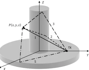
Fig. 5.5 rays contribute to find out the field in one point. They are identified with numbers on each path. As creeping ray and direct ray cannot reach an observation point together, in this schematic the chosen point is not illuminated by creeping ray.
whereTmnp is the position of the transmitter corresponding to the observation point atPmnp and the ray type. It should be noted again that depending on the ray type the transmitter position can be different from the antenna position. For in-stance in reflection from the cylinder, the transmitter is first the antenna but, later, when we need the path from the re-flection point to the observation point, it becomes a point on the cylinder. The reflection point is computed based on Fer-mat’s principle and is saved in the corresponding element of the “reflection point from the cylinder” matrix. The integral in Eq. (2) is over the connecting straight line between the pointsTmnpandPmnpand the integrand is the geometry data function of the space. By discretization,
smnp=
X
i
[bminipi] ≥1
!
(3)
where[bminipi]runs over the elements of geometry data ma-trix which fall in the connecting line of transmitter and ob-servation points. Calculating all smnp, the shadow matrix,
S= [smnp], is created.
The pre-calculation process is finished by calculating the geometrical matrices, shadow (or illumination) matrices and incident field matrices. Incident field matrices correspond to amplitude and phase of the fields which are just propagated in the direction of the ray path from the antenna. These fields are generated by interpolating the spherical coordinates of the direction and the far-field pattern.
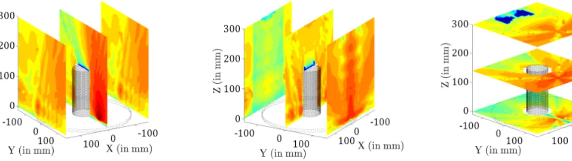
Fig. 6.Magnitude of E-field in surrounding space of the machine sliced every 45 degrees.
Contributions of 5 rays are summed up in our simula-tions. These rays are direct ray, reflected ray by the cylin-der, diffracted ray by the upper edge of cylincylin-der, creeping ray around the cylinder, and diffracted ray by the edge of the holder (Fig. 5).
3.2 Field calculation and summation
Except the direct path from the transmitted to the observa-tion point, the other paths are going through several points on the structure. The coordinates of these points in each ray type are calculated and stored in separate matrices. For ex-ample for the reflection from the cylinder, there is a point on the cylinder where the reflection occurs, obviously. The coordinates of this point are stored inXN,REF,YN,REF, and
ZN,REF, respectively. It should be noted again that the el-ements of matrices are in accordance with the observation point. This means thatXN,REF= [xmnp]has the first coor-dinate of the point NREF in accordance with the observa-tion pointPmnp.NREFcan be computed using the geomet-rical optics rule of reflection. Taking into account thatNREF is a point on the cylinder with, i.e. 0≤zmnp≤HCYL and
xmnp2 +ymnp2 =RCYL2 , whereHCYLandRCYLare height and radius of the cylinder, respectively, a quadratic equation is obtained which in principle has 4 roots. From them, only one is the desired root forPmnp. This root is real and belongs to the illuminated side of the cylinder. Thus, a direct solution Tignol (2004) to the equation will provide us with the desir-able result.
Fig. 7.Magnitude of E-field in surrounding space of the machine sliced w.r.t. X-, Y-, and Z-axes.
−200
0
200
−200
0
200
0
100
200
Y
(in mm)
X
(in mm)
Z
(i
n
mm)
Fig. 8.Point series positions to compare the result of deterministic ray tracing and MoM-IE technique.
holder edge, the code finds 5 roots of about 30 000 equations simultaneously. Number of equations comes directly from the number of observation points for which the field is com-puted. It depends on the desired fineness of computation do-main. The maximum number of roots (5 in this case) is only the maximum real roots of any equation. In order to have an efficient method regarding the computation time, it is neces-sary to solve all these equations and to retrieve their zeros si-multaneously. Otherwise, our technique takes the same time as stochastic ray tracing techniques. To the best understand-ing of the authors, the iterative algorithm in Yunderstand-ing and Katz (1989) is the most reliable and general algorithm to find out the multiple roots of an equation. This algorithm is expanded in our code to solve the equations in matrix form, i.e. 30 000 equations altogether.
Creeping rays (James, 1986, Pages 195–203) are also taken into account to uniform the transition from illuminated to deep shadow region. On the cylinder, a creeping ray fol-lows a geodesic path which is simply a helical curve. The characteristics of the helical path is subjected to geometrical ray optics with the condition that on the starting and ending parts the ray is tangent to the cylinder.
Finding the paths, the field in every observation point can be obtained. The antenna is simulated separately where it is buried in body of PEC and covered by a dielectric material
with relative permittivity close to 1 (Fig. 4). The far-field pat-tern of the antenna is stored in a file so that for every direction of2and8in the space the amplitude and phase of the in-cident field is known. As our observation points do not fall exactly on the saved directions of the far-field pattern, we interpolate this file with the point directions to calculate the incident fields. Later, they are multiplied by the coefficients of that path, e.g. reflection or diffraction coefficients (James, 1986, Page 233) for reflection from the cylinder or diffraction from the edge of the cylinder, respectively, and so on. These coefficients have the effect of the astigmatic loss included. Each path, additionally, has its own propagation phase term which is also multiplied. Finally, the field matrix due to each ray is filtered by the corresponding illumination matrix. As the result, fields become null in shadowed points and when they are summed up, the result has the contributions of the physically reachable rays to that point.
4 Results
The deterministic ray tracer code is used to simulate the sur-rounding space of the radar system in 31×31×31=29 791 equi-distant grids in the single center frequency ofFCEN= 24.145 GHz. This simulation covers the space within the range of −150 mm to 150 mm for X or Y and 0 mm to 300 mm for Z. The entire simulation process takes 42 min while this is almost the same time it takes for a C/C++ shoot-ing and bouncshoot-ing ray tracer to deliver the result of a sshoot-ingle transmitter and single receiver scenario. The computer has a 2.67 GHz quad-core i7 Intel® CPU and is running Win 7 64 bit with 12 GB of RAM.
Figure 6 presents the magnitude of E-field in logarithmic scale. In this figure, fields are sliced every18=π/4. The same scaling is used for the field magnitudes in Fig. 7. The magnitude of the fields in this figure are presented in differ-ent layers along the principal coordinate axes. The antenna is located at(X, Y, Z)=(0,95,0)mm.
0 20 40 60 80 100 120 140 160 180 −60
−40 −20 0 20
∆Θ (in degree)
|
E
|
(in
d
B
)
Deterministic Ray Tracing MoM−IE
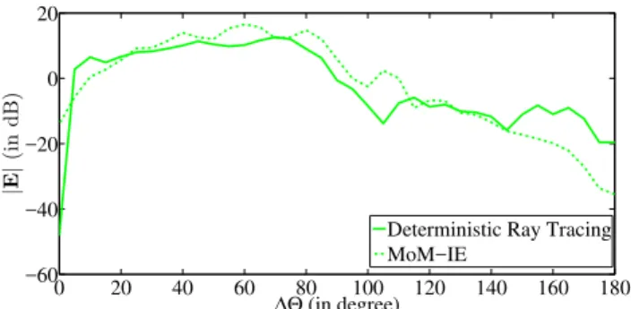
Fig. 9.Comparing the Ray Tracing and MoM-IE at the position of the green points in Fig. 8.
−80 −60 −40 −20 0 20 40 60 80
−30 −20 −10 0 10 20
∆Φ (in degree)
|
E
|
(in
d
B
)
Deterministic Ray Tracing MoM−IE
Fig. 10.Comparing the Ray Tracing and MoM-IE at the position of the red points in Fig. 8.
green points are located in the upper half-plane ofY =0 in every 5 degrees on a circle with the radius of 250 mm and center of(X, Y, Z)=(0,0,0). The red points are located in
Z=100 mm plane on a half circle with radius of 150 mm and center of(X, Y, Z)=(0,0,100). The result of this com-parison is presented in Figs. 9 and 10.
Comparing in both cases shows that the result of ray trac-ing stays in a good agreement with MoM-IE technique in the illumination and transition regions. In deep shadow region, ray tracer does not follow the same trend which results up to 10 dB difference. Higher accuracies are achievable by adding more details in the cost of higher runtime. In our application, we need a fast qualitative field distribution in an electrically large area. In this respect, the code performs well by com-putation of the electrical field in about 30 000 points which cover the surrounding space. This runtime will increase lin-early with number of rays. However, the runtime does not depend on fineness of the geometry matrix. The latter feature is very helpful to increase the accuracy of computation.
5 Conclusions
In this work, a fast deterministic ray tracer technique with matrix-based approach was presented. It was coded for a simple geometry scenario, however, the main functions such as the simultaneous multiple root finder and shadow region detector are in their most general forms. This means with a priori knowledge of the number of needed rays, one may simulate the EM fields for any structure as the structure can be imported with a simple geometry boolean data matrix. Based on the simulation, one not only may investigate cover-age but also calculate the channel impulse response complete Doppler or FMCW radar scenarios. The most important ad-vantage of the code is the frequency-independent short time of computation which is needed for complex scenarios and scenarios including moving targets where many simulations should be carried out.
References
Eibert, T.: Iterative-Solver Convergence For Star And Loop-Tree Decompositions in Method-of-Moments Solutions of the Electric-Field Integral Equation, IEEE Antenn. Propag. M., 46, 80–85, doi:10.1109/MAP.2004.1374101, 2004.
Flores, S., Mayorgas, L., and Jimenez, F.: Reception Algorithms For Ray Launching Modeling of Indoor Propagation, in: Proceedings of IEEE Radio and Wireless Conference, 261–264, 1998. James, G. L.: Geometrical Theory of Diffraction For
Electromag-netic Waves, 3rd Edn., IET, 1986.
Ling, H., Chou, R.-C., and Lee, S.-W.: Shooting and Bouncing Rays: Calculating the RCS of an Arbitrarily Shaped Cavity, IEEE T. Antenn. Propag., 37, 194–205, 1989.
Noori, N., Shishegar, A., and Jedari, E.: A New Double Counting Cancellation Technique For Three-Dimensional Ray Launching Method, in: IEEE Antennas and Propagation Society Interna-tional Symposium, 2185–2188, 2006.
Tignol, J.-P.: Galois’ Theory of Algebraic Equations, 2nd Edn., World Scientific Publisher Co., 2004.