2-D ZO CRS STACK BY CONSIDERING AN ACQUISITION LINE
WITH SMOOTH TOPOGRAPHY
Pedro Chira-Oliva
1, Jo˜ao Carlos R. Cruz
2, German Garabito
3, Peter Hubral
4and Martin Tygel
5Recebido em 12 janeiro, 2005 / Aceito em 6 abril, 2005 Received on January 12, 2005 / Accepted on April 6, 2005
ABSTRACT.The land seismic data suffers from effects due to the near surface irregularities and the existence of topography. For obtaining a high resolution seismic image, these effects should be corrected by using seismic processing techniques, e.g. field and residual static corrections. The Common-Reflection-Surface (CRS) stack method is a new processing technique to simulate zero-offset (ZO) seismic sections from multi-coverage seismic data. It is based on a second-order hyperbolic paraxial traveltime approximation referred to a central normal ray. By considering a planar measurement surface, the CRS stacking operator is defined by means of three parameters, namely the emergence angle of the normal ray, the curvature of the normal incidence point (NIP) wave, and the curvature of the normal (N) wave. In this paper the 2-D ZO CRS stack method is modified in order to consider effects due to the smooth topography. By means of this new CRS formalism, we obtain a high resolution ZO seismic section, without applying static corrections. As by-products the 2-D ZO CRS stack method we estimate at each point of the ZO seismic section the three relevant parameters associated to the CRS stack process.
Keywords: CRS stack, smooth topography, measurement surface curvature, near-surface irregularities.
RESUMO.Os dados s´ısmicos terrestres s˜ao afetados pela existˆencia de irregularidades na superf´ıcie de medic¸˜ao, e.g. a topografia. Neste sentido, para obter uma imagem s´ısmica de alta resoluc¸˜ao, faz-se necess´ario corrigir estas irregularidades usando t´ecnicas de processamento s´ısmico, e.g. correic¸˜oes est´aticas residuais e de campo. O m´etodo de empilhamento Superf´ıcie de Reflex˜ao Comum, CRS (“Common-Reflection-Surface”, em inglˆes) ´e uma nova t´ecnica de processamento para simular sec¸˜oes s´ısmicas com afastamento-nulo, ZO (“Zero-Offset”, em inglˆes) a partir de dados s´ısmicos de cobertura m´ultipla. Este m´etodo baseia-se na aproximac¸˜ao hiperb´olica de tempos de trˆansito paraxiais de segunda ordem referido ao raio (central) normal. O operador de empilhamento CRS para uma superf´ıcie de medic¸˜ao planar depende de trˆes parˆametros, denominados o ˆangulo de emergˆencia do raio normal, a curvatura da onda Ponto de Incidˆencia Normal, NIP (“Normal Incidence Point”, em inglˆes) e a curvatura da onda Normal, N. Neste artigo o m´etodo de empilhamento CRS ZO 2-D ´e modificado com a finalidade de considerar uma superf´ıcie de medic¸˜ao com topografia suave tamb´em dependente desses parˆametros. Com este novo formalismo CRS, obtemos uma sec¸˜ao s´ısmica ZO de alta resoluc¸˜ao, sem aplicar as correic¸˜oes est´aticas, onde em cada ponto desta sec¸˜ao s˜ao estimados os trˆes parˆametros relevantes do processo de empilhamento CRS.
Palavras-chave: empilhamento CRS, topografia suave, curvatura da superf´ıcie de medic¸˜ao, irregularidades pr´oximas da superf´ıcie.
1 Universidade Federal do Par´a, Departamento de Geof´ısica, Rua Augusto Corrˆeia 1, Campus Universit´ario do Guam´a, Caixa Postal 1611 – CEP 66017-970; Tel: (091) 3183-1473; Fax: (091) 3183-1671 – E-mail: [email protected]
2 Universidade Federal do Par´a, Departamento de Geof´ısica, Rua Augusto Corrˆeia 01, Campus Universit´ario do Guam´a, Caixa Postal 1611 – CEP: 66017-970; Tel: (91) 211-1473; Fax: (91) 211-1671 – E-mail: [email protected]
3 Universidade Federal do Par´a, Departamento de Geof´ısica, Rua Augusto Corrˆeia 01, Campus Universit´ario do Guam´a, Caixa Postal 1611 – CEP: 66017-970; Tel: (91) 211-1473; Fax: (91) 211-1671 – E-mail: [email protected]
4 Universidade de Karlsruhe, Instituto de Geof´ısica, Hertzstr. 16, D-76187 Karlsruhe, Alemanha. Tel: +49-(0)721-608-4443/4567; Fax: +49-(0)721-71173 – E-mail: [email protected]
INTRODUCTION
In order to obtain a high-resolution image of the earth sub-surface the geophysicists use the multi-coverage seismic data acquisi-tion, that yields to overlap registers of geological targets. In time domain, the ZO section is the seismic image obtained by con-sidering coincident sources and receivers. This is simulated by stacking the amplitudes using a traveltime operator, which is de-fined by means of stack parameters.
By the conventional seismic processing, the ZO section is simulated using the well-known normal moveout/dip moveout (NMO/DMO) stack method. Mann et al. (1999) presented a new stack method, so-called Common-Reflection-Surface (CRS), ba-sed on a hyperbolic second-order paraxial approach. By consi-dering a planar measurement surface, it depends on three para-meters, namely, the emergence angleβoof the normal ray, the
curvaturesKN I P andKN of the two hypothetic wavefront,
so-called NIP and N waves, respectively (Hubral, 1983).
Land seismic data are in general affected by the existence of surface topography and irregularities in the near-surface (e.g. weathering base and weathering velocity). In the conventional seismic processing, these effects are interpreted by deviations from hyperbolic NMO correction in the common-midpoint (CMP) gather. The topography effects are corrected by using field and residual static corrections. By applying specifically the field static correction, based on refraction seismic data, we remove the most part of these traveltime anomalies. Nevertheless, this correction usually does not account for rapid changes of the topography, in the weathering base, and of the weathering velocity. It is very sen-sitive to the choice of parameters involved in the picking phase.
According to Guo & Fagin (2002), land surveys should always be processed considering a floating datum that represents the to-pography. They showed that velocity analysis from a flat seismic reference datum creates errors to estimate the depth and interval velocities, even in the case of a flat topography, due to deviations of the take-off angles of the seismic ray paths.
Chira-Oliva & Hubral (2003) studied the sensibility of the interval velocity and reflector depth by considering a hypothetical circle measurement surface. They showed the NMO velocity by considering the curvature of the earth surface is more accurate to recover the interval velocities and the depths of the reflectors than the NMO velocities obtained by using a planar measurement surface approach. Chira-Oliva & Hubral (2003) and Zhang et al. (2002), respectively, presented the 2-D ZO CRS formalism for measurement surface with smooth and rugged topography. Chira-Oliva et al. (2001) modified the 2-D ZO CRS operator for
inclu-ding effects of near-surface inhomogeneity. In this paper, the 2-D ZO CRS stack performance is tested by considering a multi-layer model with smooth topography.
THEORY
The 2-D ZO CRS stacking operator depends on three parameters of two hypothetical waves, namely the normal-incidence-point (NIP) and Normal (N) waves (Hubral, 1983). These parameters are the emergence angle of the normal ray, and the radii of curvatures of the NIP and N waves. The emergence point,X0, of the normal ray
is called central point. The NIP wave propagates upwards from a point source located at the normal ray incidence point; and the N wave propagates upwards starting at the reflector, like an explo-ding reflector source.
Based on the hyperbolic second-order paraxial traveltime ap-proach, the 2-D ZO CRS stacking operator with smooth topo-graphy is given by (Chira-Oliva et al., 2001),
t2(xm,h)=
t0+2
sinβ0∗
v1
(xm−x0)
2
+2t0
v1
cos2β∗
0
RN
−cosβ0∗K0
(xm−x0)2
+2t0
v1
cos2β∗
0
RN I P
−cosβ∗ 0 K0
h2.
(1)
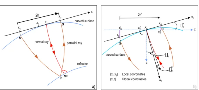
Equation (1) describes the reflection timet of the paraxial ray
S P Gin the vicinity of a normal (ZO) ray X0 N I P X0
(Fi-gure 1a). The ZO travel-time and the central point coordinate are
t0andx0, andv1is the near-surface velocity of the P-P wave at
the central pointX0. The coordinatesxmandhare, respectively,
the midpoint and half-offset referred to thex1-axis, that is
tan-gent to the topography surface with origin at the central pointX0
(see Figures 1a,b). The emergence angle of the normal ray at the central point isβ∗
0. The parameterK0is the local curvature of
the earth surface at a point of the acquisition line, that is positive (or negative) if this line falls below (or above) its tangent at X0.
The radii of curvatures of the emergence hypothetical NIP and N wavefronts atX0areRN I PandRNrespectively.
In order to normalize the processing coordinates, we apply a transformation from the local(x1,x3)into the global cartesian
system(x,z)in Figure 1b. The midpoint and half-offset coordi-nates,(xm,h)and(xm′ ,h
′), in the local and global coordinate
cartesian systems, respectively, are related by the expressions
h= h
′
cosα∗
0
, xm= x′
m
cosα∗
0
X0
Figure 1– a) Ray diagram for a paraxial ray in the vicinity of a normal ray in a 2-D laterally inhomogeneous medium. Local coordinates system(x1,x3)for a curved
measurement surface referred to pointX0. b) Transformation of the local coordinates,xmandh, to its global coordinatesxm′andh′. The local dip angle of the
tangent atX0(x1-axis) is defined byα0∗. The angle between the normal ray and the vertical line throughX0(z-axis) isβ0, andβ0∗is the angle between the normal
ray and the normal to the tangent atX0.
whereα∗
0 is the dip angle of the tangent x1-axis at point X0.
Introducing the relationships (2) into equation (1), we find
(e.g. Chira-Oliva & Hubral, 2003; Chira, 2003)
t2(x′m,h′)=
t0+2 sinβ0
∗
v1cosα∗0
(xm′ −x0)
2
+ 2t0 v1cos2α∗0
cos2β∗
0
RN
−cosβ0∗K0
(x′m−x0)2
+ 2t0 v1cos2α∗0
cos2β0∗
RN I P
−cosβ0∗K0
(h′)2.
(3)
We now consider apure diffraction, i.e., the situation in which the reflector reduces to a single diffraction point. In this case, the NIP and N waves are coincident, i.e. both propagate from a point source at NIP and have identical radii of curvatures atX0,RN ≡RN I P.
As a consequence, equation (3) becomes
tdi f f2 (xm′ ,h′)=
t0+2
sinβ0∗
v1 cosα∗0
(xm′ −x0)
2
+ 2t0
v1cos2α0∗
cos2β∗
0
RN I P
−cosβ0∗ K0
(xm′ −x0)2+(h′)2
.
(4)
Equation (4) depends on two CRS parameters(RN I P, β∗ 0)
associated to the NIP wave. This equation will be used at the first step of the CRS strategy. The CRS stacking operator defined by equation (4) is interpreted as an approach of the pre-stack Kir-chhoff migration operator with smooth topography.
Setting the conditionh′
=0to the general hyperbolic travel-time equation (3), the CRS stacking operator for reflected events
in the ZO configuration becomes
tZ O2 (x′
m)=
t0+2
sinβ0∗
v1 cosα0∗
(x′
m−x0)
2
+ 2t0
v1cos2α∗0
cos2β∗
0
RN −cosβ
∗ 0 K0
(xm′ −x0)2.
Following Garabito et al. (2001) the three optimal CRS pa-rameters(β∗
0,RN I P,RN)are searched by three steps. At the
first step we use formula (4) to determineβ∗
0 andRN I P. At the
second step we use formula (5) to determineRN; and at the third
step we use formula (3) to refine the three parameters.
2-D ZO CRS STACK
In the 2-D situation, for each pointP0(x0,t0)at the ZO section
to be simulated, the amplitudes in the seismic data will be sum-med (stacked) along the CRS surface defined by equation (3). The resulting (stacked) amplitude is assigned to the pointP0.
The three CRS stacking parameters are estimated by means of an optimization process, having the semblance as objective function. The CRS stacking optimization problem consists of estimating the parameters that maximize the semblance. In ge-neral, the problem requires a combination of multi-dimensional global and local optimization algorithms. The mathematical in-tervals defined for the parameters are−π/2 < β∗
0 < π/2,
−∞< RN I P,RN <∞. Optimization strategies to estimate
these parameters are found in the literature (e.g. M¨uller (1999); Birgin et al. (1999); Garabito et al. (2001)).
In this paper, we apply the strategy given by Garabito et al. (2001) to estimate the CRS parameters triplet, but using the new equations (3), (4) and (5).
CRS STACK PROCESSING STRATEGY
The proposed strategy to carry out the CRS method involves a combination of global and local search processes and is divided into three steps. The curvature,K0, of the seismic line at each
central point is supposed to be a priori known or calculated by means of some interpolation method by using elevation values. At the first and second steps we used the Simulated Annealing (SA) algorithm (Sen & Stoffa, 1995), and at the third step the Quasi-Newton (QN) algorithm (Bard (1974); Bard (1981)). Each step is performed on each sample pointP0(x0,t0)that pertains to the
ZO section to be simulated. The objective function is the sem-blance calculated for each point in the ZO section.
Step I: Pre-Stack Global Optimization
The multi-coverage pre-stack seismic data is the input. The in-verse problem consists of simultaneously estimating the two pa-rametersβ∗
0 and RN I P that provide the maximum semblance
value, according equation (4). The results of this step are: 1) ma-ximum coherence section, 2) emergence angle, β∗
0- section,
3) NIP-wave radius of curvature, RN I P-section, and 4)
simu-lated (stacked) ZO section.
Step II: Post-Stack Global Optimization
The post-stack seismic data is the input. The inverse problem consists of estimating the single parameter, RN, that provides the maximum semblance according to equation (5), in which the previously obtained parameter,β∗
0, is kept fixed. In this step the
results are: 1) maximum coherence section, 2) N-wave radius of curvature,RN-section, and 3) re-stacked simulated ZO (stacked)
section.
Step III: Pre-Stack Local Optimization
The multi-coverage pre-stack seismic data from step I is the input. The inverse problem consists of estimating the best parameter tri-plet(β∗
0,RN I P,RN)that provides the maximum semblance. In
this case the CRS stacking operator is equation (3), applied to the full multi-coverage data set with suitable apertures. In this step the results are: 1) maximum coherence section, 2) optimizedβ∗
0
-section, 3) optimizedRN I P-section, 4) optimizedRN-section, and 5) optimized ZO (stacked) section.
Example
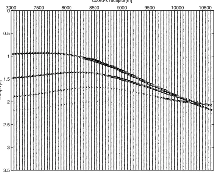
In order to test the CRS stacking algorithm we applied it to a synthetic data set computed for 2-D homogeneous layered mo-del shown in Figure 2. The momo-del is constituted of four layers above a half-space. The acquisition system is lying on a smooth topography line. Based on this model, we generated a synthe-tic data set of multi-coverage primary reflections, using the ray-tracing algorithm, SEIS88 ( ˇCerven´y & Psensik, 1988). In order to test the accuracy of the CRS method, it was added random noise with signal-to-noise ratio ofS/N = 10. The data set consis-ted of 201 common-shots (CS) with 72 receivers with interval of 50 meters. The minimum offset was 50 meters. The source signal was a Gabor wavelet with 40 Hz dominant frequency and the time sampling was 4 ms. An example of part of these data is presented in Figure 3, represented by a CS section.
Figure 2– 2-D model constituted of four isovelocity layers about a half-space with curved interfaces and curved measurement surface. Interval velocities are 1.75 km/s, 2.4 km/s, 3.5 km/s, 4.65 km/s and 5.5 km/s, respectively.
7000 7500 8000 8500 9000 9500 10000 10500
0
0.5
1
1.5
2
2.5
3
3.5
Tempo [s]
Coord-x receptor[m]
Figure 3– Example of a CS section of multi-coverage pre-stack seismic data of the model of Figure 2. The ratio signal/noise is 10.
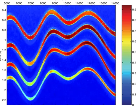
maximum coherence (semblance) section that corresponds to the best parameters. We note that the coherence values become smal-ler for larger traveltimes (deeper events). Figures 7, 8 and 9 show the sections of emergence angle and radii of curvature of the NIP and N waves, respectively. These sections correspond to global maxima determined at the third step.
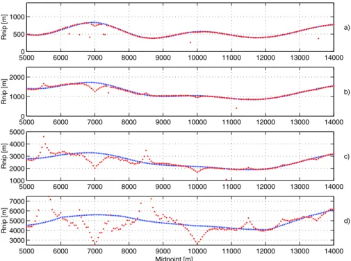
A comparison between the emergence angles,β∗
0, estimated
by the CRS algorithm (curves of red points) and by modelling (curves of blue points), respectively, is shown in Figure 10. We can see the emergence angle has been well estimated along all reflectors. Figures 11 and 12 show the analogous comparison for the other parameters,RN I PeRN, respectively. These
Midpoint [m]
T
im
e
[
s
]
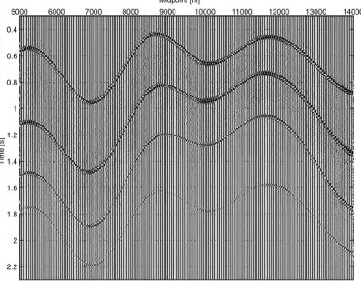
Figure 4– ZO section with random noise (ratio S/N = 10) obtained by forward modelling.
5000 6000 7000 8000 9000 10000 11000 12000 13000 14000
0.4
0.6
0.8
1
1.2
1.4
1.6
1.8
2
2.2
Time [s]
Midpoint [m]
Figure 5– Simulated ZO section with the ZO CRS stack by using the multi-coverage seismic data with random noise (ratio S/N = 10).
CONCLUSIONS
A new formula for the CRS stack method that considers the smo-oth topography of the acquisition line has been tested in synthetic data sets with successful results. The parameters were correctly estimated, excepting the regions where there are abrupt changes of the curvature of the topography line. In these regions, the er-rors of the estimated parameters increase with depth. Besides the simulated ZO sections, we have obtained the coherence section
and the sections referred to the attributes of the NIP and N waves.
ACKNOWLEDGMENTS
0 0.1 0.2 0.3 0.4 0.5 0.6 0.7 0.8 0.9 Midpoint [m]
Time [s]
5000 6000 7000 8000 9000 10000 11000 12000 13000 14000
0.4
0.6
0.8
1
1.2
1.4
1.6
1.8
2
2.2
Figure 6– CRS optimized coherence section of the model of Figure 2.
−50 −40 −30 −20 −10 0 10 20 30 40 50 Midpoint [m]
Time [s]
5000 6000 7000 8000 9000 10000 11000 12000 13000 14000 0
0.5
1
1.5
2
2.5
Figure 7– CRS optimizedβ∗
0 1000 2000 3000 4000 5000 6000 7000 Midpoint [m]
Time [s]
5000 6000 7000 8000 9000 10000 11000 12000 13000 14000 0
0.5
1
1.5
2
2.5
Figure 8– CRS optimizedRN I P-section of the model of Figure 2.
−30000 −20000 −10000 0 10000 20000 30000 Midpoint [m]
Time [s]
5000 6000 7000 8000 9000 10000 11000 12000 13000 14000 0
0.5
1
1.5
2
2.5
5000 6000 7000 8000 9000 10000 11000 12000 13000 14000 −20
0 20
Angle [graus]
a)
5000 6000 7000 8000 9000 10000 11000 12000 13000 14000 −40
−20 0 20 40
Angle [graus]
b)
5000 6000 7000 8000 9000 10000 11000 12000 13000 14000 −40
−20 0 20 40
Angle [graus]
c)
5000 6000 7000 8000 9000 10000 11000 12000 13000 14000 −40
−20 0 20 40
Midpoint [m]
Angle [graus]
d)
Figure 10– Comparison between CRS (curve of red points) and model-derived (curve of blue points) emergence anglesβ∗0. The parameter for each interface are plotted separately: a) first, b) second, c) third and d) fourth interface of the model of Figure 2.
50000 6000 7000 8000 9000 10000 11000 12000 13000 14000 500
1000
Rnip [m]
a)
50000 6000 7000 8000 9000 10000 11000 12000 13000 14000 1000
2000
Rnip [m]
b)
5000 6000 7000 8000 9000 10000 11000 12000 13000 14000 1000
2000 3000 4000 5000
Rnip [m]
c)
5000 6000 7000 8000 9000 10000 11000 12000 13000 14000 3000
4000 5000 6000 7000
Midpoint [m]
Rnip [m]
d)
Figure 11– Comparison between CRS (curve of red points) and model-derived (curve of blue points) radius of curvature,RN I P.
5000 6000 7000 8000 9000 10000 11000 12000 13000 14000 −5
0 5x 10
4
Rn [m]
a)
5000 6000 7000 8000 9000 10000 11000 12000 13000 14000 −5
0 5x 10
4
Rn [m]
b)
5000 6000 7000 8000 9000 10000 11000 12000 13000 14000 −5
0 5x 10
4
Rn [m]
c)
5000 6000 7000 8000 9000 10000 11000 12000 13000 14000 −5
0 5x 10
4
Midpoint [m]
Rn [m]
d)
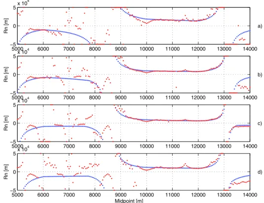
Figure 12– Comparison between CRS (curve of red points) and model-derived (curve of blue points) radius of curvature,RN.
The parameter for each interface are plotted separately: a) first, b) second, c) third and d) fourth interface of the model of Figure 2.
5 6 7 8 9 10 11 12 13 14
−1 −0.5 0 0.5 1
xm (km)
Ko (km
−1
)
Figure 13– Curvature of measurement surface along the acquisition line. It presents the points of abrupt changes of the curvature of the model of Figure 2.
REFERENCES
BARD B. 1974. Nonlinear parameter estimation: Academic Press.
BIRGIN E, BILOTI R, TYGEL M & SANTOS LT. 1999. Restricted opti-mization: a clue to a fast and accurate implementation of the common reflection surface stack. Journal of Applied Geophysics, 42: 143–155.
ˇCERVEN´Y V & PSENSIK I. 1988. Ray tracing program. Charles Univer-sity, Czechoslovakia.
CHIRA P. 2003. Empilhamento pelo m´etodo Superf´ıcie de Reflex˜ao
Co-mum 2-D com topografia e introduc¸˜ao ao caso 3-D. Ph.D. thesis, Federal University of Par´a, Brazil.
CHIRA-OLIVA P & HUBRAL P. 2003. Traveltime formulas of near-zero-offset primary reflections for a curved 2-D measurement surface. Geo-physics, 68(1): 255–261.
GARABITO G, CRUZ JC, HUBRAL P & COSTA J. 2001. Common Reflec-tion Surface Stack: A new parameter search strategy by global optimiza-tion. 71th. SEG Mtg., Expanded Abstracts. San Antonio, Texas,USA.
GILL PE, MURRAY W & WRIGHT MH. 1981. Practical optimization: Aca-demic Press.
GUO N & FAGIN S. 2002. Becoming effective velocity-model builders and depth imagers, part 2 – the basics of velocity-model building, examples and discussions Multifocusing. The Leading Edge, pages 1210–1216.
HUBRAL P. 1983. Computing true amplitude reflections in a laterally inhomogeneous earth. Geophysics, 48: 1051–1062.
MANN J, J¨AGER R, M ¨ULLER T, H ¨OCHT G & HUBRAL P. 1999.
Common-reflection-surface stack – A real data example. Journal of Applied Geo-physics, 42: 301–318.
M ¨ULLER T. 1999. The common reflection surface stack method – seismic imaging without explicit knowledge of the velocity model. Ph.D. Thesis, University of Karlsruhe, Germany.
SEN M & STOFFA P. 1995. Global optimization methods in geophysical inversion. Elsevier, Science Publ. Co.
ZHANG Y, H ¨OCHT G & HUBRAL P. 2002. 2D and 3D ZO CRS stack for a complex top-surface topography. Expanded Abstract of the 64th EAGE Conference and Technical Exhibition.
NOTES ABOUT THE AUTHORS
Pedro Chira-Oliva.He received his diploma in Geological Engineering (UNI-Peru/1996). He also received his MSc in 1997 and PhD in 2003, both in Geophysics, from Federal University of Par´a (UFPA/Brazil). He took part of the project of scientific research “3D Zero-Offset Common-Reflection-Surface (CRS) stacking” (2000-2002), sponsored by Oil Company ENI (AGIP Division – Italy) and the University of Karlsruhe (Germany). Since 2003 he is researcher of the UFPA, responsible for the scientific project “Generalization of the Common-Reflection-Surface (CRS) stacking applied to real data in the Amazon region”, financed by the PROSET/CT-PETRO/CNPq. He is an associate member of the Society of Exploration Geophysicists (SEG), Brazilian Geophysical Society and also is member of the Wave Inversion Technology (WIT) Corsortium (Germany).
Jo˜ao Carlos Ribeiro Cruz.He received a BS (1986) in Geology, MS (1989) and Ph.D. (1994) in Geophysics from the Federal University of Par´a, Brazil. From 1991 to 1993 was with the reflection seismic research group of the University of Karlsruhe, Germany, while developing PhD thesis. Since 1996 he has been a full professor at the Geophysical Department of the Federal University of Par´a (UFPA). Since 1999 he has been Dean of the Geophysical Graduate Scholl at UFPA. His current research interests include velocity analysis, seismic imaging, and apllication of inverse theory to seismic problems. He is a member of SEG, EAGE and SBGf.
German Garabito.He received his BSc (1986) in Geology from University Tom´as Frias (UTF), Bolivia, his MSc in 1997 and PhD in 2001 both in Geophysics from the Federal University of Par´a (UFPA), Brazil. Since 2002 he has been full professor at the geophysical department of UFPA. His research interests are data-driven seismic imaging methods such as the Common-Refection-Surface (CRS) method and velocity model inversion.
Peter Hubral.He obtained his MSc in Geophysics (Clausthal/1967) and Ph.D. in Geophysics (Imperial College London/1970). He is Professor at the University of Karlsruhe since 1986, having lectured at PPPG-UFBa (Salvador/1983-1984), Institute of Geophysics at University of Pau (France/1985-1986) and UFPa (2002-2003). He received the awards:Schlumberger (EAGE/1978), Erasmus (EAGE/2003), Reginald Fessenden (SEG/1979), Professor estrangeiro (SBGf/1999). He is a honorary member of SEG (1979) and EAGE (2002). He coordinates the Wave Inversion Technology (WIT) Cosortium and is director of the Institute of Applied Geophysics at Karlsruhe (Germany).