Job search, conditional treatment and recidivism: the employment services for exoffenders program reconsidered

(1)

Job Search, Conditional Treatment and

Recidivism: The Employment Services for

Ex-Oﬀenders Program Reconsidered

Herman J. Bierens

∗

Department of Economics, Pennsylvania State University

José R. Carvalho

†

CAEN, Universidade Federal do Ceará, Brazil.

October 29, 2007

Abstract

The objective of this paper is to re-evaluate the effect of the 1985 ”Em-ployment Services for Ex-Offenders” (ESEO) program on recidivism, in San Diego, Chicago and Boston. The initial group of program par-ticipants was split randomly in a control group and a treatment group. The actual treatment (mainly being job related counseling) only takes place conditional on finding a job, and not having been arrested, for those selected in the treatment group. We use interval-censored pro-portional hazard models for job search and recidivism time, where the latter model incorporates the conditional treatment effect, depending on covariates. Wefind that the effect of the program depends on loca-tion and age. The ESEO program reduces the risk of recidivism only for ex-inmates over the age of 27 in San Diego and Chicago, and over the age of 36 in Boston, but increases the risk of recidivism for the other ex-inmates in the treatment group.

∗_{Correspondence address: Herman J. Bierens, Department of Economics,} Pennsylva-nia State University, 608 Kern Graduate Building, University Park, PA 16802. E-mail: hbierens@psu.edu.

†_The _ﬁ_{nancial support of CAPES Foundation, Brazil, is gratefully acknowledged.}

(2)

Key words: Job search, Recidivism, Conditional treatment, Program evaluation, Duration models, Interval-censoring.

1 Introduction

Accordingly to Bloom (2006), more than 600,000 people are released from prison each year in the United States. By any standards this fact raises many concerns about the likely consequences, both social and economic, of such a massive inﬂux of ex-convicts into society. A prominent issue nowadays is the high rates of recidivism prevalent in the country, despite the huge eﬀorts by public authorities to make sure that the rehabilitative role of prisons works properly. In fact, recidivism rates measured by the Bureau of Justice Statistics (1994) show that two-third of released prisoners are re-arrested and one-half are re-incarcerated within three years after release. After a decade from release, Freeman (2003) asserts that, after a decade from release, up to 80% of prisoners are re-arrested.

Most ex-offenders have low educational levels, medical problems, less work experience than non-offenders. Therefore, the prospects of ex-offenders in the job market are almost always worse than for non-offenders with com-parable characteristics (Freeman 1999 and Western 2002), although this is also true before incarceration. This means that incarceration may not be the only reason for low job market performance; the characteristics that caused the conviction could have caused the bad performance in the labor market as well.

The idea that having a job diminishes the chances of recidivism is well established in the criminological literature. See Sampson and Laub (1997) and Harer (1994). A job provides the necessary means for survival, improves self-esteem, increases the attachment to a community and develops the sense of belonging to a group. Therefore, even though finding a job is a difficult task for ex-offenders, a policy that help these people to find a job will likely decrease the chances of recidivism.

(3)

employment programs. However, as outlined by Bloom (2006), ”there appear to have been few rigorous studies of employment-focused re-entry models”. Moreover, Farrington and Welsh (2005) state that very few evaluations in criminology can be classiﬁed as rigorous, in that they are not randomized experiments. Furthermore, it appears that in the criminological literature a randomized experiment is considered synonym for a program with random-ized treatment.

During the last decades, sociologists, criminologists and, to a lesser ex-tent, economists have been devising programs to ease the difficult transition faced by ex-offenders during the period of time between release and reinte-gration into society. These programs are basically of two types: post-release programs and in-prison programs. While the former type of program offers assistance after the individual has been released, the latter type of program starts helping the individual while he/she is in prison. As experience has accumulated, a fundamental goal to a complete reintegration turned out to be job placement. A good job would be necessary not only to provide the basic needs for survival in the short run but also as a key element to secure self-esteem, security and sense of integration in the society as whole.

The Life Insurance for offenders and the Transitional Aid for Ex-offenders are two early examples of employment services for ex-Ex-offenders. Both programs offeredfinancial assistance as well as job placement services. The two programs reached similar conclusions: while financial assistance appeared to decrease the recidivism rate, job placement had little or no effect on reducing criminal activity, unless for those who succeeded in securing a job for a long time. The lack of follow-up after placement was conjectured by Milkman et al. (1985) as the main obstacle to the complete success of such programs.

The new paradigm of employment services for ex-offenders have resulted in the appearance of programs that had a strong preoccupation with the post-placement of their clients. These programs have designed follow-up strategies to overcome the major criticism of past experience. Among vari-ous programs, three deserve recognition for both being successful and having similar structures: the Comprehensive Offender Resource System (COERS) in Boston, the Safer Foundation (SF) in Chicago and Project JOVE in San Diego. Not surprisingly, the US Department of Justice saw this as a op-portunity for assessing the efficacy of employment services programs that contained a follow-up component.

(4)

spon-sored a controlled experiment to evaluate the impact of reemployment pro-grams for recent released prisoners. This evaluation was performed by the Lazar Institute in McLean, Virginia. The three aforementioned programs, COERS in Boston, JOVE in San Diego and SF in Chicago, were chosen to participate in the Employment Services for Ex-Oﬀenders Program, hence-forth ESEO. A total of 2045 prisoners who volunteered to participate in the program were randomly assigned to either a treatment group or a control group. Those in the ﬁrst group received, besides the normal services (ori-entation, screening, evaluation, support services, job development seminar, and job search coaching), special services which consisted of an assignment to a follow-up specialist who provided support during the job search and the

180 days following job placement. The control group received only normal services.

Using OLS regressions, Milkman (2001) found that the eﬀect of the ESEO special services program is negligible. However, this evaluation did not ac-count for the conditional feature of the treatment. The timing of the treat-ment was completely neglected, which is a very important characteristic of the program under evaluation.

The objective of our paper is to re-evaluate the effect of the ESEO pro-gram on recidivism using duration models for job search and recidivism (the latter being defined as the time between release and the first arrest), with the conditional treatment incorporated in the latter duration model. These two durations are interval censored, though.

Carvalho and Bierens (2007) have studied the eﬀect of the ESEO program on recidivism using a bivariate mixed proportional Weibull hazard model for job search and recidivism with common heterogeneity, where both durations are assumed to be independent conditional on the covariates and the het-erogeneity variable. The latter is assumed to be Gamma distributed, and integrated out to make the two durations dependent conditional on the co-variates only. However, the problem with this approach is that then the job search and recidivism durations are positively related: The longer the job search takes, the longer the time between release and rearrest. This is clearly unrealistic.

(5)

den Berg (2003).1 _{These authors propose a bivariate mixed proportional}

hazard model, where one duration is the timing of the treatment and the other one is the duration of interest that is aﬀected by the treatment. In the case of the ESEO program the duration that triggers the treatment is the job search, and the duration of interest is recidivism. However, since both durations are interval-censored and all the covariates are discrete we cannot take unobserved heterogeneity into account, because it is shown in Bierens (2007) that then the mixed proportional hazard model is not identiﬁed.

The setup of the paper is as follows. In Section 2 we discuss the ESEO program in more detail, and we describe the data set and the variables in-volved. Section 3 deals with the attrition problem, which is substantial. It appears that attrition is affected by the group assignment: the attrition rate is higher for the control group than for the treatment group. In Section 4 we conduct a preliminary data analysis by nonparametrically estimating and comparing the interval probabilities for both durations without using covariates, in order to check for evidence of dependence of recidivism on job search, and evidence of a treatment effect. We find neither, and therefore we conclude that at least for the control group the job search and recidivism durations are independent conditional on the covariates, and that if there is a treatment effect then it will likely work via covariates. Section 5 deals with model specification and estimation. In Section 5.1 we discus the Abbring and Van den Berg (2003) model and its relation to our model. In Section 5.2 we estimate and test an interval-censored proportional hazard model for the job search, where in first instance the integrated hazard is left unspecified. Only the location (Chicago, San Diego or Boston) seems to matter for the job search duration, and the results indicate that a Weibull baseline hazard is appropriate for job search. Similarly, in Section 5.3 we estimate and test an interval censored proportional hazard model for the recidivism duration of the control group only. It appears that none of the covariates matter and that the baseline hazard is constant, hence the distribution involved is ex-ponential. In Section 5.4 we extend this exponential model for recidivism to a model that incorporates treatment via covariates, depending on the job search duration, and merge it with the job search model, which are then es-timated jointly by maximum likelihood. The results are presented in Section 5.5. It appears that a treatment effect is present, but its magnitude and direction depends on the location and on age. In Section 5.6 we compute

(6)

the actual treatment effect, in terms of expected increase or reduction of the recidivism duration in months, on the basis of our estimations results. In Section 5.7 we compare the results with the preliminary data analysis, and explain why we did not find in first instance evidence of dependence of the job search and recidivism durations and the presence of a treatment effect. In Section 6 we summarize our results and make recommendations for future setup and evaluations of employment programs for ex-offenders. Section 7 is an appendix containing the details of the model selection procedures.

The econometric analysis in this paper has been conducted using the free econometric software package EasyReg International developed by the ﬁrst author. See Bierens (2006).

2 The ESEO program and data set

2.1 The ESEO Program

In the ESEO program, after being assigned randomly to either the control or treatment group, the clients enter the intake unit, where they receive initial orientation, screening and evaluation by an intake counsellor. While still in this first phase, to secure survival up to the job search phase, the intake counsellor offers assistance services such as food, transportation, and cloth-ing. After intake, the clients enter the second phase that will prepare them to develop job search skills. In particular, a brief job development seminar is offered which deals with issues like appropriate dress and deportment, typical job rules, goal setting, interviewing techniques, and job hunting strategy. It is assumed that the time spent in the first and second phases are negligible compared to the job search phase. The next and final phase before possible treatment is the job search assistance. This is the traditional job search as-sistance type of service, as described by Bloom (2006) and Heckman et al. (1999). The job search assistance in the ESEO program is offered equally to both control and treatment groups.

(7)

of the programs and treatment. Thus, even though the split of the sample in treatment group and control group is random, the actual treatment is the follow-up special services afterﬁnding a job and is therefore not randomized.

2.2 The ESEO data

The ESEO data set consist of 2045 individuals who participated in one of the three programs: 511 in Boston, 934 in Chicago and 600 in San Diego. However, the ICPSR2 _{only made available} ₁₀₇₄_{usable observations}3_: ₃₂₅_in

Boston,489in Chicago and260in San Diego. A large amount of information, sometimes very detailed, was collected from all three sites.

Aﬁrst important empirical issue is related to the characterization of the population being sampled. Unless very special assumptions are made, the validity of ourﬁndings can not be extrapolated beyond the population under sampling. In order to be eligible to participate in the ESEO program an individual must have the following background:

1. Participants voluntarily accepted program services;

2. Participants had been incarcerated at an adult Federal, State, or local correctional facility for at least 3months and had been released within

6 months of program participation;

3. Participants exhibited a pattern of income-producing oﬀenses.

From the eligibility criteria it is clear that our population is a special, indeed a very special, subset of the population of ex-oﬀenders. Also, since participation is voluntary and there is no information on non-participants (those who did not choose to participate even though they fulﬁlled require-ments2and 3), it is not possible to assess the potential bias induced by this selection scheme.

2_{The data set used in our present analysis comes from the Inter-University Consortium} for Political and Social Research, henceforth ICPSR, University of Michigan, under the study number8619.

(8)

Given the initial sample, the individuals were randomly assigned to ei-ther the treatment or control group. Control group received the standard services and the treatments group received, in addition to that, emotional support and advocacy during the follow-up period of 180 days after place-ment. Two durations are of great importance, time spent searching a job and recidivism time. These two variables are interval-censored, however; they are only observed in the form of intervals. Moreover, there is a substantial num-ber of individuals in the sample who do not show up for the common part of the program, i.e., the assistance with the job search. Thus, the endogenous variables are:

• A: Indicator for attrition. A = 1 means the individual is either a “no show” or a “drop-out”, A= 0 otherwise;

• Ts (s=search)is the duration of the job search, i.e., the time between

the date of release and the date of placement in the ﬁrst job after release;

• Tc (c =crime) is the recidivism time, i.e., the time between the date

of release and the date of theﬁrst arrest after release.

As to attrition, one could argue that ”no show” and ”drop—out” deserve separate treatment, as pointed out by Bloom (1984) and Heckman et al. (1998). However, our data set does not allow for this disaggregation. Besides, most drop-outs occur very early in the program.

The job search duration does not need any explanation, but the mean-ing of ”recidivism” is not unambiguous. There are two ways to measure recidivism outcomes in the ESEO program, via count data or duration data. Detailed data on the number of arrests from date of released to the end of the program for all clients was gathered in the respective state police de-partments. That was the type of data used in the original evaluation made by Milkman et al. (1985), as well as in almost all literature regarding the evaluation of employment programs for ex-oﬀenders. See Visher et al. (2005) and Seiter and Kadela (2003).

(9)

of) recidivism” should be interpreted as the time between release and ﬁrst rearrest.

Although, from a methodological point view, the measure of recidivism by means of a duration complicates the model, we believe that this is the right way to proceed because: (a) it conforms to the notion that recidivism is a time interval of occurrence of a ﬁrst event; (b) unless very special parametric assumptions are made, the number of occurrences in a time interval can not be uniquely determined by a process describing the time of occurrence of the ﬁrst event, and vice-versa; (c) given the dynamic nature of the treatment, measuring the outcome of the program, i.e., recidivism time, as a duration variable has a much more natural appeal.

The point of departure for the choice of the covariates of the recidivism duration model is Schmidt and Witte (1988): age at release, time served for the sample sentence, sex, education, marital status, race, drug use, supervi-sion status, and dummies that characterize the type of recidivism. However, we have also paid close attention to the criminological literature in recidivism, for instance Gendreau et al. (1996).

The literature on unemployment (and job search) duration has been re-fined since the 70’s. Nowadays, it has a status of a complete theory of unem-ployment, as it appears in Pissarides (2000). Its empirical contents has been developed since the late 70’s and thisfirst wave of empiricism is characterized for being concerned with “reduced” type models. A good account of thisfirst phase can be found in Devine and Kiefer (1991). A final wave is character-ized by advocating a “structural” approach to estimation and inference in such models. An updated account of that appears in Van den Berg (1999, 2000). There has been also studies close to ours that try to measure the effect of programs in a context of a model of unemployment and job search duration. See for instance, Abbring and Van den Berg (2003), Abbring et al. (2005), Eberwein et al. (1997) and Van den Berg et al. (2004). In view of those studies, the following set of covariates has been singled out, next to the group assignment indicator:

• G= 1if selected in the treatment group, = 0 if selected in the control group

• DRU GS: Indicator for drugs use during the last 5 years;

(10)

• MALE: Gender indicator;

• EDUC L= 1 if years of schooling _≤8, = 0otherwise;

• EDUC H = 1 if years of schooling >12,= 0 otherwise;

• AGE: Age in years;

• AGE1ARR: Age of ﬁrst arrest, in years;

• SAN DIEGO: Indicator for San Diego;

• CHICAGO: Indicator for Chicago;

In the econometric model to be developed the job search and recidivism durations Ts andTc,respectively, are inﬁrst instance modeled as continuous

latent variables, where treatment kicks in for people in the treatment group if Tc > Ts. The treatment is eﬀective in reducing recidivism if, given the

same job search duration Ts and the covariates, the recidivism duration Tc

for the treatment group is larger than for the control group. Note that, since Tc < Ts is also possible, some people in the treatment group may end up not

receiving the treatment at all.

Finding a job may postpone recidivism, but will likely not eliminate it. As Freeman (2003) asserts, ”Getting and ex-oﬀender a job does not mean that they will eschew a criminal opportunity if it arises”. Thus, in our model the probability that Tc = ∞ is assumed to be zero. The use of continuous

latent variables advocated by us also appears to conform better with what is noted by Fagan and Freeman (1999) and Freeman (2003), namely that the boundary between crime and work is thin and very diﬀuse for many young men just after release. The two clocks, i.e., time to recidivism and time to get a job, are about to be pushed down every day for these young men.

Although the latent variables Ts and Tc will be modeled as a joint

con-tinuous distribution, conditional on covariates, we only observe them in the form of intervals: Ts ∈ (a, b], Tc ∈ (p, q], b ≤ p, where (a, b],(p, q] ∈

{(0,1],(1,6],(6,12],(12,_∞)}. The unit of measurement for these durations is months. These events are only observed if A = 0. Given the joint condi-tional distribution of Ts andTc,the probabilities of these discrete events can

be computed. The latter are then used to form a likelihood function.

(11)

get standard assistance with the job search. Treatment consists of extra help after ﬁnding a job, and is therefore conditional on the job search duration Ts. The purpose of this study is to determine whether this treatment has an

eﬀect on the risk of recidivism, given the covariates listed above.

3 Attrition

With a few exceptions, attrition occurs straight away after release. It is therefore reasonable to assume that, conditional on the covariates (stacked in a vector X), A is independent of Ts and Tc, because in most cases the

attrition decision A= 1is made before Ts orTc are realized.

The conditional attrition probability P[A = 1|X] has been modeled as a Logit model. It is conceivable that attrition is also affected by the group assignment: The prospect of receiving treatment (G = 1) may lead to a lower attrition probability. Therefore, next to the original covariates we have included the group assignment G and the products of G with each of the covariates in the Logit model for A. The initial Logit model has been subjected to a sequence of Wald and likelihood ratio tests to clean the model of insignificant covariates. The details of this cleaning process can be found in the Appendix; only the final results are presented, in Table 1.

Table 1. Logit results for attrition

Covariates Estimates t-val.

M ALE×(1−G) 0.7835337 3.93

CHICAGO×(1₋G) 1.7985664 7.94

CHICAGO×G 0.5250147 2.71

SANDIEGO×(1₋G) 1.0452205 3.55

SANDIEGO×G 0.4278509 2.05

1 ₋0.7661767 ₋5.26

Log-likelihood: ₋654.831

Sample size: 1074

It follows from Table 1 that males have a higher attrition rate than females, but only if selected in the control group. Moreover, the attrition rates in Chicago are signiﬁcantly higher for the control group than for the treatment group, and the same applies to San Diego.

(12)

dummies with the intercept, which leads to the conclusion that the attrition rates in Chicago and San Diego are much higher than in Boston, in particu-lar for the control group, and within the control group the attrition rate in Chicago is higher than in San Diego, although for the treatment group the attrition rates in Chicago and San Diego are not significantly different (the p-value of the Wald test involved is 0.62037). The reason may be that the standard service in assisting the ex-inmates with the job search is much more effective in Boston than in San Diego and Chicago, and that therefore the motivation for participation in the program is higher in Boston than in the other two cities. This explanation appears to be corroborated by the results below for the job search duration.

Finally, note that the dependence of attrition on the group assignment does not conﬂict with our assumption that conditional on the covariates Ts

and Tc are independent ofA, becauseG is determined randomly.

4 Preliminary data analysis

As said before, the durations Tc and Ts are only observed in the form of

interval indicators, for the intervals (0,1],(1,6],(6,12] and (12,_∞). Table 2 presents the number of observations in each interval and combination of intervals, for both groups as well as separately for the treatment group (G= 1) and the control group (G= 0).

By dividing the entries in rows 1-4 in Table 2 by the corresponding row totals we get nonparametric estimates of the conditional probabilities P [Tc ∈(p, q]|Ts ∈(a, b]],and in the last rows the unconditional probabilities

P [Tc ∈(p, q]]. These probabilities, times 100%, are presented in Table 3.

Comparing the entries in rows 1-4 of Table 3 with the corresponding entries in row 5, it appears that for both groups separately and together all but one of the estimates ofP [Tc ∈(p, q]|Ts ∈(a, b]]are close to the estimates

of P[Tc ∈(p, q]].The exception is the estimate ofP [Tc >12|Ts∈(6,12]]for

the control group, but this estimate is based on only two observations. For our analysis only the probabilities P [Tc ∈(p, q]|Ts∈(a, b]]forp≥b

are relevant. In the Appendix we present the results of tests of the null hypothesis that P [Tc ∈(p, q]|Ts ∈(a, b]] = P[Tc ∈(p, q]] for p ≥ b. In all

cases the null hypothesis is not rejected at any conventional signiﬁcance level! Therefore, it seems that the events Tc ∈ (p, q] and Ts ∈ (a, b] for b ≤ p are

(13)

Table 2. Observations per interval (A=0)

TsÂTc (0,1] (1,6] (6,12] (12,∞) T otal

(0,1] 12 56 43 152 263

(1,6] 6 44 39 112 201

(6,12] 1 7 6 20 34

(12,∞) 0 1 1 3 5

T otal 19 108 89 287 503

Treatment group only:

TsÂTc (0,1] (1,6] (6,12] (12,∞) T otal

(0,1] 9 39 32 105 185

(1,6] 5 35 30 81 151

(6,12] 1 4 5 18 28

(12,∞) 0 1 1 3 5

T otal 15 79 68 207 369

Control group only:

TsÂTc (0,1] (1,6] (6,12] (12,∞) T otal

(0,1] 3 17 11 47 78

(1,6] 1 9 9 31 50

(6,12] 0 3 1 2 6

(12,_∞) 0 0 0 0 0

(14)

Table 3. Estimated conditional probabilities

P[Tc ∈(p, q]|Ts∈(a, b]]×100%

TsÂTc (0,1] (1,6] (6,12] (12,∞)

(0,1] 5 21 16 58

(1,6] 3 22 19 56

(6,12] 3 20 18 59

(12,_∞) 0 20 20 60

(0,∞) 4 21 18 57

Treatment group only:

TsÂTc (0,1] (1,6] (6,12] (12,∞)

(0,1] 5 21 17 57

(1,6] 3 23 20 54

(6,12] 4 14 18 64

(12,_∞) 0 20 20 60

(0,∞) 4 21.5 18.5 56

Control group only (? = undeﬁned):

TsÂTc (0,1] (1,6] (6,12] (12,∞)

(0,1] 4 22 14 60

(1,6] 2 18 18 62

(6,12] 0 50 17 33

(12,_∞) ? ? ? ?

(15)

in the case G= 1these events are dependent.

These results are compatible with independence ofTc andTs conditional

on the covariates, provided that the vectorX of covariates can be partitioned as

X = (X_s0, X_c0)0, whereXs and Xc are independent, (1)

and

P[Ts≤t|X] =P [Ts≤ t|Xs], P[Tc ≤t|X] =P[Tc ≤ t|Xc]. (2)

Therefore, at least for the control group, we will assume that the conditions (1) and (2) hold.

If there is a treatment eﬀect, then fort > Ts,

P [Tc ≤t|Ts, Xc]=6 P[Tc ≤ t|Xc], (3)

so that for the treatment group,

P [Tc ∈(p, q], Ts∈(a, b]] =P [Tc ∈(p, q]]P [Ts∈(a, b]]

+ Z b

a

(P [Tc ∈(p, q]|Ts=ts]−P[Tc ∈(p, q]])dP [Ts ≤ts].

If the latter term is small then the events Tc ∈ (p, q] and Ts ∈ (a, b] are

approximately independent. Thus, if the dependence of P [Tc ≤t|Ts, Xc]on

Ts is substantially reduced after Xc is integrated out, then the inequality

(3) may no longer be detectable. Therefore, a treatment eﬀect may still be possible, but if so it will likely work via the covariates X.

5 Modeling strategy and empirical results

5.1 The Abbring-Van den Berg model

Abbring and Van den Berg (2003) consider the problem of identiﬁcation of treatment eﬀects in a bivariate mixed proportional hazard model, where one duration, S, is the timing of an intervention on another duration Y. In their Model 1a they specify the hazard functions of these duration as

(16)

for the durationS and

θS(t|S, X, V) = ½

λY(t)ϕY(X)VY if t≤ S

λY(t)ϕY(X)δ(t|S, X)VY if t > S (5)

for the duration Y, where X is a vector of covariates with support X, V = (VS, VY)0 ∈(0,∞)×(0,∞)is a vector of dependent unobserved heterogeneity

variables that are independent of X, the λi(t) and ϕi(X), i = S, Y, are the baseline and systematic hazards, respectively, and δ(t|S, X) represents the conditional treatment eﬀect. Implicit in this speciﬁcation is the ”no anticipation” condition4

θS(t|s1, X, V) =θS(t|s2, X, V)if t≤min (s1, s2)

The focus in Abbring and Van den Berg (2003) is on nonparametric identiﬁ-cation of the baseline and systematic hazards λi(t) andϕi(X), i=S, Y, the treatment functionδ(.)and the joint distribution G(v)of V, rather than on estimation. In particular, they show that this model is non-parametrically identiﬁed if

©

(ϕS(x),ϕY(x))0;x ∈X

ª

contains an open set inR2, (6)

and E[VS]<∞, E[VY]<∞.

In the case of the ESEO program, S is the job search duration Ts and

Y is the recidivism duration Tc. Since Ts and Tc are interval censored, and

the supportXof the covariates is countable, which violates condition (6), we cannot take unobserved heterogeneity into account. See Bierens (2007, Sec-tion 9). Besides, the eﬀective sample size is too small for semi-nonparametric estimation of G(v). See Bierens and Carvalho (2007, Section 3.4). Thus, we have to set VS =VY = 1in (4) and (5).

We specify the proportional hazard of job search Ts similar to (4), with

VS = 1, and we specify the conditional hazard of the recidivism duration Tc

for the control group (G = 0) as well as for the treatment group (G = 1)

in the case t _≤ Ts similar to (5) for the case VY = 1, t < S. Moreover, we

specify the systematic hazards parametrically in the usual way, as the exp(.)

of linear combinations of the covariates. Thus, in our notation,

θs(t|X) = exp (β_s0Xs)λs(t) (7)

(17)

is the conditional hazard of the job search duration Ts, with Xs a subvector

of covariates relevant for job search, and

θc(t|Ts, X, G) = ½

exp (β0

cXc)λc(t) if t ≤Ts

exp (β0

cXc)δ(t|Ts, X, G)λc(t) if t > Ts (8)

is the conditional hazard of the recidivism duration Tc, with Xc a subvector

of covariates relevant for recidivism, where δ(t|Ts, X, G) = 1 for the control

group G= 0, and δ(t|Ts, X, G)is to be determined for the treatment group

G = 1. This speciﬁcation is in accordance with our ﬁnding in the previ-ous section that for the control group the durations Ts and Tc seem to be

independent.

Given the proportional hazard structure of the model, the subvectors Xs and Xc of the covariates and the baseline hazardsλs(t) andλc(t) will be

speciﬁed in a data-driven way. Since the duration Ts and Tc are

interval-censored, there is in ﬁrst instance no need to specify the baseline hazards parametrically. This enables us to let the data determine how the baseline hazards look like, and what the relevant subvectorsXs andXc are. Only the

treatment eﬀect factorδ(t|Ts, X, G) has to be speciﬁed parametrically.

5.2 Job search

Given the hazard (7) the conditional survival function of Ts is

Ss(t|X) = exp (−exp (βs0Xs)Λs(t)),

where Λs(t) =R₀tλs(τ)dτ is the integrated hazard. Inﬁrst instance we have

selected forXs all available covariates: Xs =X. Then

P [Ts ∈(a, b]|X] =Ss(a|X)−Ss(b|X)

= exp (₋exp (β_s0X)Λs(a))−exp (−exp (βs0X)Λs(b)).

Since we can only estimate Λs(t) for t ∈ {1,6,12}, we may without loss of generality assume that Λs(t) is piecewise linear:

Λs(t|αs) = i−1

X

k=1

αk(bk−bk−1) +αi(t−bi−1) for t∈(bi−1, bi], (9)

b0 = 0, b1 = 1, b2 = 6, b3 = 12

(18)

Note thatΛs(t|αs)is homogenous of degree one inαs :Λs(t|c.αs) =c.Λs(t|αs).

Therefore, we cannot allow a constant 1in X.

Inﬁrst instance we have included all available covariates in the job search model. Then we conduct a series of Wald and likelihood ratio tests to de-termine the subvector Xs of covariates that are relevant for the job search

duration. Moreover, on the basis of the estimation results for the piecewise linear integrated baseline hazard (9) we deduct the functional form of the underlying smooth baseline hazard λs(t). The details of this speciﬁcation analysis can be found in the Appendix.

We ﬁnd that only the location dummy variables matter for job search, so that

Xs= (CHICAGO, SANDIEGO)0.

Moreover, we cannot reject the null hypothesis that the baseline hazard is of the Weibull type. Thus, the survival function now takes the form

Ss(t|X) = exp (−exp (β_s0Xs)α1,stα2,s) (10)

= exp (−exp (β_s0Xs+ ln (α1,s))tα2,s).

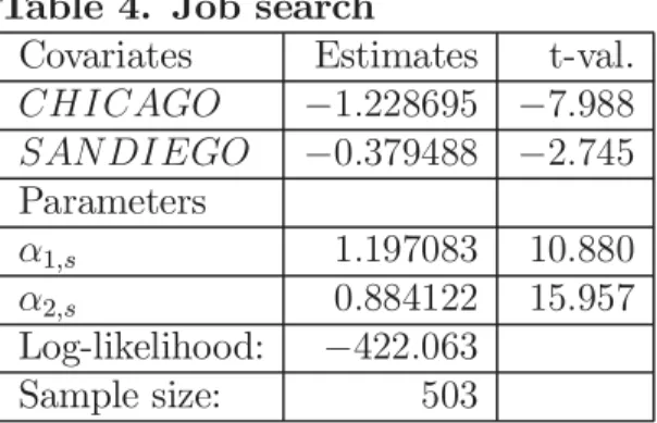
The estimation results for this model are presented in Table 4.

Table 4. Job search

Covariates Estimates t-val. CHICAGO −1.228695 −7.988

SANDIEGO ₋0.379488 ₋2.745

Parameters

α1,s 1.197083 10.880

α2,s 0.884122 15.957

Log-likelihood: −422.063

Sample size: 503

The results in Table 4 are only final with respect to the model specifi ca-tion. The coefficients involved will be re-estimated jointly with those of the recidivism model specified below. At that point we will interpret the results.

5.3 Recidivism of the control group

(19)

is independent of the job search duration Ts. Moreover, similar to the job

search case, the conditional survival function of Tc for the control group will

be modeled as a proportional hazard model:

Sc(t|X) = exp (₋exp (β_c0X)Λc(t)),

whereΛc(t)is the integrated hazard. Again, we may without loss of generality

assume that Λc(t)is piecewise linear, as in (9).

We have followed the same speciﬁcation strategy as for job search. The details can be found in the Appendix. Surprisingly, we ﬁnd that none of the covariates matter for recidivism, and that the baseline hazard is constant. Thus, the distribution of Tc for the control group is exponential, so that the

survival function involved takes the form

Sc(t|X) = exp (−αc.t). (11)

The maximum likelihood estimation result for αc is presented in Table 5:

Table 5. Recidivism (G= 0)

Parameter Estimate t-val.

αc 0.043681 7.396

Sample size: 134

Note that this result implies thatE[Tc|G= 0] = 1/αc ≈23 months, and

that approximately,

P (Tc ∈(0,1]|G= 0) ≈ 0.04274

P (Tc ∈(1,6]|G= 0) ≈ 0.18781

P (Tc ∈(6,12]|G= 0) ≈ 0.17740

P (Tc >12|G= 0) ≈ 0.59205

5.4 Incorporating conditional treatment

For the treatment group (G = 1), treatment is only received if Tc > Ts.

Therefore we will assume that if Tc ≤ Ts the distribution of Tc is the same

as for the control group:

(20)

See (11). This is the ”no anticipation” condition in Abbring and Van den Berg (2003, Assumption 1). Admittedly, in view of the eﬀect of group as-signment on attrition this may be a strong assumption. However, it follows from Table 2 that the number of individuals in the treatment group for which Tc ≤ Ts is relatively small, hence if this assumption is incorrect its impact

on the results will be minor.

Recall from the results of the preliminary data analysis that if there is a treatment eﬀect then it will likely work via the covariates. Therefore, let

P[Tc ≤t|Ts, Xc, G= 1] = 1−exp (−αc.Ts)

×exp (−αc.exp (βc0Xc).(t−Ts)) ift > Ts,

whereXc is the vector of covariates involved, which now also includes1for

the constant term. Thus, the conditional survival function ofTc givenTs, Xc,

and G is speciﬁed as

Sc(t|Ts, Xc, G) =P [Tc > t|Ts, Xc, G] =I(t≤Ts) exp (−αc.t) (12) +I(t > Ts) exp (₋αc.Ts).exp (−αc.exp (G.βc0Xc).(t−Ts)),

where I(.) is the indicator function.5

Note that the corresponding conditional hazard takes the form (8):

θc(t|Ts, X, G) = −

∂Sc(t|Ts, Xc, G)/∂t

Sc(t|Ts, Xc, G)

= αc(1 +I(t > Ts) (exp (G.β0cXc)−1)),

where the systematic hazardexp (β0

cXc)is now equal to1, the baseline hazard

λc(t) is equal to the constantαc,and

δ(t|Ts, X, G) = 1 +I(t > Ts) (exp (G.βc0Xc)−1).

Next, rewrite the survival function of Ts as

Ss(t|X) = exp (−exp (β_s0Xs)tαs), (13)

where now Xs = (CHICAGO, SANDIEGO,1)0 and αs = α2,s. See Table

(21)

4. Then it follows from (12) and (13) that for 0_≤a < b_≤p < q,

P[Tc ∈(p, q], Ts∈(a, b]|X, G]

= Z b

a

Sc(t|ts, Xc, G)d(−Ss(ts|Xs))

=₋

Z b

a

exp (₋αc.(1−exp (G.βc0Xc))ts)d(exp (−exp (βs0Xs)tαss ))

×(exp (−αc.exp (G.βc0Xc).p)−exp (−αc.exp (G.βc0Xc).q))

=

Z Ss(a|Xs)

Ss(b|Xs)

exp£−αc.exp

¡

−α−_s1β0_sXs ¢

×(1₋exp (G.β0

cXc)) (ln (1/u))1/αs

i

du

×(exp (₋αc.exp (G.βc0Xc).p)−exp (−αc.exp (G.βc0Xc).q)).

The parameters involved can now be (re-)estimated by maximum likelihood.6

Note that if there is a treatment eﬀect then the eﬀect is positive, in the sense that treatment reduces the risk of recidivism, if fort > Ts,

P[Tc > t|Ts, Xc, G= 1] > P[Tc > t|Ts, Xc, G= 0],

which is the case ifβ0

cXc <0.

5.5 Joint maximum likelihood results

In ﬁrst instance we have chosen for Xs in (12) the vector of all available

covariates, including 1 for the constant term. Again, we have conducted a series of Wald and likelihood ration test to remove insigniﬁcant covariates. See the Appendix for the details. The result (see Table 6) is that only two covariates matter for treatment: Age and the location dummy Boston. Note that the estimation results for job search are very close to the cor-responding estimates in Table 4, as expected. Moreover, observe that the estimate of αc in Table 6 is close to the estimate of αc in Table 5.

The signiﬁcant negative signs of the location dummies in the left-side panel of Table 6 indicate that the job search takes longer in Chicago and San Diego than in Boston, and in Chicago longer than in San Diego. Thus, its

6_{This has been done via the user-de}_ﬁ_{ned maximum likelihood module in} _EasyReg

(22)

Table 6. Job search, recidivism and treatment eﬀects

Job search

αs 0.875049 12.320

Covariates Estimates t-val. CHICAGO ₋1.225155 ₋7.440

SANDIEGO −0.324369 −2.141

1 0.184070 1.868

Recidivism

αc 0.041905 7.664

Covariates Estimates t-val. BOST ON 0.425046 2.304

AGE −0.045503 −2.720

1 1.222241 2.536

Log-Likelihood: ₋847.358

Sample size: 503

seems that the ex-convicts in Boston receive more or better help with the job search than in the other two cities. Other possible reasons for these effects are differences in labor market conditions, efficiency of programs, attitudes of employers regarding ex-convicts, and policies regarding the release of criminal records information, to mention a few. However, we do not have enough data information to pinpoint the reasons for the differences in job search durations in these three locations.

(23)

5.6 Treatment e

ﬀ

ects

It is straightforward to verify from (12) that

P[Tc ≤t|Tc > Ts, Ts, Xc, G]

= 1₋exp (₋αc.exp (G.βc0Xc).(t−Ts))I(t > Ts)

hence

E[Tc|Tc > Ts, Ts, Xc, G] = Ts+α−c1exp (−G.βc0Xc)

and thus

E[Tc|Tc > Ts, Ts, Xc, G= 1]−E[Tc|Tc > Ts, Ts, Xc, G= 0] (14)

= α_c−1(exp (₋β_c0Xc)₋1).

This expression may be interpreted as (a version of) the conditional ment eﬀect. Thus, the treatment has a positive eﬀect, in the sense that treat-ment increases the expected time between release and rearrest, if β0

cXc <0,

regardless the job search duration.

It follows from the results in Table 6 that

b

β0_cXc = 1.222241 + 0.425046.BOST ON −0.045503.AGE. (15)

As to the ”Boston” effect, (15) is larger for Boston than for the other two lo-cations, so that ceteris paribus the conditional treatment effect on recidivism in Boston is less than in Chicago and San Diego. This difference increases with age. Moreover, it follows from (15) the treatment reduces the risk of recidivism in Chicago and San Diego if

AGE > 1.222241

0.045503 ≈27, (16)

and in Boston if

AGE > 2.180753

0.045503 ≈36.

(24)

Figure 1: Conditional treatment eﬀect on recidivism

5.7 Comparison with the preliminary data analysis

In the preliminary data analysis we have argued that if the dependence of P [Tc ≤t|Ts, Xc] on Ts is substantially reduced after Xc is integrated out,

then the inequality (3) is no longer detectable. To verify this conjecture, we have estimated P [Tc ∈(p, q]|Ts =ts, Xc, G = 1]for ts < p on the basis of

the results in Table 6 and then averaged these estimates over the treatment group, which yield the results in Table 7.

Table 7. EstimatedP [Tc ∈(p, q]|Ts =ts, G= 1]

p q Range ofts Mean Minimum Maximum

1 6 0→1 0.20697 0.20567 0.20829

6 12 0_→1 0.18507 0.18405 0.18610

6 12 1_→6 0.19164 0.18610 0.19753

12 _∞ 0_→1 0.56324 0.56194 0.56457

12 ∞ 1→6 0.57202 0.56457 0.58015

12 _∞ 6_→12 0.59190 0.58015 0.60480

Indeed, the dependence ofP[Tc ∈(p, q]|Ts=ts, G= 1]onts < pis weak,

(25)

6 Conclusions

In contrast with previous studies we find that the ESEO program has an effect on recidivism, but this effect depends on age and location: the ESEO program reduces the risk of recidivism only for ex-inmates over the age of 27 in San Diego and Chicago, and over the age of 36 in Boston, but increases the risk of recidivism for the other ex-inmates in the treatment group. However, in view of Figure 1 it seems that the positive effect of the treatment for the older ex-convicts outweighs the negative effect for the younger ex-convicts, in terms of the expected number of months with which the rearrest will be postponed. Hence, heterogeneity of impact is an important point to consider when evaluating reentry programs.

One of the agreements in the literature on program evaluation is that given the specificities of the groups of people who usually make use of those services, some programs that work well for a given group may not work so well for others. In other words, the effects of programs may be heterogenous. See, for example, Heckman et al. (1999). That is exactly what we find.

Our results provide evidence that employment programs for ex-offenders can reduce recidivism, provided that these programs take the heterogeneity of the population of ex-offenders into account. A program that is uniform for all ex-offenders may not yield the expected results. This paper has therefore made a positive contribution to the debate in the criminological literature about the likely effects of ex-offenders employment programs. See Visher et al. (2005).

In unemployment duration studies, age and education are usually im-portant factors for the length of the unemployment spell. In the case under review, however, the job search duration does not depend on any individual-specific covariates. This may be due to the fact that all individuals in the sample have one dominant characteristic in common, namely being ex-convicts. Moreover, ourfinding that the job search duration only depends on the location may also indicate that this duration mainly measures the efforts of the program staff in the three locations infinding jobs for the ex-inmates, rather than the efforts of the ex-inmates themselves.

(26)

and employment history, the status of their release (parole, probation, or un-conditional release), time served versus sentence time, family characteristics, level of participation in the job search, the types of jobs searched for, and past and presents employer’s evaluations. Moreover, we fail to understand the reason why in the ESEO data the job search and recidivism durations were interval censored. If we had observed uncensored durations, we would have been able to conduct a more sophisticated econometric analysis, for ex-ample by including unobserved heterogeneity in our model. Finally, future program evaluations should pay more attention to the attrition problem, in particular by trying to trace down the drop-outs and gathering information about the reasons for dropping out.

7 Appendix

7.1 Attrition

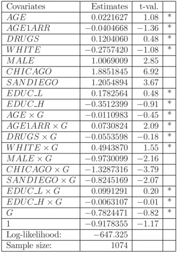
The initial Logit results for attrition are presented in Table A.1.

The parameters in Table A.1 indicated by an asterix (*) are individu-ally insignificant at the 5% significance level. The Wald test that they are also jointly zero does not reject the null hypothesis at any conventional sig-nificance level. Therefore, we have re-estimated the model without these covariates. The results are presented in Table A.2.

The likelihood-ratio (LR) test that the model in Table A.1 can be reduced to the model in Table A.2 has p-value 0.32867. Therefore, the null hypoth-esis involved cannot be rejected. The Wald test of the hypothhypoth-esis that the parameters of M ALE andM ALE ×G add up to zero has p-value0.55700, hence we may replace these two covariates with MALE×(1₋G) only, with approximately the same coefficient as MALE in Table A.2. Thus, males have a higher attrition rate than females, ceteris paribus, but only if selected in the control group. The Wald test of the hypothesis that the coefficients of CHICAGO and CHICAGO×Gadd up to zero has p-value0.01127, hence this hypothesis should be rejected. The same applies to the hypothesis that the coefficients of SAN DIEGO and SANDIEGO×Gadd up to zero: The p-value of the Wald test involved is 0.04173.

(27)

Table A.1. Initial Logit results for attrition

AGE 0.0221627 1.08 *

AGE1ARR ₋0.0404668 ₋1.36 *

DRUGS 0.1204060 0.48 * W HIT E −0.2757420 −1.08 *

MALE 1.0069009 2.85

CHICAGO 1.8851845 6.92

SANDIEGO 1.2054894 3.67

EDUC L 0.1782564 0.48 * EDUC H −0.3512399 −0.91 *

AGE×G ₋0.0110983 ₋0.45 *

AGE1ARR×G 0.0730824 2.09 *

DRUGS×G −0.0553598 −0.18 * W HIT E×G 0.4943870 1.55 *

MALE×G ₋0.9730099 ₋2.16

CHICAGO×G −1.3287316 −3.79

SANDIEGO×G −0.8245169 −2.07

EDUC L×G 0.0991291 0.20 * EDUC H×G ₋0.0063107 ₋0.01 *

G −0.7824471 −0.82 *

1 ₋0.9178355 ₋1.17

Sample size: 1074

Table A.2. Logit results for attrition: Model 2

MALE 0.8708543 3.51

MALE×G ₋0.7345117 ₋3.41

CHICAGO 1.8323490 7.84

CHICAGO×G ₋1.3317171 ₋4.58

SAN DIEGO 1.0773423 3.59

SAN DIEGO×G ₋0.6531673 ₋1.88

1 ₋0.8711105 ₋3.78

Log-likelihood: −654.658

(28)

7.2 Preliminary data analysis

To test whether

P [Tc ∈(1,6]] =P [Tc ∈(1,6]|Ts ∈(0,1]] (17)

P [Tc ∈(6,12]] =P[Tc ∈(6,12]|Ts∈(0,1], Ts ∈(1,6]] (18)

P [Tc ∈(12,∞)] (19)

=P[Tc ∈(12,∞)|Ts ∈(0,1], Ts ∈(1,6], Ts∈(6,12]]

we have estimated Logit models for each of these conditional probabilities, and for each group separately:

P[Tc ∈(1,6]|Ts ∈(0,1]] =F (β1,0+β1,1I(Ts∈(0,1]) +β1,2) (20)

P[Tc ∈(6,12]|Ts ∈(0,1], Ts ∈(1,6]] (21)

=F(β2,0+β2,1I(Ts∈(0,1]) +β2,2I(Ts ∈(1,6]))

P[Tc ∈(12,∞)|Ts ∈(0,1], Ts ∈(1,6], Ts ∈(6,12]] (22)

=F(β3,0+β3,1I(Ts∈(0,1]) +β3,2I(Ts ∈(1,6]) +β3,3I(Ts ∈(6,12]))

where F(x)is the logistic distribution function. However, in the case G= 0

we have I(Ts∈(0,1]) +I(Ts ∈(1,6]) +I(Ts ∈(6,12]) = 1, so that in the

case (22) we can only estimate

P [Tc ∈(12,∞)|Ts∈(0,1], Ts ∈(1,6]]

=F (β3,0+β3,1I(Ts ∈(0,1]) +β3,2I(Ts ∈(1,6])) (23)

(29)

Table A.3. Logit results for (20)-(22)/(23) Treatment group (G= 1)

i βi,0 βi,1 βi,2 βi,3 Wald test

(t-value) (t-value) (t-value) (t-value) (p-value)

1 −1.2809338 −0.0391111 0.0225

(₋7.17) (₋0.15) (0.88076)

2 ₋1.5040774 ₋0.0606246 0.1094842 0.88076

(−3.33) (−0.12) (0.22) (0.83261)

3 0.4054651 ₋0.1335314 ₋0.2595112 0.1823216 1.19

(0.44) (₋0.14) (₋0.28) (0.18) (0.75601)

Table A.4 . Logit results for (20)-(22)/(23) Control group(G= 0)

i βi,0 βi,1 βi,2 Wald test

(t-value) (t-value) (t-value) (p-value)

1 ₋1.2992830 0.0216225 0.0025

(₋3.99) (0.05) (0.96012)

2 −1.6094379 −0.1973594 0.0930904 0.35

(₋1.47) (₋0.17) (0.08) (0.83801)

3 ₋0.6931472 1.1093076 1.1826954 1.69

(30)

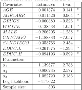
Table A.5. Job search: Model 1

AGE 0.001374 0.141 *

AGE1ARR 0.011526 0.964 *

DRUGS −0.060380 −0.526 * W HIT E 0.128538 1.051 *

MALE −0.206205 −1.258 *

CHICAGO ₋1.188883 ₋7.057

SANDIEGO ₋0.353766 ₋2.454

EDU C L −0.261975 −1.393 * EDU C H ₋0.094193 ₋0.592 * Parameters

α1 1.139577 2.788

α2 0.806235 2.577

α3 1.082720 2.186

Sample size: 503

7.3 Job search model speci

ﬁ

cation

The initial maximum likelihood results for job search are presented in Table A.5. Recall that theα’s are the parameters of the integrated baseline hazard (9).

The Wald test of the hypothesis that the coefficients of the covariates in Table A.5 indicated by an asterix (*) are jointly zero has p-value 0.45137. The Wald test of the null hypothesis α1 = α2 = α3 has p-value 0.10356, so that the null hypothesis involved cannot be rejected at the 10% significance level. Recall that the latter hypothesis implies that the baseline hazard is constant. However, for the time being we will not implement the restriction α1 = α2 = α3. First, we will get rid of the insignificant covariates. The results are presented in Table A.6.

(31)

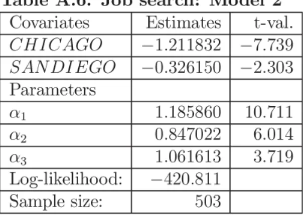
Table A.6. Job search: Model 2

SANDIEGO ₋0.326150 ₋2.303

Parameters

α1 1.185860 10.711

α2 0.847022 6.014

α3 1.061613 3.719

Sample size: 503

As a double-check whether the model can be reduced from the initial model in Table A.5 to the model in Table 4 we have conducted the likelihood-ratio test: The LR test involved has p-value 0.35230, hence the hypothesis cannot be rejected at any conventional signiﬁcance level. Moreover, the t-test statistic of the null hypothesis α2,s = 1 has value−2.091,which is borderline

significant at the 5% level for the two-sided t-test, and significant for the left-sided t-test (the corresponding left-sided p-value is 0.01826). Since it is implausible that the ”hazard” of finding a job increases with the job search duration, the left-sided result prevails.

7.4 Recidivism of the control group

The initial maximum likelihood results are presented in Table A.7.

The covariateAGE is borderline significant at the 5% level; all the other covariates are insignificant at any conventional significance level. The Wald test that all the coefficients of the covariates (including the one for AGE) are zero has p-value 0.32881, hence the null hypothesis that Tc does not

depend on covariates cannot be rejected at any conventional signiﬁcance level. Moreover, the Wald test of the null hypothesis α1 = α2 = α3 has p-value

0.80083, and therefore cannot be rejected at any conventional signiﬁcance

level. Recall that this hypothesis is equivalent to the hypothesis thatΛc(t) =

α1t.Thus, the distribution ofTc for the control group is exponential, without

covariates!

(32)

Table A.7. Recidivism of the control group: Initial model

AGE ₋0.057819 ₋2.098

AGE1ARR −0.061837 −1.716

DRUGS 0.232762 0.733

W HIT E ₋0.012282 ₋0.036

M ALE −0.290917 −0.721

CHICAGO 0.287844 0.725

SANDIEGO 0.069299 0.165

EDUC L ₋0.103330 ₋0.206

EDUC H 0.748567 1.741

Parameters:

α1 0.366003 0.906

α2 0.609465 0.957

α3 0.493359 1.010

Sample size: 134

exponential model (11) for the recidivism of the control group.

7.5 Joint maximum likelihood results

The initial maximum likelihood estimation results are presented in Table A.8, for recidivism only.

The parameters in Table A.8 indicated by an asterix (*) are jointly in-signiﬁcant: The p-value of the Wald test involved is 0.42136. Therefore, in the next estimation round these covariates have been removed. See Table A.9.

The Wald test that only AGE matters for recidivism yields p-value

0.03464, hence this hypothesis is rejected at the 5% signiﬁcance level. The

(33)

Table A.8. Recidivism: Model 1

Covariates Estimates t-val. DRU GS −0.217296 −1.027 * CHICAGO ₋0.523601 ₋2.073

SANDIEGO ₋0.461512 ₋1.926

W HIT E −0.278290 −1.332 *

MALE ₋0.050078 ₋0.154 *

EDUC L 0.576838 1.874

EDUC H ₋0.330336 ₋0.939 *

AGE −0.040221 −2.200

AGE1ARR −0.030686 −1.292 *

1 2.245037 3.226

αc 0.041529 7.672

Log-Likelihood: ₋842.896

Sample size: 503

Table A.9. Recidivism: Model 2

SANDIEGO ₋0.460476 ₋2.030

EDUC L 0.487441 1.639

AGE −0.047794 −2.870

1 1.707907 3.581

αc 0.040407 7.550

Log-Likelihood: −845.992

(34)

dummies replaced by the dummy variable BOST ON. See Table 6.

As a double-check we have conducted the LR test that the initial model in Table A.8 can be reduced to the model in Table 6. The p-value of the test

is 0.25816.

References

Abbring JH, Van den Berg GJ (2003): The non-parametric identiﬁcation of treatment eﬀects in duration models, Econometrica, 71, 1491-1517.

Abbring JH, Van den Berg GJ, Van Ours JC (2005): The eﬀect of un-employment insurance sanctions on the transition rate from unun-employment to employment, Economic Journal, 115, 602-630.

Bierens HJ (2006): EasyReg International, Pennsylvania State Univer-sity. http://econ.la.psu.edu/~hbierens/EASYREG.HTM.

Bierens HJ (2007): Semi-nonparametric interval-censored mixed propor-tional hazard models: Identiﬁcation and consistency results, Econometric Theory, forthcoming. http://econ.la.psu.edu/~hbierens/SNPMPHM.PDF.

Bierens HJ, Carvalho JR (2007): Semi-nonparametric competing risks analysis of recidivism,Journal of Applied Econometrics,22, 971-993. http:// econ.la.psu.edu/~hbierens/RECIDIVISM2.PDF.

Bloom HS (1984): Accounting for no-shows in experimental evaluation design, Evaluation Review, 8, 225-246.

Bloom D (2006): Employment-focused programs for ex-prisoners. What have we learned, what are we learning, and where should we go from here? Michigan Disability Rights Coalition. http://www.mdrc.org/publications /435/full.pdf.

Bureau of Justice Statistics (1994): Recidivism of Prisoners Released in 1994.

Beck AJ, Shipley BE (1989): Recidivism of prisoners released in 1983, Special report, Bureau of Justice Statistics.

Carvalho JR, Bierens HJ (2007): Conditional treatment and its eﬀect on recidivism, Brazilian Review of Econometrics, 27, 53-84. http://econ.la.psu .edu/~hbierens/CONDTREAT.PDF.

Devine T, Kiefer N (1991): Empirical Labor Economics: The Search Approach. Oxford University Press, New York.

(35)

women: Evidence from experimental data, Review of Economic Studies, 64, 655 682.

Fagan J, Freeman R (1999): Crime and work, Crime and Justice, 25, 225-290.

Farrington DP, Welsh BC (2005): Randomized experiments in criminol-ogy: what have we learned in the last two decades? Journal of Experimental Criminology, 1, 9-38.

Freeman R (1999): Economics of crime. The Handbook of Labor Eco-nomics, Vol 3C, North Holland, Amsterdam.

Freeman R (2003): Can we close the revolving door?: Recidivism versus employment of ex-oﬀenders in the US.,Urban Institute Reentry Round Table, New York University Law School.

Gendreau P, Little T, Goggin C (1996): A meta-analysis of the predictors of adult oﬀender recidivism: What works!, Criminology, 34, 575 607.

Harer MD (1994): Recidivism among federal prisoners released in 1987, Journal of Correctional Education, 46, 98-127.

Heckman J, Lalonde RJ, Smith JA (1999): The economics and econo-metrics of active labor market programs,Handbook of Labor Economics, Vol. 3A, Elsevier Science, Amsterdam, 1865-2097.

Heckman J, Smith J, Taber C (1998): Accounting for dropouts in evalu-ations of social programs, The Review of Economics and Statistics, 80, 1-14. Maltz MD (1984): Recidivism: Quantitative Studies in Social Sciences. Academic Press, Orlando, FL.

Milkman R (2001): Employment services for ex-oﬀenders, 1981-1984: Boston, Chicago, and San Diego, Discussion Paper 8619, ICPSR.

Milkman R, Timrots A, Peyser A, Toborg M, Yezer BGA., Carpenter L, Landson N (1985): Employment services for ex-oﬀendersﬁeld test, Discussion paper, The Lazar Institute.

Pissarides CA (2000): Equilibrium Unemployment Theory (Second edi-tion). MIT Press, Cambridge, MA.

Sampson RJ, Laub JH (1997): A life-course theory of cumulative disad-vantage and the stability of delinquency, Advances in Criminological The-ory,7, 133-161.

Seiter RP, Kadela KR (2003): Prisoner reentry: what works, what does not, and what is promising, Crime & Delinquency, 49,360-388.

(36)

Timrots A (1985): An evaluation of employment services programs for ex-oﬀenders, Masters thesis, University of Maryland, College Park.

Uggen C (2000): Work as a turning point in the life course of criminals: A duration model of age, employment and recidivism,American Sociological Review, 65, 529-546.

Van den Berg GJ (1999): Empirical inference with equilibrium search models of the labor market, The Economic Journal, 109, 283-306.

Van den Berg GJ (2000): Duration models: Speciﬁcation, identiﬁcation, and multiple durations, Handbook of Econometrics, Vol. V, North Holland, Amsterdam.

Van den Berg GJ, Van der Klaauw B, Van Ours JC (2004): Punitive sanctions and the transition rate from welfare to work, Journal of Labor Economics, 22, 211-241.

Visher CA, Winterﬁeld L, Coggeshall MB (2005): Ex-oﬀender employ-ment programs and recidivism: a meta-analysis, Journal of Experimental Criminology, 1, 295-316.