Alexandre Bragança Coelho Danilo Rolim Dias de Aguiar James S. Eales
Resumo
O objetivo deste artigo é analisar a demanda de alimentos no Brasil por meio da estimação de um sistema de demanda com dezoito produtos usando dados da Pesquisa de Orçamentos Familiares realizada em 2002 e 2003 (POF 2002/2003). A forma funcional utilizada foi o Quadratic Almost Ideal Demand System (QUAIDS). A estimação utiliza o Procedimento de Shonkwiler e Yen para lidar com o problema do consumo zero. Os resultados mostraram que as probabilidades de aquisição dos produtos básicos foram negati-vamente relacionadas com a renda familiar mensal, enquanto carnes, leite e outros produtos mostraram uma relação positiva. As variáveis de educação, regionais e de localização do domicílio também foram importantes no primeiro estágio da estimação. Em relação às elasticidades-renda, nenhum bem foi con-siderado inferior e seis de dezoito foram concon-siderados bens de luxo.
Palavras-Chave
Demanda de alimentos, Modelo QUAIDS, Procedimento de Shonkwiler e Yen
Abstract
The objective of the analysis is to estimate a demand system including eighteen food products using data from a Brazilian Household Budget Survey carried out in 2002 and 2003 (POF 2002/2003). The functional form used was Quadratic Almost Ideal Demand System (QUAIDS). Estimation employs the Shonkwiler and Yen method to account for zero consumption. Results showed that purchase probabilities of staples foods were negatively related to family monthly income, while meat, milk and other products showed a positive relation. Regional, educational and urbanization variables were also important in the first stage estimation. While some of the goods had negative income coefficients, none were inferior and six of eighteen were luxuries based on second stage estimates.
Keywords
Brazilian Food Demand, QUAIDS Model, Shonkwiler & Yen method
JEL Classiication D12, C25, R22
Universidade Federal de Viçosa (UFV). Endereço para contato: Campus da Universidade Federal de
Viço-sa, s/n. Departamento de Economia Rural - Viçosa - MG. CEP: 36571-000. E-mail: [email protected].
Universidade Federal de São Carlos (UFSCar), Campus de Sorocaba. E-mail: [email protected].
Purdue University (USA).E-mail: [email protected].
1 Introduction
Food demand in Brazil has undergone major changes in the last few decades caused by structural shifts such as urbanization, changes in demographic characteristics and increase in women’s participation in the labor force. Therefore, it is necessary to identify families’ new consumption patterns thoroughly in order to support both the design of appropriate government policies and the implementation of business strategies.
In order to devise proper public policies, understanding of food demand patterns is crucial (BaTalha et al., 2005). In Brazil, income redistribution and food secu-rity programs have been implemented aiming to reduce income inequality, hunger, and poverty. In order to be implemented correctly, these programs must take into consideration how changes in income would affect food consumption.
Other kinds of government policies depending on demand information are product support and inflation control programs. In the case of support programs, the gov-ernment needs to know how the consumption of a product has changed through time to devise policies to prevent supply shortages. For instance, previous studies (see hOFFmann, 1995) have shown a decrease in home consumption of rice and beans and an increase in consumption of some fruits, vegetables and beef. Such trends should be considered as the government designs its support programs. Regarding inflation control, the percentage of household income spent on food has decreased in recent decades, but is still the second most important in families’ ex-penses with an average share of 21% (Instituto Brasileiro de Geografia e Estatística (IBGE, 2004b). Furthermore, food purchases are still the most important expense for low income families, mainly in Brazil’s north and northeast areas. according to the 2002/2003 Brazilian household Budget Survey (Pesquisa de Orçamentos Familiares (POF) 2002/2003), low income Brazilian families spend 33% of their income on food. These households suffer the most when food prices increase, so policymakers must have good estimates of price elasticities as inflation control programs are designed. Finally, in terms of business strategies, information on con-sumption patterns is crucial to investment planning and to design marketing and product development programs.
In sum, demand function parameters provide useful information to the government, farmers and the private sector. Despite some previous studies of food demand in Brazil,1
this paper main contribution is to deal with the zero expenditure problem
1 See, for example, Bacchi (1989), Furtuoso (1981), Thomas et al (1991) for early studies and aguero
and Gould (2003), menezes, Silveira e azzoni (2005), Silveira et al. (2007a) and Silveira et al.
usually present whenever large household consumption data are used and which is commonly overlooked in empirical applications. Therefore, the objective of the current effort is to fill this gap. This will be accomplished through the estimation of a food demand system comprised of 18 Brazilian food products. Besides price and income effects, the system will account for regional differences among food demand patterns, as well as differences between urban and rural areas and other household demographics.
2 Data
The data used in this analysis were obtained from the 2002/2003 Brazilian household Budget Survey microdata2 (POF 2002/2003) carried out by the Brazilian
Institute of Geography and Statistics (IBGE). This survey contains one week de-tailed diary of food purchases for at-home consumption by Brazilian households. The 2002/2003 survey is different from previous surveys for two main reasons: First, it covered the entire Brazilian territory, including rural areas, whereas pre-vious surveys examined only urban consumption. Second, for the first time non-monetary purchases3 were considered, which are very important in rural areas.
Eighteen food products were selected for study from POF’s wide range of products according to their importance in consumers’ food budget and the substitutability among them. The selected food products are: sugar, rice, bananas, potatoes, prime cut beef, low quality beef, manioc flour, beans, chicken, powdered milk, fluid milk, pas-ta, butter, margarine, French rolls, pork, cheese and tomatoes.4 Prices were obtained
using unit values calculated from the microdata. missing prices were replaced by average state prices.5 The sample size used in the estimation is 43,922 households.
3 Methodology
The use of household Budget Survey microdata allows a specification of demand equations that capture heterogeneity among consumers. In consumer demand mod-eling, detailed demographic information allows treatment of exogenous preferences which is not possible with aggregate time series (YEn; Kan; SU, 2002). This usually represents a better description of different groups demand patterns and a
2 See IBGE (op. cit, 2004b).
3 according to IBGE (2004a), non-monetary purchases comprise everything that is produced,
fished, hunted, collected or received in goods utilized or consumed during the survey and, at least in the last transaction, have not gone through a market.
4 See appendix a3 for statistics on average expenditures.
great adherence of models to reality (BlUnDEll; PaShaRDES; WEBER, 1993; manChESTER, 1977). however, when microdata are used, the problem of zero expenditure often appears, that is, people often appear in these surveys consuming zero of different products. The causes are twofold: the infrequency of purchases, caused by the relatively short period of data collection and a corner solution to the consumer maximization problem. This represents a major estimation problem, since there is a censored dependent variable. This problem is particularly complicated in multivariate models such as demand systems (YEn; Kan; SU, op. cit.).
In this case, ordinary least squares estimates (OlS) are known to be biased and in-consistent (GREEnE, 2000). In individual demands, maximum likelihood (ml) es-timation of Tobit models may be performed. however, as far as demand systems are concerned, direct ml estimation of these models remains difficult when censoring occurs in multiple equations because of the need of evaluating multiple integrals in the likelihood functions (ShOnKWIlER; YEn, 1999). Besides, one stage models as Tobit assume that there is simultaneity between the purchase decision and the quan-tity decision. haines, Guilkey, and Popkin (1988) argue that the food consumption decision should be modeled as a two-stage problem: not only these decision stages are different, but the variables concerning each stage may differ as well.
These issues stimulated the use of two-step estimation procedures with limited dependent variables to model food system demand estimation (hEIEn; WESSElS, 1990; ShOnKWIlER; YEn, op. cit.). These procedures allowed dealing with the zero consumption problem, were simpler than the direct ml estimation (lEE; PIT, 1986) and did not presented aggregation problems, since microdata could be readily used. as the heien and Wessels procedure presented inconsistencies and performed poorly in monte Carlo simulations,6 Shonkwiler and Yen (op. cit.)
two-step estimation will be used in this paper.
Suppose initially that we wish to model the demand of m food products and there are n households in the dataset. Shonkwiler and Yen approach this problem as a two-step estimation:
First step
* '
in in i in
d =Z α + υ
*
*
1 if
0
0 if
0
in
in
in
d
d
d
>
=
≤
for all i=1,...,M & n=1,...,N (1)
second step
*
( , )
in in i in
y = f X β +e (2)
* in in
in
d
y
y
=
for alli
=
1
,...,
M
&n
=
1
,...,
N
where
*
in
d = Unobserved variable representing the utility difference when the consumer
buys or does not buy the ith food product;
in
d =Observed dichotomous variable representing whether the consumer buys
(
d
in=
1
) or does not buy (d
in=
0
) the ith food product;in
Z = Vector of exogenous variables which affects the purchase decision;
i
α = Parameter vector in the purchase decision equation;
in
y =Observed dependent variable representing the consumed quantity of the ith
food product;
(
in,
i)
f X
β =
Functional form of the demand function;in
X = Vector of exogenous variables which impact the quantity decision;
i
β =Parameter vector in the quantity decision equation;
in
υ & ein= random errors.
Shonkwiler and Yen (op. cit.) argue that this system can be estimated by means of a two-step procedure using all observations, no matter the purchase decision. In the first step, known as the purchase decision, probit estimates, αˆi, of αi are
ob-tained and then they are used in the second step to calculate ϕ(Zin'αˆi) & Φ(Zin'αˆi)
and estimate the parameters βi & δi in the system:
ˆ ˆ
( ' ) ( , ) ( ' )
in in i in i i in i in
y = Φ Z α f X β + δ ϕ Z α + η (3)
(i=1,...,M &
n
=
1
,...,
N
)where ϕ(Zin'αi) is the normal probability density function (pdf) evaluated at
'
in i
Z α , Φ(Zin'αi)is the normal cumulative density function (cdf) evaluated atZin'αi
The equation system represented in (3) is estimated by maximum likelihood with a non-linear Seemingly unrelated regression (SUR). To implement the Shonkwiler and Yen estimation procedure, it is necessary to specify the demands’ functional form
f X
(
in,
β
i)
. The Quadratic Almost Ideal Demand System (QUaIDS) isem-ployed, below. The QUaIDS model has more flexibility than the well known Almost Ideal Demand System (aIDS), allowing for non-linear Engel curves but maintaining all the relevant properties of its linear counterpart.7 It relates the ex-penditure share of each good to the usual explanatory variables (price and income), and to variables that capture consumers’ heterogeneity. Substituting the QUaIDS functional form into equation (3), the system to be estimated becomes:
2
1 1
ˆ ˆ
( ' )( ln ln ln ) ( ' )
( ) ( ) ( )
n n
i
in in i ik k ij j i i in i in
k j
m m
w Z V p Z
a p b p a p
= =
λ
= Φ α θ + γ + β + + δ φ α + η
∑
∑
(4)(i=1,...,M & n=1,...,N)
where in in in
p q
w
m
=
=
ith food product expenditure share for consumer n;=
k
V
Demographic variables;j
p =Price of good i;
i
q =Quantity of good i;
=
m
monthly household income0
ln ( ) ln
n
j j j=1
a p =
∑
w p.
0
j
w =mean shares.
k k
b(p)=
∏
pβλ.
, , , ,
i i i ij i
θ β δ γ λ =Parameters.
With Shonkwiler and Yen estimation ensuring adding up is a problem. The usual parameters restriction method only guarantees adding up of the latent expenditure shares, but not observed expenditure shares (DOnG; GOUlD; KaISER, 2004). One solution to this problem8 is to treat one of the products as a “residual good”
and to estimate the system with (n-1) goods. Then, we have the nth equation as:
7 See Banks, Blundell and lewbel (1997)
1
1
1 ( , ) ( , )
n
n k in n k n in n n
k
w f X e f X e
−
=
= −
∑
β + = β + (5)where
( in, i)
f X β = Functional form of the demand function; 1
1
( , ) 1 ( , )
n
n in i k in n
k
f X f X
−
=
β = −
∑
β ;1
1
n
n k
k
e e
−
=
= −
∑
This method guarantees that the sum of the (n-1) estimated equations and the nth equation equals one. Then, the likelihood function is constructed only with the first (n-1) equations. The elasticities of the nth good can be calculated by the adding up restrictions.
There are some problems with this method. First, parameter estimates are not in-variant to the commodity chosen for omission. Second, there is no guarantee that estimated expenditure shares will be non-negative. nevertheless, this solution is used here as it was felt that problems caused by zero consumption were the most severe. The residual commodity generally chosen is the good that the researcher has the least interest.9 Sugar is excluded during estimation because its share of
consumers’ expenditure is small.
4 Results
4.1 First step Results
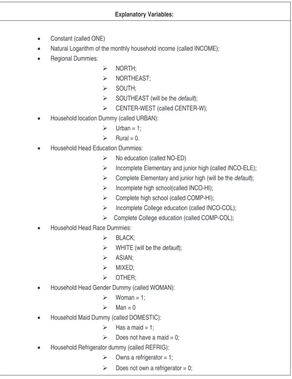
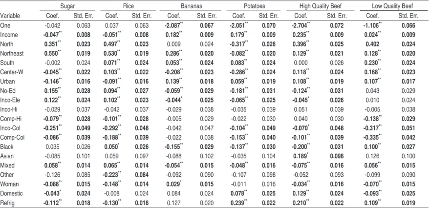
Shonkwiler and Yen first step estimation consists of estimating equations using the probit model for each food product. The dependent variable is a dichotomous variable which is 1 if the consumer purchases the product and zero otherwise. The explanatory variables we used are presented in Table 1:
9 Generally, the residual commodity is the category ‘other foods’, very common in demand studies.
Explanatory Variables:
• Constant (called ONE)
• Natural Logarithm of the monthly household income (called INCOME);
• Regional Dummies:
NORTH;
NORTHEAST;
SOUTH;
SOUTHEAST (will be the default);
CENTER-WEST (called CENTER-W);
• Household location Dummy (called URBAN):
Urban = 1;
Rural = 0.
• Household Head Education Dummies:
No education (called NO-ED)
Incomplete Elementary and junior high (called INCO-ELE);
Complete Elementary and junior high (will be the default);
Incomplete high school(called INCO-HI);
Complete high school (called COMP-HI);
Incomplete College education (called INCO-COL);
Complete College education (called COMP-COL);
• Household Head Race Dummies:
BLACK;
WHITE (will be the default);
ASIAN;
MIXED;
OTHER;
• Household Head Gender Dummy (called WOMAN):
Woman = 1;
Man = 0
• Household Maid Dummy (called DOMESTIC):
Has a maid = 1;
Does not have a maid = 0;
• Household Refrigerator dummy (called REFRIG):
Owns a refrigerator = 1;
Does not own a refrigerator = 0;
First step results are presented in table a1 in the appendix.10 a general inspection
reveals that 263 out of 360 coefficients are significant (73.06 %). Coefficient signs mostly correspond to expectations. For income, for example, an increase in house-hold income causes a decrease in the purchase probability of rice and sugar. For beans and manioc flour, income coefficients are also negative, but not statistically significant. For other products, an increase in household income causes an increase of the purchase probability.
For regional differences, most coefficients are significant, showing that there are specific regional differences in consumption in relation to the southeast region (default), even though we control for income differences. This is an important re-sult because it suggests that the purchase probabilities for some food products are influenced by regional factors (taste, existence of substitutes, etc.) and not only by the very sharp regional differences in income that exist in Brazil. For example, purchase probabilities for pork are much higher in the south than in the other regions of the country. accordingly, north and northeast11 variables have a posi-tive impact on purchase probabilities for some basic food products such as rice, beans and manioc flour. Some results were surprising, such as the positive coef-ficient for the northeast in the high quality beef equation, since the consumption of this product is much higher in the southeast region. One possible explanation is that, controlling for differences in income, household consumption is higher in the northeast area whereas high quality beef consumption away from home is higher in the southeast.
Only two of eighteen InCO-hI coefficients and eight of eighteen COmP-hI are significant. Thus, there is almost no difference in purchase probability between households whose head has a high school education (complete or not) and house-holds whose head completed only junior high or less. nevertheless, coefficients of other educational variables, such as nO-ED, InCO-COl, and COmP-COl are significant, for the most part, and the signs are almost all negative. When the household head has no education, positive coefficients result for sugar, rice, manioc flour, beans and low grade beef (not significant) and negative values for other prod-ucts. Demand for cheaper, high-energy foods, such as rice, sugar and manioc flour is higher for those who have to do manual labor, which is very common for those who have little or no education. Results for the college degree variables show nega-tive coefficients for all products with exception of cheese and butter (not signifi-cant), indicating smaller purchase probabilities than households whose head have
10 The software used was GaUSS 6.0 for Windows, Copyright 1984-2003, aptech Systems, Inc.
11 north and northeast regions are the poorest regions in Brazil, with health statistics comparable
completed only junior high. This result may stem from more educated households eating out more often than their less educated counterparts.
Results for urban-rural coefficients are significant for all products except chicken, pasta and pork. The signs are according to expectation, with negative values for cheaper, high-energy foods indicating a higher purchase probability in rural areas and positive signs for products such as French rolls, beef, cheese, powdered milk, meaning that their purchase probability is higher in urban areas.
Results for race variables show that 30 out of 72 coefficients are not significant, especially the coefficients from aSIan and OThERS variables. Thus, for most commodities, there is no significant difference between those households whose head is asian or from other race (except black, white, or mixed) and households whose head are white. The results for BlaCK and mIXED show a positive influ-ence in the purchase probability of sugar, rice, low quality beef, manioc flour and negative influence on fluid milk, high quality beef, bananas, potatoes, tomatoes, and cheese.
Results for influence of household head gender show that most coefficients are significant and negative; for example, for sugar, rice and beans. For milk, the coef-ficient is not significant and for cheese there is a significant and positive coefcoef-ficient. For bananas and French rolls, this variable has a positive influence on the purchase probability. It is hard to find a complete explanation for this behavior. The expec-tation was that women have greater concern with health issues than men and that WOman should have a positive effect on healthy foods (fruits, vegetables, etc.) and a negative impact on less healthy foods (meats, cheese, etc.). Gender had a significant positive effect on only the purchase probability of bananas, French rolls, and cheese. households with women heads have smaller purchase probabilities in most of the other commodities in the sample.
The other two variables (DOmESTIC and REFRIG) intend to capture the effect of the presence of a maid and of a refrigerator in the household,12 respectively. Results
for DOmESTIC differed somewhat from expectation. The presence of a maid decreases the purchase probability for some foods such as beans and lower qual-ity meats. For rice, the coefficient is not significant. For tomatoes, potatoes, milk, cheese, and high quality beef the estimated coefficients were significantly positive. This is probably the result of two effects. First, maids are preparing meals using
12 In Brazil, the presence of maids working in households is not uncommon and they are usually
higher quality, more expensive ingredients. Second, many of the households which have maids consume more meals away from home.
Results for REFRIG were in keeping with expectations, especially for milk. The presence of refrigerator in the household increases the purchase probabilities for fluid milk and decreases for powdered milk. This result helps to explain why poorer families in Brazil consume a relatively more expensive product (powdered milk) in the presence of a cheaper substitute (fluid milk).13 The presence of a refrigera-tor also has a positive influence in purchase probabilities of meat, with exception of pork, whose coefficient is not significant. a positive effect is also observed for cheese. a negative effect is observed for staple foods, such as rice, beans, manioc flour and sugar. What is happening here is, controlling for other effects, a substi-tution of staple foods to more expensive products that were cited above which demand refrigeration.
4.2 Second Step Results
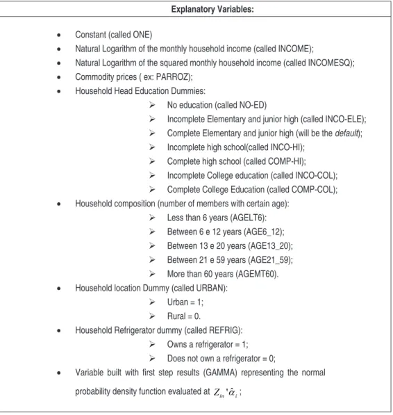
Second step estimation variables are in Table 2.14 Some variables that were used
in the first step are also used in the second, such as monthly household income, education dummies, household location dummy and the refrigerator dummy. The repetition of the first two variables occurs because they are important not only to the purchase decision, but also in the quantity decision. The repetition of the last two variables is justified by the need of a more complete understanding on how these variables impact food demand in Brazil. The second step estimation also in-cludes household composition variables, commonly used in demand studies.15
13 See descriptive statistics for the variables in table a2 in the appendix.
14 all variables except the last are multiplied by the cumulative normal evaluated at the first stage
estimates. See equation (4).
Explanatory Variables:
• Constant (called ONE)
• Natural Logarithm of the monthly household income (called INCOME);
• Natural Logarithm of the squared monthly household income (called INCOMESQ);
• Commodity prices ( ex: PARROZ);
• Household Head Education Dummies:
No education (called NO-ED)
Incomplete Elementary and junior high (called INCO-ELE);
Complete Elementary and junior high (will be the default);
Incomplete high school(called INCO-HI);
Complete high school (called COMP-HI);
Incomplete College education (called INCO-COL);
Complete College Education (called COMP-COL);
• Household composition (number of members with certain age):
Less than 6 years (AGELT6):
Between 6 e 12 years (AGE6_12);
Between 13 e 20 years (AGE13_20);
Between 21 e 59 years (AGE21_59);
More than 60 years (AGEMT60).
• Household location Dummy (called URBAN):
Urban = 1;
Rural = 0.
• Household Refrigerator dummy (called REFRIG):
Owns a refrigerator = 1;
Does not own a refrigerator = 0;
• Variable built with irst step results (GAMMA) representing the normal
probability density function evaluated at Zin'αˆi;
Table 2 – Explanatory Variables Used in the Demand System Estimation Second Step
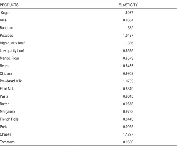
Table 3 – Demand Income Elasticities, Brazil, 2002 - 2003
PRODUCTS ELASTICITY
Sugar 1.8987
Rice 0.8384
Bananas 1.1352
Potatoes 1.0427
High quality beef 1.1336
Low quality beef 0.8375
Manioc Flour 0.8573
Beans 0.8455
Chicken 0.9959
Powdered Milk 1.0763
Fluid Milk 0.8349
Pasta 0.9645
Butter 0.9678
Margarine 0.9752
French Rolls 0.9443
Pork 0.9988
Cheese 1.1297
Tomatoes 0.9586
Source: Estimation results.
The elasticities of staple foods (rice, beans and manioc flour) were bigger than expected, since the initial expectations were that the elasticities were in the [0.1, 0.4] range, even with possibility of negative values. another surprise was the elas-ticities of fluid and powdered milk. Previous studies (hOFFmann, 2000, 2007; mEnEZES et al., 2002) found bigger elasticities for fluid milk and negative elasti-cities for powdered milk, indicating that the latter is an inferior good. Our results show that powdered milk (the most expensive product) is a luxury and fluid milk (the cheapest) is a normal good. This is probably due to the inclusion of the rural territories in Brazil which had been excluded from previous surveys.
(BlUnDEl; PaShaRDES; WEBER, op. cit.). Studies with similar methodology and consumer aggregation to this paper, e.g. Berges e Casellas (2007) for argentina, find expenditure elasticities16 ranging from 0,68 to 2,01, with the majority close to
1 as was the case of this study; b) inclusion of education dummies in both stages. as education was negatively related to the consumption of most food products (even controlling by income effects), especially for staple foods, and as education is gener-ally positive correlated to income, previous studies that did not account for educa-tion should be expected to have smaller income elasticities estimates. addieduca-tional studies using the same methodology are needed to confirm these claims.
Results for marshalian (uncompensated) price elasticities are reported in Table 4. Own-price elasticities are negative for all commodities, with the exception of but-ter. This suggests some problem in estimation perhaps caused by low frequency of consumption of butter in the sample (a little more than 5 %), but such a result is not unusual in large demand systems, e.g. huang (1999).
Other surprising results are the high values of own-price elasticities for staples: rice, beans and manioc flour are price elastic with values as high as -1.98 for manioc flour. meat products, by comparison, have smaller elasticities, ranging from -1.67 (pork) to -0.98 (high quality beef). For other commodities, the majority of de-mands are elastic, with the exceptions of tomatoes (-0.60), margarine (-0.94) and powdered milk (-0.81). although not directly comparable with Berges e Casellas (op. cit.) estimates, since they used more aggregated products, own-price elastici-ties are usually higher here. On the other hand, estimates from alves, menezes and Bezerra (op. cit.) were consistently higher, probably due to the bigger time of adjustment captured by using a pseudopanel.
Results for cross price elasticities show that rice substitutes for pasta, French rolls, potatoes and manioc flour, all alternative carbohydrate sources. Rice is also a com-plement to beans, beef and tomatoes. Beans are substitutes for manioc flour, an unexpected result since their joint consumption is a strong habit in the northeast region. Beans are complements to meat and dairy products (with exception of powdered milk), all alternative sources of protein.
For meats, Table 4 reports that high quality beef is a substitute for chicken and pork. The odd result is the complementary relation between the two types of beef, which are usually regarded as substitutes. Results for milk show the expected substitutability between powdered and fluid milk: a 10% increase in the price of powdered milk causes a 5.58% increase in fluid milk consumption.
16 Income elasticities were also calculated, however as they were calculated by an auxiliary
re B
ra
ga
n
ça c
oe
lh
o, D
an
ilo Ro
lim D
ia
s de a
gu
ia
r, J
am
es s. E
ales
199
E
st. e
co
n., S
ã
o P
au
lo
, 40(1): 185-211, j
an.-m
ar
. 2010
Products Rice Bananas Potatoes High Quality
Beef
Low Quality Beef Manioc Flour Beans Chicken Powdered
Milk
Rice -1.663 0.006 0.300 -0.201 -0.116 0.046 -0.221 0.077 0.047
Bananas 0.050 -1.213 0.094 -0.005 -0.053 -0.143 -0.052 0.243 -0.264
Potatoes 0.156 -0.194 -1.263 -0.119 0.019 0.478 -0.185 -0.238 0.244
High Quality Beef -0.200 0.057 0.224 -0.986 -0.196 -0.272 0.016 0.086 -0.067
Low Quality Beef -0.159 -0.058 0.006 -0.059 -1.279 0.268 0.162 0.168 0.052
Manioc Flour 0.599 0.070 -0.431 -0.422 -0.154 -1.987 0.640 -0.175 0.094
Beans -0.169 0.095 -0.034 0.318 0.186 0.014 -1.255 0.066 -0.068
Chicken 0.030 0.068 0.168 0.010 0.028 -0.155 0.037 -1.132 -0.234
Powdered Milk 0.140 -0.034 0.065 -0.141 0.075 -0.091 -0.052 0.005 -0.810
Fluid Milk 0.108 0.003 -0.047 -0.057 0.078 0.167 0.127 -0.031 0.310
Pasta 0.314 -0.201 -0.324 0.116 0.077 0.034 -0.123 -0.073 -0.241
Butter 0.207 0.093 0.154 -0.463 -0.320 0.058 -0.019 -0.080 0.030
Margarine 0.277 -0.120 -0.033 0.162 0.015 0.185 -0.052 0.015 -0.327
French Rools 0.294 0.105 0.018 0.036 0.158 0.247 0.024 0.007 0.075
Pork 0.055 -0.113 -0.344 0.257 0.181 0.360 0.163 -0.206 0.177
Cheese 0.191 0.097 -0.213 0.030 0.262 -0.116 -0.127 0.310 -0.288
Tomatoes -0.185 0.104 -0.285 -0.075 -0.119 0.371 0.085 0.090 -0.007
co
n., S
ã
o P
au
lo
, 40(1): 185-211, j
an.-m
ar
. 2010
F
o
o
d D
em
a
nd i
n B
ra
zi
l
Products Fluid Milk Pasta Butter Margarine French Rolls Pork Cheese Tomatoes
Rice -0.111 -0.085 -0.660 -0.016 0.270 0.046 -0.297 -0.105
Bananas -0.099 0.040 -0.063 0.115 -0.088 -0.001 0.107 -0.244
Potatoes -0.127 0.008 0.118 0.004 0.125 -0.029 0.012 -0.058
High Quality Beef -0.207 -0.055 -0.393 -0.076 0.101 0.061 0.038 0.075
Low Quality Beef -0.265 0.169 -0.197 0.101 0.050 0.104 0.150 -0.113
Manioc Flour 0.132 -0.039 0.260 -0.332 -0.030 -0.027 0.960 0.621
Beans 0.068 -0.363 0.190 -0.075 0.015 0.060 -0.150 -0.171
Chicken -0.006 0.024 -0.102 0.025 -0.171 -0.134 0.120 -0.039
Powdered Milk 0.558 0.125 0.099 -0.243 -0.192 -0.013 0.147 0.030
Fluid Milk -1.129 0.169 0.002 0.206 0.067 0.142 -0.052 0.007
Pasta 0.238 -1.384 0.089 -0.410 -0.100 -0.104 -0.006 -0.259
Butter 0.542 -0.103 0.402 0.656 0.289 -0.163 -0.021 -0.207
Margarine 0.351 -0.245 0.091 -0.947 -0.149 -0.047 -0.033 -0.156
French Rools 0.154 0.082 0.410 0.051 -1.175 0.122 0.022 0.018
Pork -0.188 0.133 0.137 0.010 0.199 -1.677 -0.001 0.214
Cheese 0.095 0.045 0.243 -0.067 0.036 0.294 -1.283 0.005
5 Conclusions
Several interesting features of Brazilian demand for food products have been pre-sented. In general, the larger is a family’s income, the smaller is the probability of purchasing staple foods and the larger is the probability of purchasing meat, milk and other products as would be expected.
Regional variables were also important in the demand system. They were important not only for the so called “regional foods”, such as manioc flour in the north and northeast or beef in the South, but also for almost all the commodities.
Women’s role as household heads is also important in understanding differences in food consumption. Results show that there is a smaller purchase probability for almost all goods in our sample when women are household heads. The reason is straightforward: when women work, meals away from home are substituted for at home meals.
Second stage results were more problematic than the first stage ones. Estimated income elasticities showed all goods were normal. Sugar, high quality beef, bananas, cheese and powdered milk were found to be luxuries. Some staples were more pri-ce elastic than expected. Cross pripri-ce elasticities results agreed with expectations, for the most part.
This paper main contribution was to account for the zero expenditure problem usually overlooked in similar studies but always present when we deal with a large household consumption data. Results showed that elasticities were generally higher when we consider this issue. a limitation of our analysis is the low number of fruits and vegetables in the sample, not allowing a more careful analysis about the role of health concerns in food consumption patterns. another issue which we do not deal with is the infrequency of purchase problem, i.e., the observed zero consumption by a household may be a result of infrequency of purchases and not a corner solu-tion. Further research is needed to incorporate these issues in the Brazilian food demand system estimation.
References
aGUERO, J. m.; GOUlD, B. W. household composition and Brazilian food
pur-chases: an expenditure system approach. Canadian Journal of Agriculture
Economics, v. 51, n. 3, p. 323-345, 2003.
alVES, D., mEnEZES T.; BEZERRa, F. Estimação do sistema de demanda censurada
l. m. S.; mEnEZES, T.; PIOla, S. F. (Org.). Gasto e consumo das famílias
brasileiras contemporâneas. Brasília: IPEa, p. 395-422, 2007. v. 2.
BaCChI, m.R.P. Demanda de carne bovina no mercado brasileiro. 1989. Piracicaba,
ESalQ/USP, 77p. (unpublished master dissertation).
BanKS, J.; BlUnDEll, R.; lEWBEl, a. Quadratic Engel curves and consumer
demand. The Review of Economics and Statistics, v. lXXIX, n. 4, p.527-539,
nov. 1997.
BaTalha, m.O.; lUCChESE, T.; lamBERT, J.l. hábitos de consumo alimentar
no Brasil: realidade e perspectivas. In: BaTalha, mario O. (Coord.). Gestão
do Agronegócio – Textos selecionados. São Carlos: Edufscar, 2005.
BERGES, m; CaSEllaS, K. Estimación de um sistema de demanda de alimentos: um análisis aplicado a hogares pobres y no pobres. In: SIlVEIRa, F. G.; SERVO,
l. m. S.; mEnEZES, T.; PIOla, S. F. (Org.). Gasto e consumo das famílias
brasileiras contemporâneas. Brasília: IPEa, p.529-551, 2007. v. 2.
BlUnDEll, R.; PaShaRDES, P.; WEBER, G. What do we learn about consumer
demand patterns from microdata. American Economic Review, 83 (3),
p.570-597, June 1993.
DOnG, D.; GOUlD, B.W.; KaISER, h.m. Food demand in mexico: an application of the amemiya-Tobin approach to the estimation of a censored food system.
American Journal of Agriculture Economics, v. 86, n. 4, p. 1094-1107, 2004.
FURTUOSO, m. C. O. Redistribuição de e consumo de Alimentos no Estado de São
Paulo. 1981. Piracicaba, ESalQ/USP, 106p. (unpublished master
disserta-tion).
GREEnE, W.h. Econometric analysis.Prentice hall, Upper Saddle River, Fourth
edition, 2000, 1004p.
haInES, P. S.; GUIlKEY, D. K.; POPKIn, B.m. modeling food consumption
deci-sions as a two-step process.American Journal of Agricultural Economics, v. 70,
n. 3, p. 543-552, aug. 1988.
hEIEn, D.; WESSElS, C.R. Demand systems estimation with microdata: a
cen-sored regression approach. Journal of Business and Economic Statistics, v. 8, n.
3, July 1990.
hOFFmann, R. a diminuição do consumo de feijão no Brasil. Estudos Econômicos,
v. 25, n. 2, p. 189-201, maio-ago. 1995.
______. Elasticidades-renda das despesas e do consumo físico de alimentos no Brasil
metropolitano em 1995-96. Agricultura em São Paulo, SP, v. 47, n. 1 p.
111-122, 2000.
______. Elasticidades-renda das despesas e do consumo de alimentos no Brasil em 2002-2003. In: SIlVEIRa, F. G.; SERVO, l. m. S.; mEnEZES, T.; PIOla, S.
F. (Org.). Gasto e consumo das famílias brasileiras contemporâneas. Brasília:
hUanG, K. Effects of food prices and consumer income on nutrient availability.
Applied Economics, 31, p. 367-380, 1999.
IBGE. Pesquisa de Orçamentos Familiares 2002-2003. aquisição alimentar
domi-ciliar per capita: Brasil e grandes regiões. Rio de Janeiro: Instituto Brasileiro de Geografia e Estatística, 2004a.
______. Pesquisa de Orçamentos Familiares 2002-2003. CD-ROm -microdados
– Segunda divulgação. Rio de Janeiro: Instituto Brasileiro de Geografia e Esta-tística, 2004b.
lEE, l. F; PITT, m. m. microeconometric demand systems with binding
nonnega-tivity constraints: the dual approach. Econometrica, v. 54, n. 5, p. 1237-1242,
Sep. 1986.
manChESTER, a. C. household consumption behavior: understanding,
mea-surement, and applications in policy-oriented research. American Journal of
Agricultural Economics, v. 59, n. 1, p. 149-154, Feb. 1977.
mEnEZES, T.; SIlVEIRa, F. G; aZZOnI, C.R. Demand elasticities for food
products: a two-stage budgeting system. nEREUS-USP, São Paulo, 2005 (TD
nereus 09-2005).
mEnEZES, T.; SIlVEIRa, F. G; maGalhÃES, l.C.G.; TOmICh, F.a.;VIanna,
S.W. Gastos alimentares nas grandes regiões urbanas do Brasil: aplicação do
modelo aID aos microdados da POF 1995/1996 IBGE. Brasília: IPEa, 2002 (Discussion Paper, n. 896).
mURPhY, K. m.; TOPEl, R. h. Estimation and inference in two-step
econome-tric models. Journal of Business and Economic Statistics 3, p. 370-379, Oct.
1985.
ShOnKWIlER, J. S.; YEn, S.T. Two-step estimation of a censored system of equa-tions. American Journal of Agricultural Economics. v. 81, n. 4, p. 972-982, nov. 1999.
SIlVEIRa, F. G.; mEnEZES, T.; maGalhÃES, l.C.G.; DInIZ, B. P. C. Elasti-cidade-renda dos produtos alimentares nas regiões metropolitanas brasileiras:
uma aplicação da POF 1995/1996. Estudos Econômicos, v. 37, n. 2, p. 329-352,
2007a.
SIlVEIRa, F. G.; SERVO, l. m. S.; mEnEZES, T.; PIOla, S. F. Gasto e consumo
das famílias brasileiras contemporâneas. Brasília: IPEa, 2007b, 551 p. v. 2.
ThOmaS, D.; STRaUSS, J.; BaRBOSa, m. m. T. Estimativas do impacto de
mudanças de renda e de preços no consumo no Brasil. Pesquisa e Planejamento
Econômico, v. 21, n. 2, p. 305-354, 1991.
WalES, T. J.; WOODlanD, a. D. Sample selectivity and the estimation of labor
supply functions. International Economic Review, v. 21, n. 2, p. 437-468, June
YEn, S. T; hUanG, C. l. Cross-sectional estimation of U. S. demand for beef
products: a censored system approach. Journal of Agricultural and Resource
Economics, v. 27, n. 2, p. 320-334, 2002.
YEn, S.T.; Kan, K.; SU, S. household demand of fats and oil: two-step estimation
of a censored demand system. Applied Economics, v. 34, n. 14, p. 1799-1806,
re B
ra
ga
n
ça c
oe
lh
o, D
an
ilo Ro
lim D
ia
s de a
gu
ia
r, J
am
es s. E
ales
205
E
st. e
co
n., S
ã
o P
au
lo
, 40(1): 185-211, j
an.-m
ar
. 2010
Table A1 – First Step Estimation Results (purchase decision results), Brazil, 2002 - 2003
Sugar Rice Bananas Potatoes High Quality Beef Low Quality Beef
Variable Coef. Std. Err. Coef. Std. Err. Coef. Std. Err. Coef. Std. Err. Coef. Std. Err. Coef. Std. Err.
One -0.042 0.063 0.037 0.063 -2.087** 0.067 -2.051** 0.070 -2.704** 0.072 -1.106** 0.066
Income -0.047** 0.008 -0.051** 0.008 0.182** 0.009 0.179** 0.009 0.235** 0.009 0.024** 0.009
North 0.351** 0.023 0.497** 0.023 0.009 0.024 -0.317** 0.026 0.396** 0.025 0.402 0.024
Northeast 0.550** 0.019 0.530** 0.019 0.286** 0.020 -0.082** 0.020 0.129** 0.021 0.128** 0.020
South -0.002 0.024 0.071** 0.024 0.053** 0.024 0.083** 0.024 0.000 0.026 0.230** 0.024
Center-W -0.045** 0.022 0.103** 0.022 -0.208** 0.023 -0.286** 0.024 0.118** 0.024 0.168** 0.023
Urban -0.146** 0.016 -0.091** 0.016 0.139** 0.018 0.059** 0.019 0.108** 0.019 0.107** 0.017
No-Ed 0.155** 0.028 0.094** 0.027 -0.059** 0.029 -0.181** 0.031 -0.124** 0.031 0.043 0.029
Inco-Ele 0.122** 0.024 0.102** 0.023 -0.044* 0.025 -0.065** 0.025 -0.045* 0.026 0.010 0.024
Inco-Hi -0.029 0.037 -0.042 0.037 -0.029 0.038 -0.035 0.039 0.051 0.039 -0.005 0.038
Comp-Hi -0.079** 0.028 -0.101** 0.028 -0.005 0.029 -0.022 0.030 0.040 0.030 -0.138** 0.029
Inco-Col -0.251** 0.049 -0.292** 0.048 -0.042 0.047 -0.104** 0.049 -0.070* 0.048 -0.317** 0.051
Comp-Col -0.086** 0.039 -0.188** 0.039 -0.022 0.038 -0.153** 0.040 -0.101** 0.039 -0.335** 0.042
Black 0.035 0.026 0.050* 0.026 -0.155** 0.029 -0.137** 0.030 -0.200** 0.031 0.100** 0.027
Asian -0.085 0.101 0.059 0.097 -0.088 0.102 -0.035 0.104 0.189* 0.098 0.126 0.100
Mixed 0.058** 0.014 0.065** 0.014 -0.054** 0.015 -0.048** 0.016 -0.075** 0.016 0.056** 0.015
Other -0.126 0.085 -0.223** 0.084 -0.092 0.090 -0.107 0.098 -0.052 0.093 -0.099 0.090
Woman -0.088** 0.015 -0.148** 0.014 0.029* 0.015 -0.011 0.016 -0.034** 0.016 -0.070** 0.015
Domestic -0.043* 0.024 -0.008 0.024 0.084 0.024 0.078** 0.025 0.129** 0.024 -0.093** 0.025
Refrig -0.112** 0.018 -0.130** 0.018 0.127 0.020 0.239** 0.022 0.210** 0.022 0.109** 0.019
Obs: Coefficients in bold type are significant at 5 % (**) & 10 % (*).
co
n., S
ã
o P
au
lo
, 40(1): 185-211, j
an.-m
ar
. 2010
F
o
o
d D
em
a
nd i
n B
ra
zi
l
Manioc Flour Beans Chicken Powdered Milk Fluid Milk Pasta
Variáble Coef. Std. Dev. Coef. Std. Dev. Coef. Std. Dev. Coef. Std. Dev. Coef. Std. Dev. Coef. Std. Dev.
One -1.092** 0.074 -0.365** 0.063 -1.228** 0.063 -1.953** 0.078 -0.832** 0.063 -0.893** 0.065
Income -0.014 0.010 -0.003 0.008 0.117** 0.008 0.036** 0.010 0.143** 0.008 0.032** 0.008
North 1.054** 0.027 0.271** 0.023 0.227** 0.022 1.072** 0.029 -0.549** 0.023 0.071** 0.024
Northeast 0.829** 0.024 0.526** 0.019 0.255** 0.019 0.978** 0.026 -0.461** 0.019 0.250** 0.019
South -0.255** 0.036 0.055** 0.024 0.069** 0.023 -0.117** 0.038 0.135** 0.023 0.104** 0.024
Center-W -0.211** 0.031 0.032 0.022 -0.121** 0.022 -0.160** 0.035 0.125** 0.021 -0.079** 0.023
Urban -0.135** 0.018 -0.200** 0.016 -0.024 0.016 0.248** 0.021 -0.130** 0.016 0.009 0.017
No-Ed 0.210** 0.033 0.169** 0.028 -0.004 0.027 -0.185** 0.034 -0.071** 0.028 -0.044 0.028
Inco-Ele 0.141** 0.029 0.123** 0.024 0.054** 0.023 -0.075** 0.029 0.013 0.024 0.039 0.024
Inco-Hi 0.027 0.045 -0.062* 0.038 -0.071* 0.036 -0.001 0.044 -0.009 0.037 0.024 0.038
Comp-Hi -0.051 0.035 -0.120** 0.029 -0.115** 0.028 0.025 0.034 -0.036 0.028 -0.013 0.029
Inco-Col -0.223** 0.063 -0.303** 0.050 -0.307** 0.047 -0.181** 0.060 -0.145** 0.046 -0.162** 0.049
Comp-Col -0.189** 0.052 -0.177** 0.040 -0.296** 0.038 -0.001 0.047 -0.158** 0.038 -0.084** 0.039
Black 0.171** 0.030 0.011 0.027 0.056** 0.026 0.119** 0.032 -0.202** 0.027 -0.072** 0.028
Asian 0.018 0.126 -0.140 0.103 -0.047 0.097 -0.040 0.133 -0.305** 0.096 -0.099 0.102
Mixed 0.094** 0.016 0.045** 0.014 0.031** 0.014 0.080** 0.017 -0.147** 0.014 0.003 0.015
Other 0.004 0.095 -0.239** 0.087 -0.188** 0.085 -0.076 0.103 -0.311** 0.087 -0.138 0.089
Woman -0.096** 0.017 -0.149** 0.015 -0.040** 0.014 0.007 0.017 -0.007 0.014 -0.075** 0.015
Domestic -0.160** 0.030 -0.043* 0.024 -0.052** 0.023 0.001 0.029 0.050** 0.024 -0.018 0.024
Refrig -0.170** 0.019 -0.086** 0.018 0.113** 0.018 -0.068** 0.021 0.269** 0.018 0.054** 0.019
Obs: Coefficients in bold type are significant at 5 % (**) & 10 % (*).
re B
ra
ga
n
ça c
oe
lh
o, D
an
ilo Ro
lim D
ia
s de a
gu
ia
r, J
am
es s. E
ales
207
E
st. e
co
n., S
ã
o P
au
lo
, 40(1): 185-211, j
an.-m
ar
. 2010
Butter Margarine French Rolls Pork Cheese Tomatoes
Variable Coef. Std. Dev. Coef. Std. Dev. Coef. Std. Dev. Coef. Std. Dev. Coef. Std. Dev. Coef. Std. Dev.
One -2.800** 0.104 -2.040** 0.071 -1.537** 0.066 -1.134** 0.066 -3.498** 0.083 -1.987** 0.066
Income 0.148** 0.013 0.119** 0.009 0.197** 0.009 0.117** 0.009 0.352** 0.010 0.157** 0.008
North 0.109** 0.033 0.198** 0.026 -0.177** 0.024 -0.412** 0.024 -0.390** 0.030 0.097** 0.024
Northeast 0.018 0.028 0.447** 0.021 0.031 0.020 -0.253** 0.019 -0.103** 0.022 0.410** 0.019
South -0.546** 0.044 0.176** 0.026 -0.523** 0.024 0.119** 0.023 0.013 0.026 -0.068** 0.024
Center-W -0.480** 0.039 -0.015 0.025 -0.403** 0.022 -0.401** 0.022 -0.284** 0.026 -0.028 0.023
Urban 0.157** 0.029 0.122** 0.019 0.744** 0.016 -0.011 0.017 0.082** 0.023 0.146** 0.017
No-Ed -0.127** 0.047 -0.198** 0.031 -0.357** 0.029 -0.088** 0.029 -0.350** 0.037 -0.111** 0.029
Inco-Ele -0.009 0.039 -0.033 0.026 -0.164** 0.025 0.009 0.024 -0.177** 0.028 -0.025 0.024
Inco-Hi 0.085 0.057 0.019 0.040 -0.022 0.039 -0.009 0.038 0.034 0.043 0.028 0.037
Comp-Hi 0.059 0.044 -0.002 0.030 0.082** 0.030 -0.048** 0.029 0.114** 0.032 -0.029 0.028
Inco-Col 0.055 0.069 -0.123** 0.050 -0.123** 0.050 -0.154** 0.048 0.158** 0.049 -0.067 0.047
Comp-Col 0.052 0.056 -0.090** 0.041 -0.117** 0.042 -0.161** 0.039 0.219** 0.040 -0.121** 0.038
Black 0.073* 0.043 -0.036 0.030 -0.054** 0.027 0.047* 0.027 -0.166** 0.035 -0.065** 0.028
Asian -0.139 0.170 -0.303** 0.119 0.024 0.101 0.109 0.099 -0.236** 0.115 0.208** 0.096
Mixed 0.032 0.023 -0.014 0.016 -0.010 0.015 0.026* 0.015 -0.180** 0.018 -0.008 0.015
Other 0.003 0.140 -0.245** 0.103 -0.215** 0.089 -0.173** 0.094 -0.324** 0.124 -0.180** 0.092
Woman 0.024 0.023 0.000 0.016 0.042** 0.015 -0.071** 0.015 0.058** 0.018 -0.051** 0.015
Domestic 0.082** 0.034 -0.082** 0.026 -0.063** 0.026 -0.041** 0.025 0.074** 0.026 0.059** 0.024
Refrig 0.116** 0.032 0.190** 0.021 0.355** 0.018 -0.015 0.019 0.285** 0.029 0.205** 0.019
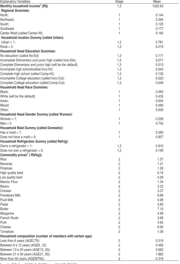
Table A2 – Descriptive Statistics of Variables
Explanatory Variables: Stage Mean
Monthly household income1 (R$)
1,2 1525.63 Regional Dummies:
North; 1 0.144
Northeast; 1 0.394
South; 1 0.125
Southeast 1 0.177
Center-West (called Center-W); 1 0.160 Household location Dummy (called Urban):
Urban = 1; 1,2 0.781
Rural = 0. 1,2 0.219
Household Head Education Dummies:
No education (called No-Ed) 1,2 0.171
Incomplete Elementary and junior high (called Inco-Ele); 1,2 0.071 Complete Elementary and junior high (will be the default); 1,2 0.513
Incomplete high school(called Inco-Hi); 1,2 0.043 Complete high school (called Comp-Hi); 1,2 0.130 Incomplete College education (called Inco-Col); 1,2 0.023 Complete College education (called Comp-Col); 1,2 0.049 Household Head Race Dummies:
Black; 1 0.065
White (will be the default); 1 0.435
Asian; 1 0.004
Mixed; 1 0.490
Other; 1 0.005
Household Head Gender Dummy (called Woman):
Woman = 1; 1 0.258
Man = 0 1 0.742
Household Maid Dummy (called Domestic):
Has a maid = 1; 1 0.093
Does not have a maid = 0; 1 0.907
Household Refrigerator dummy (called Refrig):
Owns a refrigerator = 1; 1,2 0.810
Does not own a refrigerator = 0; 1,2 0.190 Commodity prices1 ( R$/kg));
Rice 2 1.57
Bananas 2 1.21
Potatoes 2 1.28
High quality beef 2 6.19
Low quality beef 2 4.26
Manioc Flour 2 1.34
Beans 2 2.23
Chicken 2 3.37
Powdered Milk 2 9.88
Fluid Milk 2 0.99
Pasta 2 3.85
Butter 2 7.10
Margarine 2 4.99
French Rools 2 3.68
Pork 2 4.64
Cheese 2 8.92
Tomatoes 2 1.09
Household composition (number of members with certain age):
Less than 6 years (AGELT6): 2 0.519
Between 6 e 12 years (AGE6_12); 2 0.482 Between 13 e 20 years (AGE13_20); 2 0.662 Between 21 e 59 years (AGE21_59); 2 1.862
More than 60 years (AGEMT60). 2 0.318
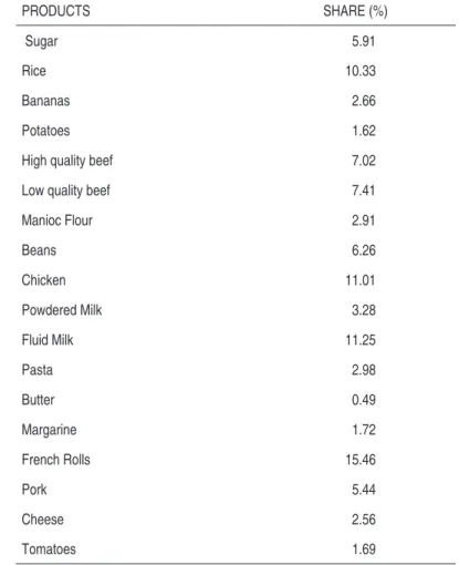
Table A3 – Total Expenditure Average Share of the Eighteen Food Products, Brazil, 2002-2003
PRODUCTS SHARE (%)
Sugar 5.91
Rice 10.33
Bananas 2.66
Potatoes 1.62
High quality beef 7.02
Low quality beef 7.41
Manioc Flour 2.91
Beans 6.26
Chicken 11.01
Powdered Milk 3.28
Fluid Milk 11.25
Pasta 2.98
Butter 0.49
Margarine 1.72
French Rolls 15.46
Pork 5.44
Cheese 2.56
Tomatoes 1.69
co
n., S
ã
o P
au
lo
, 40(1): 185-211, j
an.-m
ar
. 2010
F
o
o
d D
em
a
nd i
n B
ra
zi
l
States
Average state prices (R$/kg)
Sugar Rice Bananas Potatoes High quality
beef Low quality beef Manioc lour Beans Chicken
Acre 1.42 1.60 0.97 1.82 4.98 3.42 1.08 2.34 3.66
Alagoas 1.11 1.66 1.40 1.19 6.02 4.14 1.25 2.04 3.46
Amapá 1.39 1.62 1.69 1.57 5.69 3.97 1.09 2.75 3.07
Amazonas 1.37 1.71 1.38 1.95 5.69 3.93 1.21 2.55 3.08
Bahia 1.29 1.70 1.18 1.20 6.45 4.68 1.22 2.14 3.57
Ceará 1.27 1.62 1.08 1.44 6.29 4.51 0.97 1.89 3.44
Distrito Federal 1.26 1.47 1.39 1.43 7.12 4.35 1.61 2.32 3.41
Espírito Santo 1.14 1.56 0.92 1.17 6.67 4.36 1.39 2.24 3.10
Goiás 1.22 1.50 1.51 1.39 6.29 4.57 1.73 2.45 3.14
Maranhão 1.38 1.32 1.21 1.43 4.93 3.50 1.10 2.22 3.69
Mato Grosso 1.34 1.34 2.29 1.50 5.76 4.07 1.94 2.33 3.33
Mato Grosso do Sul 1.29 1.46 1.22 1.29 5.94 4.13 1.59 2.32 2.97
Minas Gerais 1.16 1.55 1.10 1.04 6.83 4.67 1.19 2.31 3.28
Pará 1.41 1.55 1.05 1.51 5.39 3.70 0.97 2.49 3.39
Paraíba 1.18 1.71 1.07 1.16 6.75 4.74 1.32 2.07 3.65
Paraná 1.18 1.55 0.82 0.97 6.29 4.20 1.55 2.17 1.13
Pernambuco 1.15 1.74 1.43 1.31 5.98 4.37 1.30 2.22 3.66
Piauí 1.31 1.34 1.28 1.35 6.03 4,00 1,00 1.99 3.55
Rio de Janeiro 1.35 1.69 1.29 1.11 7.07 4.82 1.46 2.21 3.69
Rio Grande do Norte 1.26 1.71 1.03 1.23 6.77 4.46 1.12 2.19 3.64
Rio Grande do Sul 1.50 1.57 1,00 1.03 6.27 4.18 1.51 2.14 3.10
Rondônia 1.27 1.52 1.18 1.36 5.26 3.64 1.32 2.13 3.06
Roraima 1.31 1.38 1.29 2.27 6.58 4.20 1.50 2.60 3.48
Santa Catarina 1.44 1.59 0.85 0.93 6.03 4.08 1.44 2.07 3.04
São Paulo 1.24 1.61 1.07 1.14 7.15 4.66 1.63 2.48 3.46
Sergipe 1.21 1.78 1.03 1.14 6.52 4.44 1.49 2.14 3.73
Tocantins 1.44 1.54 1.22 1.49 5.71 4,00 1.28 2.59 3.48
re B
ra
ga
n
ça c
oe
lh
o, D
an
ilo Ro
lim D
ia
s de a
gu
ia
r, J
am
es s. E
ales
211
E
st. e
co
n., S
ã
o P
au
lo
, 40(1): 185-211, j
an.-m
ar
. 2010
States
Average state prices (R$/kg) Powdered
Milk Fluid Milk Pasta Butter Margarine French Rolls Pork Cheese Tomatoes
Acre 9.75 1.02 4.74 8.84 6.64 3.88 5.43 8.48 1.79
Alagoas 8.69 1.06 3.30 7.22 4.57 3.04 3.66 9.51 0.86
Amapá 9.30 1.76 3.92 5.80 5.18 3.67 5.07 9.45 1.67
Amazonas 9.80 1.30 3.36 7.61 5.33 3.34 5.48 9.12 2.04
Bahia 9.75 0.91 3.04 9.20 4.55 3.16 4.96 11.29 0.96
Ceará 9.73 1.07 3.31 6.80 4.75 3.28 4.30 8.22 1.02
Distrito Federal 10.99 1.11 5.19 9.28 5.28 4.35 5.64 11.18 1.10
Espírito Santo 11.20 0.98 3.93 8.26 5.48 4.29 4.93 9.15 0.87
Goiás 11.02 0.83 3.80 5.78 4.65 4.49 5.16 6.47 1.12
Maranhão 9.28 0.85 4.38 4.94 4.87 3.21 3.70 8.90 1.07
Mato Grosso 10.20 0.89 3.91 6.55 5.54 4.37 4.61 8.03 1.22
Mato Grosso do Sul 9.94 0.87 4,00 5.88 4.91 3.86 4.65 8.23 1.08
Minas Gerais 11.07 0.86 3.61 7.77 5.15 3.97 4.77 7.18 0.95
Pará 9.26 0.85 3.88 6.80 4.82 3.77 4.50 9.59 1.55
Paraíba 9.30 0.99 2.98 7.28 4.57 3.03 4.22 8.41 0.84
Paraná 10.24 0.96 3.84 8.77 4.64 3.63 4.66 10.11 0.97
Pernambuco 8.78 1.06 3.02 8.26 4.41 2.91 4.09 8.33 0.87
Piauí 8.83 1.12 4.16 5.78 4.81 3.61 4.15 8.81 1,00
Rio de Janeiro 9.95 1.29 4.53 9.32 5.58 4.07 5.50 9.99 1.05
Rio Grande do Norte 9.71 1.06 3.07 7.88 5.09 3.10 3.72 9.09 0.88
Rio Grande do Sul 9.92 1.02 4.36 6.54 4.96 3.86 5.28 10.40 1.24
Rondônia 10.04 0.82 4.21 6.62 5.54 3.75 4.29 7.51 1.21
Roraima 9.64 1.34 4.93 6.15 5.51 3.94 5.50 10.86 1.77
Santa Catarina 10.31 0.99 4.54 5.37 5.07 4.04 4.69 8.39 1.06
São Paulo 9.55 1.15 4.58 6.97 5.01 3.95 5.82 10.67 1.18
Sergipe 10.36 0.97 4.14 7.08 5.05 2.96 4.27 9.39 0.92