UMA EXTENSÃO SQL PARA O SUPORTE DE
LUÍS EDUARDO OLIVEIRA LIZARDO
UMA EXTENSÃO SQL PARA O SUPORTE DE
TIPOS DE DADOS ESPACIAIS AVANÇADOS E
RESTRIÇÕES DE INTEGRIDADE
Dissertação apresentada ao Programa de Pós-Graduação em Ciência da Computação do Instituto de Ciências Exatas da Univer-sidade Federal de Minas Gerais como req-uisito parcial para a obtenção do grau de Mestre em Ciência da Computação.
Orientador: Clodoveu Augusto Davis Junior
LUÍS EDUARDO OLIVEIRA LIZARDO
A SQL EXTENSION TO SUPPORT ADVANCED
SPATIAL DATA TYPES AND INTEGRITY
CONSTRAINTS
Dissertation presented to the Graduate Program in Computer Science of the Uni-versidade Federal de Minas Gerais in par-tial fulfillment of the requirements for the degree of Master in Computer Science.
Advisor: Clodoveu Augusto Davis Junior
© 2017, Luís Eduardo Oliveira Lizardo. Todos os direitos reservados.
Lizardo, Luís Eduardo Oliveira
L789s A SQL extension to support advanced spatial data types and integrity constraints / Luís Eduardo Oliveira Lizardo. — Belo Horizonte, 2017
xxviii, 63 f. : il. ; 29cm
Dissertação (mestrado) — Universidade Federal de Minas Gerais
Orientador: Clodoveu Augusto Davis Junior
1. Computação – Teses. 2. Sistemas de informação geográfica. 3. Banco de dados espaciais. 4. Modelagem de banco de dados. I. Orientador. II. Titulo.
In memory of my grandfathers:
Acknowledgments
I would like to thank my advisor and professor Clodoveu. Without his excellent guid-ance, patience and constant support, this work wouldn’t have been completed.
For all the classes and technical learning, I am especially thankful for the pro-fessors and teachers, from EMNSA, CEFET-MG, FH-S and UFMG. Without your knowledge and patience I would not be finishing this important step in my life.
I would like to express my deep gratitude to my mother Alzira, who has inspired and motivated me all the times to achieve my goals. I owe you everything that I am today. I am extremely fortunate to be so blessed.
To my dear friends, I am very grateful to each of the tiny moments that we’ve spent together. The help and understanding of each one of you have been essential to my growth. Every moment with you is an eternal bond, and this is noticed in the human being each of us are and have become.
Resumo
As primitivas geométricas definidas pelos padrões OGC e ISO, implementadas na maio-ria dos sistemas gerenciadores de banco de dados (SGBD) com suporte para dados es-paciais, são incapazes de capturar a semântica de tipos ricos de representação, como os encontrados nos atuais modelos de dados geográficos. Além disso, os SGBDs relacionais não estendem os mecanismos de integridade referencial para cobrir relações espaciais e para suportar restrições de integridade espacial. Em vez disso, eles geralmente assumem que toda a verificação de integridade espacial será realizada pela aplicação, durante o processo de entrada de dados. Além de não ser prático, se o DBMS suportar muitas aplicações, isto pode levar a implementações redundantes e inconsistentes. Por isso, este trabalho apresenta o AST-PostGIS, uma extensão para PostgreSQL/PostGIS que incorpora à Linguagem SQL tipos de dados espaciais avançados e implementa restrições de integridade espaciais. A extensão reduz a distância entre os projetos conceituais e físicos de banco de dados espaciais, fornecendo representações ricas para geometrias do tipo geo-objeto e geo-campo. Ele também oferece funções para garantir a consistência das relações espaciais durante as atualizações de dados. Outras funções podem ainda ser utilizadas antes de impor restrições de integridade espacial pela primeira vez para verificar a consistência inicial do banco de dados. O uso do AST-PostGIS é ilustrado em um pequeno projeto de banco de dados geográfico urbano, mapeando seu esquema conceitual para a implementação física em SQL estendido.
Abstract
Geometric primitives defined by OGC and ISO standards, implemented in most modern spatially-enabled database management systems (DBMS), are unable to capture the semantics of richer representation types, as found in current geographic data models. Moreover, relational DBMSs do not extend referential integrity mechanisms to cover spatial relationships and to support spatial integrity constraints. Rather, they usually assume that all spatial integrity checking will be carried out by the application, during the data entry process. This is not practical if the DBMS supports many applications, and can lead to redundant and inconsistent work. Therefore, this work presents AST-PostGIS, an extension for PostgreSQL/PostGIS that incorporates advanced spatial data types and implements spatial integrity constraints. The extension reduces the distance between the conceptual and the physical designs of spatial databases, by providing richer representations for geo-object and geo-field geometries. It also offers procedures to assert the consistency of spatial relationships during data updates. Such procedures can also be used before enforcing spatial integrity constraints for the first time. We illustrate the use of AST-PostGIS on an urban geographic database design problem, by mapping its conceptual schema to the physical implementation in extended SQL.
List of Figures
2.1 DE-9IM over spatial object interactions. . . 8
2.2 Conceptual diagram for a spatial RDBMS. . . 10
3.1 Simplified graphical notation of a class in OMT-G. . . 18
3.2 Geo-object classes . . . 19
3.3 Geo-field classes . . . 19
3.4 OMT-G notations for relationships. . . 21
3.5 OMT-G notations for generalizations and aggregations. . . 22
4.1 AST-PostGIS log table schema . . . 35
5.1 OMT-G schema fragment for an urban geographic application . . . 38
5.2 Overview of urban scenario without integrity constraints violations. . . 44
5.3 Spatial aggregation violation: a parcel extrapolates the block limits. . . 44
5.4 AST-PostGIS response for a spatial aggregation violation. . . 45
5.5 Spatial relationship violation: building is not within the parcel area. . . 45
5.6 AST-PostGIS response for a spatial relationship integrity constraint violation. 46 5.7 Arc-Node network violation: streets segments (arcs) do not intersect cross-ings (nodes) . . . 46
List of Tables
3.1 Geometric types: OMT-G and OGC SFS . . . 27
4.1 Advanced spatial data types supported by AST-PostGIS . . . 30 4.2 Consistency check functions supported by AST-PostGIS . . . 34
List of Listings
4.1 Aggregation Trigger . . . 32 4.2 Arc-Node Trigger . . . 32 4.3 Spatial Relationship Trigger . . . 33 4.4 Usage of the consistency check function for network relationship . . . 34
5.1 SQL schema for the tables definition . . . 41 5.2 Integrity constraints implementation for aggregations . . . 41 5.3 Integrity constraints implementation for spatial relationships . . . 42 5.4 Integrity constraint implementation for arc-node network . . . 43
Acronyms
ACID: Atomicity, Consistency, Isolation, Durability
AST: Advanced Spatial Type
DBMS: Database Management System
DDL: Data Definition Language
DE-9IM: Dimensionally-Extended Nine-Intersection Model
ER: Entity–Relationship
GIS: Geographic information system
GML: Geography Markup Language
ISO: International Organization for Standardization
MVCC: Multi-Version Concurrency Control
OGC: Open Geospatial Consortium
OMT-G: Object Modeling Technique for Geographic Applications
OMT: Object Modeling Technique
PL/pgSQL: Procedural Language/PostgreSQL
RDBMS: Relational Database Management System
SFS4SQL: Simple Features Specification for SQL
SRID: Spatial Reference System Identifier
TCL: Tool Command Language
TIN: Triangular Irregular Network
UML: Unified Modeling Language
XML: Extensible Markup Language
Contents
Acknowledgments xi
Resumo xv
Abstract xvii
List of Figures xix
List of Tables xxi
List of Listings xxiii
Acronyms xxv
1 Introduction 1
1.1 Contributions and objective . . . 3 1.2 Work outline . . . 4
2 Related Work 5
2.1 Spatial data . . . 5 2.2 Spatial relationships . . . 7 2.3 Spatial integrity constraints . . . 8 2.4 Spatial database management systems . . . 9 2.4.1 PostgreSQL Overview . . . 11 2.5 Conceptual modeling for spatial databases . . . 13
3 The OMT-G Model 17
3.2 Integrity Constraints . . . 21 3.2.1 Geo-field constraints . . . 22 3.2.2 Geo-object constraints . . . 23 3.2.3 Network relationship constraints . . . 24 3.2.4 Spatial aggregation constraint . . . 24 3.2.5 Spatial relationship constraints . . . 25 3.3 Mapping OMT-G to object-relational spatial databases . . . 27 3.4 Further work on OMT-G . . . 28
4 AST-PostGIS 29
4.1 Advanced Spatial Data Types . . . 30 4.2 Integrity constraints for spatial relationships . . . 30 4.3 Consistency Check Functions . . . 34 4.4 Summary of limitations . . . 35
5 Case Study: Urban geographic database 37
5.1 Conceptual schema . . . 37 5.2 Physical implementation . . . 39 5.3 AST-PostGIS responses . . . 43 5.3.1 Spatial aggregation violation . . . 44 5.3.2 Spatial relationship violation . . . 45 5.3.3 Arc-node network violation . . . 45
6 Conclusions and Future Work 47
Bibliography 49
Appendix A SQL schema for the urban cadastral database 57
Chapter 1
Introduction
OpenGIS (OGC) and SQL/MM (ISO) standards have been instrumental in the effort to standardize spatial data management using relational and object-relational databases. OpenGIS, the set of spatial data standards proposed by the Open Geospa-tial Consortium (OGC), covers many aspects of spaGeospa-tial data representation, spaGeospa-tial databases and Web services. The Simple Features Specification for SQL standard (SFS4SQL) [OGC 06-104r4, 2010; OGC 06-103r4, 2011], a component of OpenGIS, defines a standard SQL schema for storing, retrieving, querying and updating geospa-tial features in relational database management systems (DBMSs). Using SFS4SQL, geospatial objects are represented by a geometric shape, which in turn uses a spatial reference system for geographic coordinates. SFS4SQL supports a limited number of basic geometric representations, such as points, linestrings and polygons, introduces multipoints, multilinestrings and multipolygons, and also allows heterogeneous geom-etry collections. The standard specifies some forms of geometric constraints, such as the detection of simple and non-simple linestrings, and establishes the Dimensionally-Extended Nine-Intersection Model (DE-9IM) [Clementini et al., 1993] as the basis for detecting and enforcing topological relationships.
The SQL/MM standard (Part Three - Spatial) [ISO/IEC 13249-3, 2016; Melton and Eisenberg, 2001] is derived from OpenGIS and provides more functions and enables more dimensions for objects. Its definitions include considerations on how spatial data are to be represented as values and which functions must be used to compare, transform and process spatial data in various ways [Stolze, 2003].
Since 1999, these standards have been progressively adopted by popular DBMSs. For instance, Oracle Spatial1
complies with OpenGIS SFS and supports SQL/MM types
1
2 Chapter 1. Introduction
and operators [Oracle, 2017]. MySQL Spatial2
extension implements only part of the OpenGIS standard and only the 2D representations without reference sets [Piórkowski, 2011; Widenius and Axmark, 2002]. Microsoft’s SQL Server Spatial Storage3
conforms its geometry data types to the OpenGIS SFS, but not its geography data types [Aitchi-son, 2009; Fang et al., 2008]. IBM DB2 Spatial Extender4
implements types and func-tions defined by both specificafunc-tions [Adler, 2001]. PostGIS5
, the open source spatial extension for PostgreSQL6
, conforms to both standards almost completely [Obe and Hsu, 2015; Piórkowski, 2011].
Adopting standards has been hugely beneficial for the spread of geospatial data in information systems, as they promote interoperability among spatial DBMSs. On the other hand, the representations defined by those standards are restricted to ge-ometric primitives, devoid of more complex geographic behavior. Take, for instance, the representation of geographic networks, such as a water distribution system or a transportation network. While it is possible for system designers to use OGCpoints to represent nodes andlinestrings to represent arcs, the role of suchpoints andlinestrings in the database should also include network connectivity. However, there is no way to make such role explicit in SFS-extended SQL, with the statements that are used to define the database’s structure and expected behavior, except by coding custom spa-tial integrity constraints. If network nodes and arcs were defined as primitive types, it would be possible to directly create geographic network structures in the physical phase of database design. As long as they are represented with the corresponding spatial integrity constraints, thus defining geospatial behavior on top of the geometric representation. This strongly contrasts with, for instance, the mechanisms that allow specifying referential integrity constraints in conventional SQL.
Another example is the mapping of planar subdivisions, sets of polygons in which (1) no polygons overlap, (2) no gaps between polygons exist, and (3) the union of the polygons covers the entire geographic area of interest for the application. Planar sub-divisions are common in the conceptual design of geographic applications. They can be used to represent territorial hierarchies of various types and many kinds of envi-ronmental classifications, such as vegetation or soil type. Clearly, the simple mapping of a planar subdivision class, as specified in conceptual design, into a table containing polygon geometries is insufficient to fulfill the designer’s intentions and needs. Spa-tial integrity constraints would have to be enforced by the DMBS, so the semantics of
1.1. Contributions and objective 3
planar subdivisions is adequately implemented. If a planar subdivision representation was available in SFS4SQL, constraints (1-3) could be previously implemented, and operationally enforced as any other integrity constraint in the database.
In contrast, conceptual geographic data models, such as OMT-G [Borges et al., 2001], GeoOOA [Kosters et al., 1997], MODUL-R [Bédard et al., 1996] etc, offer se-mantically rich spatial object classes and relationships. For instance, OMT-G provides primitives for modeling planar subdivisions, triangular irregular networks, samples, isolines, and tessellations, supporting spatial and conceptual generalizations, topolog-ical relationships, “whole-part” structures, networks and multiple representations of objects. There are no directly corresponding physical representation alternatives for such primitives in current spatial database management systems.
We argue, therefore, that the gap that separates conceptual design models and physical implementation data types imposes a more thorough mapping process, in which spatial integrity constraints can be extracted and detailed, so the semantics of conceptual design classes can be adequately implemented in the DBMS. From ob-servation and personal practice, we notice that most spatial integrity constraints can be generalized and implemented using SQL tools such as checks, triggers and asser-tions, with the help of SFS standard functions. Implementing and re-implementing such generic constraint verification code, on the other hand, is tedious and error-prone. Furthermore, it is difficult to perceive a connection to the conceptual schema by reading the SQL data definition language (DDL) code that specifies the database’s structure.
1.1
Contributions and objective
In this work we propose AST-PostGIS, a SQL extension that implements advanced spatial data types and spatial integrity constraints in a RDBMS capable of storing and processing spatial data. Our objective is to reduce the distance between the con-ceptual and physical schemas of spatial database design. Our extension also provides mechanisms to identify integrity constraint violations on spatial databases upon initial enforcement of constraints, and trigger procedures that constrain the insertion or dele-tion of inconsistent spatial data in the RDMBS, following conceptual design semantics.
The AST-PostGIS extension is open-source7
4 Chapter 1. Introduction
are based on those defined on OMT-G, an object oriented data model for the design of geographic applications and geographic database systems [Borges et al., 2001].
1.2
Work outline
The remainder of this work is organized as follows.
Chapter 2 – Related Work: Covers literature that is relevant to our proposal and explores some basic concepts.
Chapter 3 – The OMT-G Model: Presents the OMT-G data model and gives a brief overview of its primitives for conceptual modeling of geographic data.
Chapter 4 – AST-PostGIS: Introduces the AST-PosGIS, our SQL extension that implements advanced spatial data types and integrity constraints for Post-greSQL/PostGIS.
Chapter 5 – Case Study: Urban geographic database: Illustrates the use of the AST-PostGIS with a implementation of a small urban geographic database schema.
Chapter 2
Related Work
In this chapter, we review relevant concepts and discuss topics related to this work. We start with Section 2.1 by explaining the characteristics of spatial data. Then, we dis-cuss spatial relationships and explain the methods proposed to enumerate all existent relationships in Section 2.2. Next, we show the classification of spatial integrity con-straints in Section 2.3, which are the main topic of our work. In Section 2.4, we discuss the peculiarities of spatial database management systems and give a brief overview of PostgreSQL and PostGIS, the RDBMS for which we developed AST-PostGIS. Finally, in Section 2.5, we review the conceptual data models existent for spatial databases.
2.1
Spatial data
Spatial data describe phenomena to which some spatial dimension is associated. Ge-ographic or georeferenced data are spatial data in which the spatial dimension is as-sociated with their location on the earth’s surface, at a given time or period of time [Câmara et al., 1996; Borges, 1997]. Spatial data consist of spatial objects made up of points, lines, regions, rectangles, surfaces, volumes, and even data of higher dimension-ality, which can include time (spatiotemporal data). Examples of spatial data include representations of cities, rivers, roads, countries, states, sole coverage, mountain ranges etc. Examples of spatial properties include the length of a given river, or the sur-face area of a given country. Often it is also desirable to attach non-spatial attribute information, such as elevation heights, city names etc., to the spatial data. The spa-tial representation of a geographical entity is the description of its geometric shape, associated with the geographical position.
ex-6 Chapter 2. Related Work
press metric features, such as distances, with reference to a coordinate system. Based on the geometry, some geometric properties, such as length, sinuosity and line orienta-tion can be established. For instance, perimeter and surface area for polygons, volume for three-dimensional entities, and shape and slope for both lines and polygons. Topo-logical properties (non-metric) are based in relative positions of objects in the space, and include connectivity, orientation (from, to), adjacency and contention. Some geo-graphic entities have topological properties that are invariant by elastic deformations. For example, the connectivity between road intersections and road segments is kept independently of the coordinate system or projection space used. Some spatial con-cepts can even be measured in both domains: topological and geometric. proximity, for example, can be obtained both through adjacency and Euclidean distance [Laurini and Thompson, 1992].
Vector and raster data are the two primary geometric types. Vector data are comprised of vertices and paths. The three basic types used for vector data arepoints, lines and polygons, all of which are representations of the space occupied by real-world entities. Points are simply pairs of XY coordinates (such as latitude and longitude). When each point is connected with a line in a particular order, they become a vector line feature. Lines usually represent features that are linear in nature, such as rivers and roads. When a set of points are joined in a particular order and closed, they become a vector polygon feature. In order to create a polygon, the first and last coordinate pairs coincide and all other pairs must be unique. Polygons represent features that cover a two-dimensional area. Examples of polygons are buildings, agricultural fields and discrete administrative areas.
2.2. Spatial relationships 7
2.2
Spatial relationships
Pullar and Egenhofer [1988] classified spatial relationships in several classes: direction relationships describe order in space (e.g. north_of, northeast_of), topological rela-tionships describe neighborhood and incidence (e.g. adjacent, inside, and disjoint), comparative or ordinal relationships describe inclusion or preference (e.g. in,at), dis-tance relationships, such as far and near, and fuzzy relationships, such asnext to and close to, describe relative metric position.
Among these, topological relationships are the most fundamental and have been studied in more depth [Güting, 1994]. A basic question is whether it is possible to enu-merate all existent relationships. Egenhofer [1989] and Egenhofer and Herring [1990] proposed simple method for this, considering the intersections between two polygons as to their interiors and boundaries, configuring a 4-intersection matrix. Egenhofer and Franzosa [1991] showed that for two objects there are four intersection sets; each of them may be empty or non-empty, which leads to 24
= 16 combinations. Eight of them are not valid, and two of these are symmetric, so that six different relationships result, named disjoint,in,touch,equal, cover and overlap.
This approach has been extended to support other types of geometries. For example, point and line features have been added [Egenhofer and Herring, 1994; Hoop and Van Oosterom, 1992]. Clementini et al. [1993] also considered the spatial dimension of the intersection (called the dimension-extended method). This model has been used as the standard to compare two geospatial objects. It translates the relationship between two geometries into a set of outcomes based on a decision tree. An example of the result matrix, called the Dimensionally Extended Nine-Intersection Model (DE-9IM) [Strobl, 2008], can be seen in Figure 2.1.
The intersection of the interiors is a two-dimensional area, so that matrix cell’s value equals 2, showing that the object resulting from that operation is a polygon, i.e., a two-dimensional object. When intersections are over single lines, that matrix cell’s value equals 1, indicating that a one dimensional object is the result. When the polygons touch over single points, that portion of the matrix equals 0, which indicates the zero-dimensional point object as result. When there is no intersection between components, the respective matrix value is set to a boolean false. Likewise, when any kind of intersection is sufficient to configure a relationship, a boolean true is used.
8 Chapter 2. Related Work
Figure 2.1: DE-9IM over spatial object interactions.
Source: Boundless Suite User Manual [2016]
2.3
Spatial integrity constraints
Integrity constraints are fundamentally important for database management. They specify those configurations of the data that are considered semantically correct, a property that databases are required to satisfy at any time in order to be consistent. The simplest example of this is specifying that a data item must be of a certain type, restricted to a limited value or identified by a unique key. More complex integrity constraints can also be specified to manage, for example, the relationships between database records. Such examples of integrity constraints – namely domain, value, key and relationship – are well supported by modern RDBMSs and are extensively documented [Melton and Simon, 1993; Elmasri and Navathe, 2015].
2.4. Spatial database management systems 9
Topological integrity constraints are related to the geometrical properties and spatial relations [Egenhofer and Franzosa, 1991]. These principles are applied to application-specific entities and relationships to provide the basis for integrity control. Modeling city neighborhoods is an example of this constraint: one neigh-borhood must be contained within the city limits, and there must be no point in the municipal area that does not belong to a neighborhood. Likewise, a neigh-borhood cannot belong to multiple cities.
Semantic integrity constraints are concerned with the meaning of geographic fea-tures. These constraints verify if a database state is valid due to the properties of the objects that need to be stored. As an example is a rule in which a building cannot be intercepted by a street segment.
User-defined integrity constraints allow database consistency to be maintained as defined by the equivalent of “business rules” in non-spatial DBMS. The location of a gas station, which must stay 300 meters farther from any existing school for safety reason, is an example of this type of constraint. The municipal permitting process must consider this limitation in its analysis. User-defined rules may be stored and enforced by an active repository.
2.4
Spatial database management systems
A spatial DBMS is adapted to store and query geographic information. Most spatial DBMSs allow representing simple geometric objects such as points, lines and polygons. Some of them are able to handle more complex structures, such as 3D objects, topolog-ical coverages, linear networks, and triangular irregular networks. While conventional relational databases have developed to manage various numeric and character types of data, such databases require additional functionality to process spatial data types efficiently [Surve and Kathane, 2014].
10 Chapter 2. Related Work
Figure 2.2: Conceptual diagram for a spatial RDBMS.
Source: [CUBRID Blog, 2016]
Many benefits follow if an existing relational DBMS is extended to process spatial data. First, even when conducting geospatial tasks, there will be many occasions when conventional data types, such as numbers or characters, are used with no modification in relation to non-spatial DMBSs. Another benefit is that there will not be a burden of additional training, since SQL is a traditional and very well-known solution to manage and query the data.
Relational DBMS is not the only type of database management system available [Han et al., 2011]. Likewise, spatial RDBMS is not the only type of spatial database management system available [Queiroz et al., 2013]. Many DBMSs, such as MongoDB1
, a document-oriented database, and search engines such as Lucene2
or Solr3
, provide spatial data processing features. However, these solutions offer less features and do not provide high precision calculations [Lizardo et al., 2014; Santos et al., 2015]. Cur-rently, spatially-extended relational DBMSs, such as PostGreSQL/PostGIS and Oracle Spatial, are more broadly used than any other available.
1
MongoDB: https://www.mongodb.com/
2
Apache Lucene: http://lucene.apache.org/
3
2.4. Spatial database management systems 11
2.4.1
PostgreSQL Overview
PostgreSQL is a powerful and one of the most successful open source object-relational databases available. It is arguably also the most advanced, with a wide range of features that challenge even many closed-source databases [Souza et al., 2011; Douglas and Douglas, 2005; Momjian, 2001]. Here we cite few of the features found in a standard PostgreSQL distribution:
Object-relational. In PostgreSQL, every table defines a class. It implements inheri-tance between tables. Functions and operators are polymorphic.
Standards compliant. PostgreSQL syntax implements most of the SQL92 standard and many features of SQL99. Where differences in syntax occur, they are most often related to features unique to PostgreSQL.
Open source. An international team of developers maintains PostgreSQL. Its core team has been working on enhancing PostgreSQL’s performance and feature set since at least 1996.
Transaction processing. PostgreSQL protects data and coordinates from multiple concurrent users through full transaction processing. The transaction model used by PostgreSQL is based on multi-version concurrency control (MVCC).
Referential integrity. PostgreSQL is fully ACID compliant and implements com-plete referential integrity by supporting foreign and primary key relationships, joins, views, triggers and stored procedures. Business rules can be expressed within the database rather than relying on external tools.
Multiple procedural languages. Triggers and other procedures can be written in PL/pgSQL, a procedural language similar to Oracle’s PL/SQL4
. But it is also possible to develop server-side code in Tcl, Perl and even Bash.
Multiple-client APIs. PostgreSQL supports the development of client applications in C/C++, Java, .Net, Perl, Python, Ruby, Tcl, ODBC, among others, with excellent documentation.
12 Chapter 2. Related Work
Extensibility. One of the most important features of PostgreSQL is that it can be extended. It is possible to write custom data types, new functions and operators, and even new procedural and client languages. Many contributed packages are available on the Internet5
. In this work, we use the extensibility features of PostgreSQL to develop AST-PostGIS.
2.4.1.1 PostGIS: the spatial database extension for PostgreSQL
PostGIS is a spatial database extension for PostgreSQL [Ramsey et al., 2005]. PostGIS “spatially enables” the PostgreSQL server, allowing it to be used as a back-end spatial database for geographic information systems (GIS) and web-mapping applications in the same manner as Microsoft’s SQL Server Spatial and Oracle’s Spatial database extension. PostGIS follows the OGC/SQL-MM standards [Obe and Hsu, 2015]. Among its many features, we can cite:
High performance. PostGIS uses the smallest possible representations of geometry and index structures to maximize performance. PostGIS users have compared performance with proprietary databases on massive spatial data sets and PostGIS comes out on top [Zhou et al., 2009; Shukla et al., 2016]. Smaller data represen-tations reduce throughput to slow hard-disks and keep more data in fast memory cache, then improving speed directly.
Spatial query. PostGIS includes a full set of geometry query operations: distance, containment, intersection, and full topological relationship matrices. In addition, queries are speed up by a self-tuning R-Tree index, fully integrated into the PostgreSQL’s query planner.
Data integrity. Storing spatial data in a database allows simple random access via any tool with SQL: scripts, desktop applications, other databases, Web services. PostGIS uses the PostgreSQL’s row-level locking to allow multiple processes to write in the spatial tables without resource contention and with guaranteed data integrity.
Spatial Analysis. Advanced GIS analysis can be carried out, using spatial joins, buffers, intersections, polygon building, line building, linear referencing and more.
5
2.5. Conceptual modeling for spatial databases 13
2.5
Conceptual modeling for spatial databases
The first data models for spatial applications were guided by existing GIS internal structures. The user interpretations of spatial phenomena were then forcibly adjusted to any structures available. The modeling process did not offer mechanisms that would allow for the representation of the reality according to the user’s mental model [Borges et al., 2005]. Conventional semantic and object-oriented data models, like ER [Chen, 1976], OMT [Rumbaugh et al., 1991], IFO [Abiteboul and Hull, 1987] and UML [Booch et al., 2005] have also been used for modeling spatial databases. Although these models are highly expressive, they have limitations for modeling spatial applications, since they do not present geographic primitives for a satisfactory representation of spatial data and its peculiar properties.
Using such traditional models brought difficulties, because many spatial appli-cations need to deal with specific aspects of spatial data, such as location, geometric constraints, time of observation and accuracy [Oliveira et al., 1997]. In conventional models it is not possible to differentiate between object classes that have a geographic reference and normal alphanumeric classes. Furthermore, it is difficult to represent the spatial relationships that exist as a consequence of the geometric nature of objects. Spatial relations are abstractions that help understand how objects relate to each other in the real world [Frank and Mark, 1991] and they need to be explicitly represented in the application’s schema in order to make the schema easier to understand.
Therefore, modeling spatial databases is perceived to be more complex than mod-eling conventional databases, due to particular characteristics of geographic data. Mod-eling spatial data requires specific models that are capable of catching the semantics of geographic data, offering mechanisms of higher abstraction and implementation in-dependence. Concepts like geometry and topology are fundamental in determining spatial relationships between objects. Moreover, spatial data have diverse origins and environmental data are a good example of such diversity. Elevation and soil properties, for example, vary continuously in space, while geological faults and river networks can be discretized. Depending on the level of detail considered, some real-world entities can even belong to both categories [Kemp, 1992].
14 Chapter 2. Related Work
topological relationships, namelypartition,covering and disconnected class. The later being a concept associated with the subclasses derived frompartitions and coverings.
GISER [Shekhar et al., 1997] and GMOD [Oliveira et al., 1997] do not define specific modeling primitives and cannot be considered proper data models [Borges et al., 2001]. They only provide standards to be followed by geographic application designers. GISER extends the ER Model [Chen, 1976] and integrates field-based and object-based models of geographic data by using thediscretized-byrelationship between feature fields and coverage entities. In addition, it has predefined entities and relationships that represent fields, objects view, network relationships and multiple visualization forms of an entity. GMOD allows, through predefined classes, the definition of georeferenced phenomena according to fields and objects. It also has predefined classes to model the geometry of spatial entities, as well as temporal dimension. GMOD introduces new relationships between entities, e.g. (causal and version). Both, GISER and GMOD are difficult to represent simultaneous conditions for a given entity due to the lack of specific primitives.
Bédard et al. [1996] introduced MODUL-R with a fixed set of geometric types that use spatial pictograms to represent the geometric shapes of entities. The combination of these pictograms can represent multiple views of the same entity. This model, on the other hand, does not distinguish between fields and objects and does not have primitives to represent topological connectivity, neither spatial aggregation. Another geographic data model, GeoOOA [Kosters et al., 1997], supports spatial and temporal class types, topological “whole-part” structures, network structures and a set of geometric types with the use of pictograms. Object classes with or without spatial representation are distinguished by this model. However, GeoOOA lacks the support for spatial integrity constraints and does not represent properly fields neither multiple ways to visualize an object.
2.5. Conceptual modeling for spatial databases 15
designers and users in relation to the representation within the database. The Spa-tialObject class generalizes spatial representation classes observed in objects view (e.g. Point, Line,Polygon andComplexSpatialObj), and the field view classes (e.g. GridOf-Cells, AdjPolygons, Isolines, GridOfPoints, TIN and IrregularPoints) are generalized by the FieldRepresentation class. Following works introduced tools to support the model [Lisboa Filho et al., 1999, 2004a,b].
Chapter 3
The OMT-G Model
OMT-G (Object Modeling Technique for Geographic Applications) [Borges et al., 2001] is an object-oriented data model for the design of geographic applications and ge-ographic database systems. Derived from the UML [Booch et al., 2005] class dia-gram, OMT-G introduces primitives for modeling the geometric shape and location of geographic objects, supporting spatial and topological relationships, “whole-part” structures, networks, and multiple representations of objects and spatial relationships. Besides, the model allows the specification of alphanumeric attributes and associated methods for each class. The OMT-G data model reduces the distance between the conceptual project and the physical implementation of geographic applications, by al-lowing a more precise definition of the required objects, operations and visualization parameters.
18 Chapter 3. The OMT-G Model
for each application or group of users.
In the following sections we discuss the class diagram primitives and the spatial integrity constraints that can be derived from these primitives. Transformation and presentation diagrams, however, are not further discussed in this work as they are not related to the AST-PostGIS. More details about them is found in Borges et al. [2001]. In Section 3.3, we explain how OMT-G is mapped to object-relational spatial databases and discuss the loss of semantics imposed by the mapping process. Finally, in Section 3.4 we cite other works from our research group intended to foster the further use of the OMT-G data model.
3.1
Class diagram
Class diagrams are used in OMT-G to describe the structure and contents of a geo-graphic database. A class diagram contains fixed rules and descriptions that define, for the conceptual representation, how the data are to be structured, including information on the representation that is to be adopted for each class.
3.1.1
Class structure
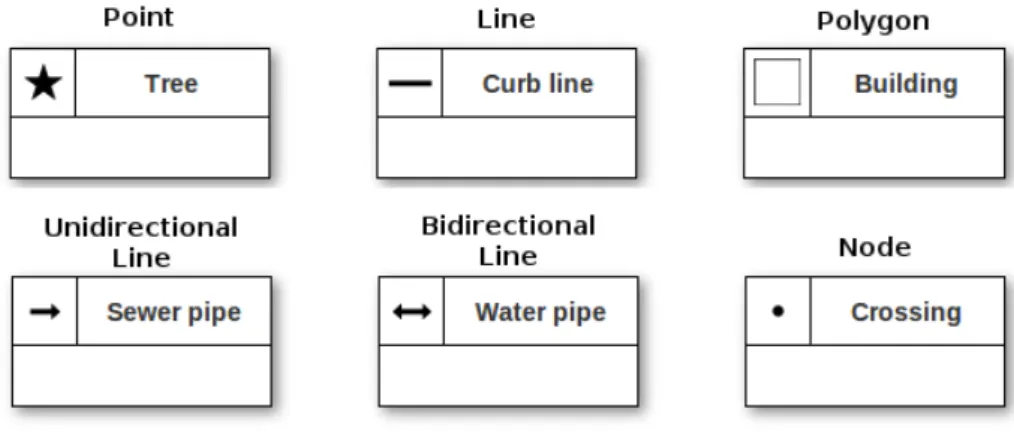
OMT-G specifies two types of classes in the class diagram: georeferenced and conven-tional. The georeferenced class notation have a top left-hand rectangle that points the geometry of the representation, whereas the notation used for conventional classes is similar to the notation used in the UML [Booch et al., 2005], as it is shown in Figure 3.1.
Figure 3.1: Simplified graphical notation of a class in OMT-G.
3.1. Class diagram 19
and bidirectional arcs). Geo-fields correspond to variables such as soil type, relief and temperature, often seen as a surface, and can be represented by isolines, tesselation, planar subdivision, sampling or triangular irregular network (TIN). Figures 3.2 and 3.3 show, respectively, examples of geo-object and geo-field classes.
Figure 3.2: Geo-object classes
Figure 3.3: Geo-field classes
3.1.2
Relationships
OMT-G represents three basic types of relationships that can occur between its classes: simple associations,network relationships and spatial relationships, along with object-oriented relationships (generalization/specialization, aggregation andconceptual gener-alization).
ob-20 Chapter 3. The OMT-G Model
nected objects. This type of relationship only shows the need for a logical connection, not a requirement for the implementation of a particular structure. A sewage arc-node network is an example of this type of relation. The arcs represent the piping segments while the nodes are used to represent network elements such as manhole, sewage treat-ment station and discharge. Spatial relations represent the topological, metric, ordinal and fuzzy relationships. Some relationships, like topological, can be derived automat-ically from the geometry of each object during the execution of data entry or spatial analysis operations. Others, called explicit relationships, need to be specified by the user in order to allow the system to store and maintain that information. OMT-G con-siders a set of nine different spatial relationships between georeferenced classes: touch, in,cross, overlap, disjoint,adjacent to,coincide, contain and near.
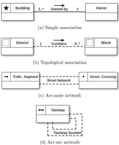
OMT-G makes it simple to distinguish between simple associations, spatial and network relationships. Simple associations are represented by continuous lines, whereas spatial relationships are indicated by dashed lines. Both relationships are characterized by their cardinality. The notation for cardinality adopted by OMT-G is the same used by UML. The network relationships are indicated by two parallel dashed lines, linking a node class to an arc class. Network structures without nodes can be indicated by a recursive relationship on the class which represents graph segments. The name given to the network is annotated between the two dashed lines. Figure 3.4 shows the OMT-G notations for relationships.
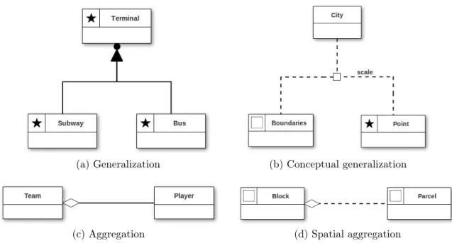
Generalization and specialization relationships present similar behavior to con-ventional object-oriented hierarchies. They apply to both georeferenced and conven-tional classes, following the definitions and notation proposed for UML (Figure 3.5a), where a triangle connects a superclass to its subclasses. Generalizations can be speci-fied astotal orpartial. A generalization is total when the union of all instances of the subclasses is equivalent to the complete set of instances of the superclass. They can also bedisjoint oroverlapping. In a disjoint generalization/specialization, an instance must belong to at most one subclass.
3.2. Integrity Constraints 21
(a) Simple association
(b) Topological association
(c) Arc-node network
(d) Arc-arc network
Figure 3.4: OMT-G notations for relationships.
Aggregation is a special form of association between objects, where one of them is considered to be congregated from others. The graphic notation used in OMT-G follows the one used in UML (Figure 3.5c). An aggregation can occur between conventional classes, georeferenced classes and georeferenced and conventional classes. In the latter case, a spatial aggregation (i.e. “whole-part” aggregations) must be used (Figure 3.5d).
3.2
Integrity Constraints
22 Chapter 3. The OMT-G Model
(a) Generalization (b) Conceptual generalization
(c) Aggregation (d) Spatial aggregation Figure 3.5: OMT-G notations for generalizations and aggregations.
are also constraints which apply to the geometric representation of geo-objects (i.e., constraints related to the consistency of points, lines, polygons etc.).
3.2.1
Geo-field constraints
The spatial integrity rules (R1 – R5) can be deduced from the semantics involved in the concept of geo-fields and, also, from the specific definition of its four descendant classes. Particularly, all representations must correspond to the entire field being modeled, that is, it must be possible to infer a value at any point of the field of interest from the information contained in one of these representations.
(R1) Planar Enforcement Rule: Let F be a geo-field and let P be a point such that P ⊂ F. Then a value V(P) = f(P, F), i.e., the value of F at P, can be univocally determined.
(R2) Isoline: Let F be a geo-field. Let v0, v1, . . . , vn be n+ 1 points in the plane.
Let a0 = v0v1, a1 = v1v2, . . . , an−1 = vn−1vn be n segments, connecting the
points. These segments form an isoline L if, and only if, (1) the intersection of adjacent segments in L is only the extreme point shared by the segments (i.e., ai∩ai+1 =vi+1), (2) non-adjacent segments do not intercept (that is, ai∩aj =∅
3.2. Integrity Constraints 23
(R3) Tesselation: Let F be a geo-field. Let C = {c0, c1, c2, . . . , cn} be a set of
regularly-shaped cells covering F. C is a tesselation of F if and only if for any point P ⊂F, there is exactly one corresponding cellci ∈C and, for each cellci,
the value of F is given.
(R4) Planar Subdivision: LetA={A0, A1, A2, . . . , An}be a set of polygons and F
be a geo-field. Such that Ai ⊂F for all i such that0≤i≤n. A forms a planar
subdivision representing F if and only if for any point P ⊂ F, there is exactly one corresponding polygon Ai ∈ A, for which a value of F is given (that is, the
polygons are non-overlapping and cover F entirely).
(R5) Triangular Irregular Network (TIN): Let F be a geo-field. Let T =
{T0, T1, T2, . . . , Tn} be a set of triangles such that Ti ⊂ F for all i such that
0≤i≤n. T forms an triangular irregular network representing F if and only if for any point P ⊂F, there is exactly one corresponding triangle Ti ∈T, and the value of F is known at all of vertices of Ti.
3.2.2
Geo-object constraints
The geometric concepts used in the definition of points, lines (including lines with a topological role), and polygons lead to some integrity constraints. In OMT-G it is admissible the existence of geo-objects that are formed by multiple polygons, establish-ing one of them as a base polygon and considerestablish-ing the others as holes. The followestablish-ing constraints (R6 – R8) are regarding lines and polygons.
(R6) Line: Let v0, v1, . . . , vn be n+ 1 points in the plane. Let a0 =v0v1, a1 =v1v2, . . . , an−1 = vn−1vn be n segments, connecting the points. These segments form
a polygonal line L if, and only if, (1) the intersection of adjacent segments in L is only the extreme point shared by the segments (i.e., ai ∩ai+1 = vi+1), (2) non-adjacent segments do not intercept (that is, ai∩aj =∅for all i, j such that j 6=i+ 1), and (3) v0 6=vn, that is, the polygonal line is not closed.
(R7) Simple Polygon: Let v0, v1, . . . , vn be n+ 1 points in the plane, with n > 3.
Let s0 = v0v1, s1 = v1v2, . . . , sn−1 = vn−1vn be a sequence of n−1 segments,
24 Chapter 3. The OMT-G Model
(R8) Polygonal Region: Let R = {P0, P1, ..., Pn−1} be a set formed by n simple
polygons in the plane, with n > 1. Considering P0 to be a basic polygon, R forms apolygonal region if, and only if, (1) polygonP0 has its vertices coded in a counterclockwise fashion, (2) Pi disjoint Pj for all Pi 6=P0 in which the vertices are coded counterclockwise, and (3) P0 contains Pi for all Pi 6=P0 in which the vertices are coded clockwise.
3.2.3
Network relationship constraints
Network relationships involve objects that are connected with each other. These rela-tionships only show the need for a logical connection, not requiring the implementation of any particular data structure. The connectivity rules, which apply to network rela-tionship primitives, are R9 and R10.
(R9) Arc-node network: LetG={N, A}be a network structure composed of a set of nodes N ={n0, n1, . . . , np}and a set of arcs A={a0, a1, . . . , aq}. Members of
N and members of A are related according to the following constraints:
1. For every nodeni ∈N there must be at least one arc ak ∈A.
2. For every arcak ∈A there must be exactly two nodes ni,nj ∈N.
(R10) Arc-arc network: Let G={A} be a network structure composed of a set of arcs A={a0, a1, . . . , aq}. Then the following constraint applies:
1. Every arc ak ∈ A must be related to at least one other arc ai ∈ A, where
k 6=i.
3.2.4
Spatial aggregation constraint
Aggregation is a special form of association between objects, where one of them is considered to be mounted from others and can occur between all types of classes. When the aggregation is between georeferenced classes, a spatial integrity constraint is imposed considering the existence of the aggregated object and its corresponding sub-objects. This constraint must verify that the geometry of the whole is fully covered by the geometry of the parts and that no overlapping among the parts occurs, as described in rule R11.
(R11) Spatial aggregation: LetP ={P0, P1, . . . , Pn} be a set of geo-objects. Then
3.2. Integrity Constraints 25
for all isuch that 0≤i≤n, and (2)(W ∩Sni=0Pi) =W, and (3) ((Pi touch Pj) ∨ (Pi disjoint Pj)) = TRUE for all i, j such thati6=j.
3.2.5
Spatial relationship constraints
Spatial relations represent direction, topological, metric, ordinal, and fuzzy relation-ships. Some relationships can be derived from the geometry of each object, during the execution of data insertion or spatial analysis operations. Others need to be speci-fied by the user, in order to allow the system to store and maintain that information. OMT-G considers a set of five basic spatial relationships between georeferenced classes, from which all others can be derived [Clementini et al., 1993; Davis Jr. et al., 2005]: crosses,disjoint, overlaps, touches and within.
The integrity constraints RT1 to RT5 consider these spatial relationships types. These constraints are formulated using a notation in which objects are indicated by upper-case italic letters (e.g., A, B), their boundaries are denoted as ∂A, and their interiors as A◦. The boundary of a point object is considered to be always empty
(therefore, the point is equivalent to its interior), and the boundary of a line is consisted of its two endpoints. A function, named dim, is used to return the dimension of an object and returns 0 if the object is a point, 1 if it is a line, or 2 if it is a polygon. Notice that some relationships are only allowed between specific classes because they depend on the geometric representation. For instance, the existence of a touches relationship assumes that none of the classes involved are a point.
(RT1) Crosses: Let A be a geo-object of the Line class, and let B be a geo-object of either the Line or the Polygon class. Then (A crosses B) = TRUE ⇔
dim(A◦∩B◦) =(max(dim(A◦), dim(B◦))-1) ∧(A∩B 6=A)∧(A∩B 6=B).
(RT2) Disjoint: Let A and B be two geo-objects. Then (A disjoint B) = TRUE
⇔A∩B =∅.
(RT3) Overlaps: Let A and B be two geo-objects. Both members of the Line or of the Polygon class. Then (A overlaps B) = TRUE ⇔ dim(A◦) = dim(B◦) =
dim(A◦∩B◦) ∧(A∩B =6 A)∧(A∩B 6=B).
(RT4) Touches: Let A and B be two geo-objects, where neither A nor B are mem-bers of the Point class. Then (A touches B) = TRUE ⇔ (A◦∩B◦ = 0) ∧
(A∩B 6=∅).
26 Chapter 3. The OMT-G Model
OMT-G considers, for convenience, a larger set of spatial relationships con-straints, due to cultural or semantic concepts that are familiar to the users. These constraints (RT6 to RT13) are special cases of one of the five basic relationships, but they deserve a special treatment because of their common use in practice. Constraints RT12 and RT13 represent metric relationships and require a parameter, since the no-tion of proximity varies according to the situano-tion, a precise distance must be supplied in order to allow the correct evaluation of the relationship.
(RT6) Equals: Let A and B be two geo-objects. Then (A equals B) = TRUE ⇔
A∩B =A=B.
(RT7) Contains: Let A and B be two geo-objects, where A is a member of the
Polygon class. Then (A contains B) = TRUE ⇔ ((B within A) = TRUE) ∧
((A equals B) = FALSE).
(RT8) ContainsProperly: Let A and B be two geo-objects, where A is a member of the Polygon class. Then (A containsproperly B) = TRUE ⇔ ((B within A) = TRUE) ∧ ((A touches B) = FALSE).
(RT9) Covers: Let A and B be two geo-objects. Then (A covers B) = TRUE ⇔
A∩B =A.
(RT10) CoveredBy: LetA andB be two geo-objects. Then (A covers B) = TRUE
⇔ A∩B =B.
(RT11) Intersects: LetAandB be two geo-objects. Then (Aintersects B) = TRUE
⇔ ((A disjointB) = FALSE).
(RT12) Distant(dist): Let A and B be two geo-objects. Let C be a buffer, created at a distance dist around A. Then (A distant(dist) B) = TRUE ⇔ (B disjoint C) = TRUE.
3.3. Mapping OMT-G to object-relational spatial databases 27
Table 3.1: Geometric types: OMT-G and OGC SFS
OMT-G representation OGC SFS representation
Point Point
Line LineString
Polygon MultiPolygon
Node Point
Unidirectional Arc LineString Bidirectional Arc LineString
Isolines LineString
Sample Point
Planar Subdivision Polygon or Multipolygon
Triangular Irregular Network Point (vertices) and Polygon (triangles)
Tesselation –
3.3
Mapping OMT-G to object-relational spatial
databases
Geometric types in conceptual schemas are accompanied by an expected behavior, captured with a set of spatial integrity constraints [Borges et al., 2002]. Geo-objects, for example, like lines, arcs and polygons must be formed by simple lines or simple polygonal lines, that is, lines without self intersection or self tangency. Geo-fields, like sampling,tesselation,planar-subdivision,isoline andtriangular irregular network must be continuously distributed over the space, without overlapping between adjacent lines or polygons.
In contrast, the data types implemented by most modern spatial RDBMS are simple geometry types and geometry collections hierarchized by OGC. When mapping a spatial data model from the conceptual to the physical schema, we are forced to use these simple geometric representations available in the spatial RDBMS. This pro-cess implies in loss of semantics, since the only topological constraints implemented in the spatial RDBMS are simple value checks (e.g. a polygon is a closed line). Such constraints can ensure the geometric consistency of objects represented by lines or poly-gons. However, ensuring the consistency of aggregations or arc-node relationships, for example, is more complicated, usually requiring the development of triggers. This im-plementation, however, is not trivial and demands advanced knowledge of the resources offered by the RDBMS.
repre-28 Chapter 3. The OMT-G Model
and isolines. They have completely different behavior in the conceptual model, but they are all mapped tolinestring in the physical schema.
3.4
Further work on OMT-G
OMT-G motivated many initiatives, including Wispy [Fatto et al., 2015], a uDig1
exten-sion that permits verifying and visually specifying complex spatial integrity constraints. WiSPY includes a visual environment for defining spatial data models with integrity constraints and for automatically generating the constraint checker. The latter is used to verify the integrity of the data produced during the map editing process.
In an earlier work, Borges et al. [2005] inaugurate the study of spatial integrity constraints from OMT-G schemas, and propose an algorithm that allows for the map-ping between an OMT-G class diagram and an object-relational schema, which includes basic geometric representations as part of relations, along with conventional attributes. A list of conventional and spatial integrity constraints is also obtained. From the object-relational schema, a physical schema for spatially extended relational databases is easily derived, but spatial integrity constraints must be implemented using triggers, checks and assertions.
Hora et al. [2010] later implemented an OMT-G mapping tool to generate Oracle PL/SQL schemas2
, that includes triggers and procedures, and XML schemas3
. In [Hora et al., 2011], they proposed a methodology and an algorithm to map arcs and nodes, organized in a network using spatial relationships, from a OMT-G schema to a GML document.
Lizardo and Davis Jr. [2014] presented the OMT-G Designer4
, a web-based mod-eling tool for OMT-G that includes Hora et al.’s mapping algorithms. In this work, we extend OMT-G Designer with an alternative mapping algorithm for PostgreSQL/-PostGIS, that includes the spatial integrity constraints and advanced spatial data types introduced by AST-PostGIS.
Finally, Seufitelli et al. [2015] identified the challenges in mapping OMT-G prim-itives for non-relational paradigms in order to integrate relational and non-relational databases, creating a hybrid approach.
1 uDig: http://udig.refractions.net/ 2 OMTG2SQL: https://github.com/lab-csx-ufmg/omtg2sql 3 OMTG2GML: https://github.com/lab-csx-ufmg/omtg2gml 4
Chapter 4
AST-PostGIS
In this work, we propose AST-PostGIS (Advanced Spatial Types for PostGIS), an open-source SQL extension that implements conceptual design semantics for spatial relational database management systems. Written in PL/pgSQL1
, AST-PostGIS is currently available for PostgreSQL version 9.5 or superior and requires the spatial module PostGIS, version 2.0 or above. Like any other PostgreSQL extension, AST-PostGIS is easy to install and can be individually enabled in each database schema. During installation, the extension creates several new data types, functions, procedures and a table. In order to discern these extension objects from those already implemented in PostgreSQL and PostGIS, AST-PostGIS adopts as a standard theadvanced spatial type (AST) prefix for all names.
AST-PostGIS is intended to bridge the gap between the conceptual design and the physical implementation of spatial databases. By introducing advanced spatial data types, AST-PostGIS allows creating geographic columns on tables with behav-ior control, respecting the semantics for geo-objects and geo-field geometries defined by OMT-G. By installing trigger procedures to assert the consistency of spatial rela-tionships during data updates, AST-PostGIS permits making explicit roles for spatial relations, as, for example, network connectivity. Furthermore, by providing functions to verify the consistency of the database before enforcing relationships constraints, the extension allows to sanitize the data input in bulk. Those functions manage all the necessary information to identify inconsistent data, and indicate constraint violations in a log table.
The following three sections explain, in detail, each of these three features intro-duced by AST-PostGIS.
1
30 Chapter 4. AST-PostGIS
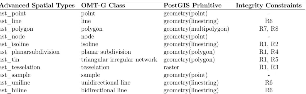
Table 4.1: Advanced spatial data types supported by AST-PostGIS
Advanced Spatial Types OMT-G Class PostGIS Primitive Integrity Constraints
ast_point point geometry(point)
-ast_line line geometry(linestring) R6
ast_polygon polygon geometry(multipolygon) R7, R8
ast_node node geometry(point)
-ast_isoline isoline geometry(linestring) R1, R2
ast_planarsubdivision planar subdivision geometry(polygon) R1, R4 ast_tin triangular irregular network geometry(polygon) R1, R5
ast_tesselation tesselation raster R1, R3
ast_sample sample geometry(point)
-ast_uniline unidirectional line geometry(linestring) R6 ast_biline bidirectional line geometry(linestring) R6
4.1
Advanced Spatial Data Types
Advanced Spatial Data Types are essentially the primitive geometric types of PostGIS coupled with a set of spatial integrity constraints to control their behavior, as expected by the designer in the conceptual level. These new spatial data types can be handled in the same way primitive types are, as they can be employed as column definition of tables, as variables in PL/pgSQL scripts or as arguments of functions or stored proce-dures. They can also be stored, retrieved and updated with the geometry processing functions of PostGIS.
The AST-PostGIS extension implements 11 Advanced Spatial Data Types. They are derived from the concepts of geo-objects and geo-fields classes of the OMT-G model and their semantics are controlled by the integrity constraints R1 – R8, defined formally in Section 3.2. These integrity constraints were implemented in PL/pgSQL scripts and encapsulated in the extension. Table 4.1 lists the Advanced Spatial Data Types implemented in AST-PostGIS, along with their georeferenced classes of the OMT-G model from where they were derived, the PostGIS primitive types that correspond to their geometry, and the integrity constraints that control their behavior.
4.2
Integrity constraints for spatial relationships
4.2. Integrity constraints for spatial relationships 31
In PostgreSQL, a trigger is associated with only one table and it executes a procedure when a certain event occurs in this table. Events can be either an insert, an update or a delete operation. Triggers can be specified to fire before events are attempted orafterthe events have been completed. In the latter situation, the state of the database is evaluated after the event completion and, in case the trigger constraints are violated, an exception is raised and a rollback operation is performed. If a trigger is marked for each row, it is called once for every row that the operation modifies, but a trigger that is marked for each statement, only executes once for any given operation, regardless of how many rows it modifies.
To implement integrity constraints on spatial relationships, AST-PostGIS re-quires that a trigger execute one of the custom procedures and be configured to fire
after an event occur and be marked with for each statement. The table associated with the trigger must also be one of the tables involved in the relationship. In case of a spatial aggregation relationship, the table associated must be the one that represents the part of the relationship. For arc-node relationships, the associated table can be either the arc or the node of the relationship. If it is the arc, the trigger blocks arc insertions or updates if there are no two nodes connected to them. If the associated table is a node, the trigger blocks nodes not connected to any arc. Spatial relationship triggers can also be associated to both tables of the relationship, but the choice of the table changes how the constraints are applied to the relationship.
The type of the operation must also be chosen according to the relationship on which the trigger is being applied. Arc-node networks and spatial relationships re-quire the trigger to fire afterinsertand updateoperations, while spatial aggregations demand all three operations (insert, update and delete).
Besides having the name of the table associated directly with the trigger, the names of both tables must also be passed to the procedure as a parameter. Although this requirement is a bit redundant, it is necessary for the trigger to identify which is the other table involved in the relationship. Furthermore, as feature tables can have multiple geometric columns, the name of these columns, associated in the relationships, must be passed to the procedure to avoid ambiguity. The order of the parameters is also important. For example, spatial aggregation trigger requires the part table name to be passed as the first parameter along with its geometric column name as the second parameter. Followed by the whole table name, as third parameter, and its the geometric column name, as fourth parameter. Listing 4.1 shows how a trigger for a spatial aggregation can be created.
32 Chapter 4. AST-PostGIS
CREATE TRIGGER t r i g g e r _ n a m e
AFTER INSERT OR UPDATE OR DELETE ON part_tbl
FOR EACH S TA TE ME N T EXECUTE P R OC ED UR E a s t _ a g g r e g a t i o n (
' part_tbl ' , ' part_geom ' , ' whole_tbl ' , ' whole_geom ' );
Listing 4.1: Aggregation Trigger
CREATE TRIGGER t r i g g e r _ n a m e AFTER INSERT OR UPDATE ON [ arc_tbl | node_tbl ]
FOR EACH S TA TE ME N T EXECUTE P R OC ED UR E a s t _ a r c n o d e n e t w o r k (
' arc_tbl ' , ' arc_geom ' , ' node_tbl ' , ' node_geom ' );
Listing 4.2: Arc-Node Trigger
parameters, which are (1) the name of arc table, (2) the name of geometric column (must be of typeast_uniline orast_biline), (3) the name of table representing a node, and (4) the name of the column of the node geometry, whose type is ast_node. The configuration of a trigger and its procedure to a arc-node network is illustrated in Listing 4.2. When the procedure is used with an arc-arc network relationship, only two parameters are accepted, which are (1) the arc table’s name and (2) its geometric column.
AST-PostGIS considers a set of 12 different spatial relationships between two georeferenced classes. What differentiates one type of relationship from another is the relationship operator passed to the trigger procedure.
AST-PostGIS supports the minimum set of spatial relationship operators, iden-tified by Clementini et al. [1993] and adopted by OMT-G [Davis Jr. et al., 2005], from which all others can be specified: Crosses, Disjoint, Overlaps, Touches and
4.2. Integrity constraints for spatial relationships 33
CREATE TRIGGER t r i g g e r _ n a m e AFTER INSERT OR UPDATE ON a_table
FOR EACH S TA TE M EN T EXECUTE PR OC ED UR E a s t _ s p a t i a l r e l a t i o n s h i p (
' a_table ' , ' a_geom ' , ' b_table ' , ' b_geom ' ,
' s p a t i a l _ r e l a t i o n s h i p ' , <' distance ' > );
Listing 4.3: Spatial Relationship Trigger
spatial relationships are admitted: Distant and Near. These require as a parameter the value of the distance in which the relationship occurs.
The parameters passed to ast_spatialrelationship are: (1) table A name, (2) geometry A name, (3) table B name, (4) geometry B name, and (5) spatial relationship operator. When the spatial relationship is Distant or Near, a sixth parameter is admitted with the value of the distance. Listing 4.3 illustrates the trigger configuration for a topological relationship. This trigger requires to be associated to table A, whose name is passed as a parameter after the statement ON.
In PostgreSQL, triggers are only fired if an event ensues on the table to which they are associated. A problem arises when users alter the other table of the relationship, if there is no trigger on that table to catch the event. This operation can lead the spatial relationship to an inconsistent state. For instance, consider an arc-node relationship on which the trigger was created associated to the arc table. This trigger ensures that every arc instance, stored in the table, is connected to two nodes from the node table. However, if a user deletes a node on the node table connected to an arc, no trigger would catch and block this operation, leaving an arc connected to only one node. This situation violates rule R9, defined in Section 3.2.
34 Chapter 4. AST-PostGIS
Table 4.2: Consistency check functions supported by AST-PostGIS
Spatial relationship Consistency check function
Spatial Relationship
ast_isSpatialRelationshipValid (a_tbltext, a_geom text, b_tbltext, b_geom text, relationship text)
ast_isSpatialRelationshipValid (a_tbltext, a_geom text, b_tbltext, b_geom text, relationship text, distreal)
Arc-Node Network ast_isNetworkValid (arc_tbltext, arc_geom text, node_tbltext, node_geom text)
Arc-Arc Network ast_isNetworkValid (arc_tbltext, arc_geom text)
Spatial Aggregation ast_isSpatialAggregationValid (part_tbltext, part_geomtext, whole_tbltext, whole_geom text)
SELECT a s t _ i s N e t w o r k V a l i d ( a r gu me nt s );
Listing 4.4: Usage of the consistency check function for network relationship
4.3
Consistency Check Functions
The spatial integrity constraints introduced in the previous subsection have to be ap-plied when a database is created and before any data is stored. They work by checking data operation events (like insertions, updates and deletions) when they occur. To ver-ify a non empty spatial database for violations on spatial relationships, AST-PostGIS provides consistency check functions, as shown in Table 4.2. These functions can be called before the initial enforcement of constraints, and they not only inform if the spatial relationship is invalid, but also identify the geometries that cause the violation.
The consistency check functions are not executed by triggers. Instead, they are called by a straightforward SELECT statement, omitting the FROM clause as shown in Listing 4.4. Just like the trigger procedures described in last subsection, consistent check functions also require parameters, which are the same as in the procedures.
4.4. Summary of limitations 35
Figure 4.1: AST-PostGIS log table schema
4.4
Summary of limitations
AST-PostGIS has three known limitations, mostly due to the way spatial representa-tions and relarepresenta-tionships are implemented in a RDBMS extension.
First, the triggers that create integrity constraints for relationships require a rigid statement structure in their creation. The triggers must be specified with different statements for each relationship type, as explained in Section 4.2. This is necessary to overcome the limitations imposed by PostgreSQL/PostGIS in the support for spatial concepts. It would be simpler, instead, if integrity constraints for spatial relationships, networks and aggregations could be specified using the DDL, analogously to the FOR-EIGN KEY statement for referential integrity in SQL, with the necessary verifications included in the DBMS’s code. In order to overcome this problem, AST-PostGIS runs scripts to check if the trigger statements are correct during their creation processes, and raises clarifying exceptions if not.
The trigger procedures, introduced by our extension to add integrity constrains on spatial relationships, receive as parameters not only the names of the feature ta-bles involved in the relationship, but also the names of their corresponding geometric columns. These parameters are required to avoid ambiguity problems when feature tables have multiple georeferenced columns, although in most cases there is only one geometric column per table. Using the geometry_columns view in PostGIS does not resolve this problem.