Abstract
Several researchers have studied suicide seasonality through different statistical approaches. In the present research, we performed a detailed statistical study of Brazilian suicide data registered from 1980 to 2010 using a new approach known as Threshold Bias Model (TBM). Eleven-year cyclic oscillations were observed in suicide rates that, at first sight, appear as being negatively correlated with the cycles of solar activity. Such oscillations are more noticeable for males although they also have been observed in the female rates.
Keywords: suicide; seasonal variations; solar activity.
Resumo
Vários pesquisadores têm estudado a sazonalidade do suicídio utilizando diversas abordagens estatísticas. Na presente pes-quisa, realizamos um estudo estatístico dos dados de suicídio brasileiros registrados entre 1980 e 2010 utilizando uma nova abordagem conhecida como Modelo da Tendência Limiar (TBM). Foram observadas oscilações com período de 11 anos nas taxas de suicídio que, à primeira vista, parecem ser negativamente correlacionadas com os ciclos de atividade solar. Essas os-cilações foram mais notáveis nas taxas masculinas, ainda que também tenham sido observadas nas taxas femininas.
Palavras-chave: suicídio; variações sazonais; atividade solar.
Suicide seasonality: Evidence of 11-year
cyclic oscillations in Brazilian suicide rates
Sazonalidade do suicídio: Indícios de oscilações cíclicas
de 11 anos nas taxas de suicídio brasileiras
Walter Sydney Dutra Folly
1Study carried out at Universidade Federal de Sergipe (UFS) – Itabaiana (SE), Brasil.
1DSc, Adjunct Professor and Researcher at Núcleo Integrado de Pesquisa e Pós-Graduação em Educação e Ciências (NIPPEC), UFSE – Itabaiana (SE), Brasil.
Mailing address: Walter Sydney Dutra Folly – Avenida Vereador Olímpio Grande, s/n – CEP: 49500-000 – Itabaiana (SE), Brazil – E-mail: [email protected] Financial support: none.
INTRODUCTION
Suicide seasonality is a multifactorial phenomenon that is oten associated with the increased winter-summer variation in the number of sunlight hours that occurs in temperate and polar zones of the globe1,2. Consequently, its occurrence has been little studied in the tropics.
In Brazil, a previous study conducted between 1996 and 2004 in the city of São Paulo (located on the Tropic of Capricorn) did not revealed significant correlation between suicides and the number of sunlight hours3. However, beyond the hypothetical influence of the daily duration of sunlight on suicide rates, several authors have reported that long-term seasonal patterns in such rates may be correlated with solar and geomagnetic activities4-7.
Since seasonal oscillations in suicide rates may be small in comparison with data luctuations due to death undercount-ing and/or cause of death misclassiication, researchers are using several statistical methods in order to quantify this phe-nomenon8,9. Considering this, we performed a preliminary study of suicide seasonality in Brazil employing the recent-ly proposed hreshold Bias Model (TBM)10 — a model that provides useful comparison parameters to help us identify seasonality patterns.
METHOD
he present research considers male and female suicide rates structured by age that were recorded in Brazil from 1980 to 2010. Such data are openly available from the website of DATASUS11. In the same way, the average sunspot numbers considered here (relating to solar cycles 21, 22 and 23) can be freely obtained from the website of the Solar Inluences Data Analysis Center (SIDC)12.
All analyses were made using the sotware Microcal Origin version 5.013. In this sotware, suicide rates were ed-ited in proper worksheets and plotted as functions of age. hen, we employed the Levenberg-Marquardt method to it Equation 1 (TBM distribution) to these datasets consider-ing β=11 as discussed in Folly10. he meanings of all TBM parameters were explained in this reference.
(1)
SR(t) =
a. + b - V0 .Cap.
- a + V0 . (t - τ1/2) if (t ≥ tc)
if (t < tc)
β + 1
τ1/2 τ1/2
t - τ1/2 β
τ1/2
t - τ1/2
β + 1
0
.
exp
Ater all the distributions were itted, we used the values of the parameters b, V0 and Cap to calculate the middle-age suicide rates SR (τ1/2) for each year from 1980 to 2010 using the expression SR (τ1/2) = (b-V0).Cap. Such distributions were numerically integrated (using Origin’s integration tool) from the critical age tc to ininity in order to determine the areas under the curves. he values of tc can be calculated using Equation 2.
β + 1 τ1/2
tc = τ1/2 - τ1/2 (b - V0) a
1 β
1
(2)
he areas under the TBM distributions and the calculated values of SR (τ1/2) were plotted together with sunspot num-bers in a same time scale to facilitate comparisons. In order to quantify the period and amplitude of seasonal oscillations of these data, they were itted by the function f (T) deined by the Equation 3, in which T is the time in years. he year 1980 was considered as the zero on the time scale.
he Equation 3 deines f (T) as being the sum of a third order polynomial (necessary to it the secular trend) and a sinusoidal term in which the parameters P5, P6 and P7 are the amplitude, period in years and initial phase respectively.
P6
2πT f (T) = P1 + P2 . T + P3 . T2 + P
4 . T
3 + P
5 . sin + P7 (3)
RESULTS
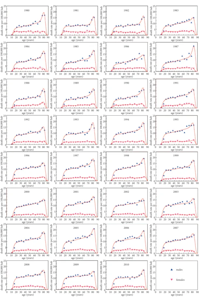
he TBM distributions were itted to yearly suicide rates by age from 1980 to 2010 (Figure 1). he obtained parameter values with standard errors, chi-squares, degrees of freedom and p-values are shown in the Table 1. Despite the distribu-tions itted better the female data, even for males, the dif-ferences between itting curves and statistical data were not signiicant (all p>0.05), with the worst it observed for the year 1987 (p=0.975).
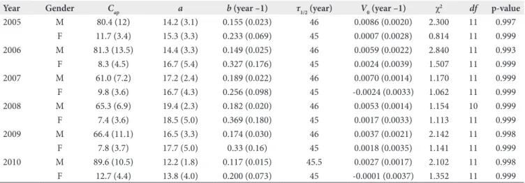
We organized the curves for the male datasets in a 3D graph in order to depict their annual evolution over the studied period (Figure 2). By performing numerical integra-tions, we determined the areas under the itted distributions for males and females. Such areas are shown in the Figure 3a with the sunspot numbers for solar cycles 21, 22 and 23 on the same time scale. In the same way, the calculated middle-age suicide rates SR (τ1/2) are shown together with sunspot data in Figure 3B.
Figure 1. Annual suicide rates by age and gender in Brazil from 1980 to 2010. The continuous curves shown in red are the Threshold Bias Model (TBM) distributions fitted to each statistical dataset
1980 1981 1982 1983
1984 1985 1986 1987
1988 1989 1990 1991
1992 1993 1994 1995
1996 1997 1998 1999
2000 2001 2002 2003
2004 2005 2006 2007
2008 2009 2010
m a l e s
f e m a l e s 25 20 15 10 5 0
0 10 20 30 40 50 60 70 80 90 a ge (years)
d ea th r at e p er 100, 000 h ab 25 20 15 10 5 0
0 10 20 30 40 50 60 70 80 90 age (years)
de
at
h ra
te p
er 100,000 h
ab 25 20 15 10 5 0
0 10 20 30 40 50 60 70 80 90 age (years)
de
at
h ra
te p
er 100,000 h
ab 25 20 15 10 5 0
0 10 20 30 40 50 60 70 80 90 age (years)
de
at
h ra
te p
er 100,000 h
ab 25 20 15 10 5 0
0 10 20 30 40 50 60 70 80 90 age (years)
de
at
h ra
te p
er 100,000 h
ab 25 20 15 10 5 0
0 10 20 30 40 50 60 70 80 90 age (years)
de
at
h ra
te p
er 100,000 h
ab 25 20 15 10 5 0
0 10 20 30 40 50 60 70 80 90 age (years)
de
at
h ra
te p
er 100,000 h
ab 25 20 15 10 5 0
0 10 20 30 40 50 60 70 80 90 age (years)
de
at
h ra
te p
er 100,000 h
ab 25 20 15 10 5 0
0 10 20 30 40 50 60 70 80 90 age (years)
de
at
h ra
te p
er 100,000 h
ab 25 20 15 10 5 0
0 10 20 30 40 50 60 70 80 90 age (years)
de
at
h ra
te p
er 100,000 h
ab 25 20 15 10 5 0
0 10 20 30 40 50 60 70 80 90 age (years)
de
at
h ra
te p
er 100,000 h
ab 25 20 15 10 5 0
0 10 20 30 40 50 60 70 80 90 age (years)
de
at
h ra
te p
er 100,000 h
ab 25 20 15 10 5 0
0 10 20 30 40 50 60 70 80 90 age (years)
de
at
h ra
te p
er 100,000 h
ab 25 20 15 10 5 0
0 10 20 30 40 50 60 70 80 90 age (years)
de
at
h ra
te p
er 100,000 h
ab 25 20 15 10 5 0
0 10 20 30 40 50 60 70 80 90 age (years)
de
at
h ra
te p
er 100,000 h
ab 25 20 15 10 5 0
0 10 20 30 40 50 60 70 80 90 age (years)
de
at
h ra
te p
er 100,000 h
ab 25 20 15 10 5 0
0 10 20 30 40 50 60 70 80 90 age (years)
de
at
h ra
te p
er 100,000 h
ab 25 20 15 10 5 0
0 10 20 30 40 50 60 70 80 90 age (years)
de
at
h ra
te p
er 100,000 h
ab 25 20 15 10 5 0
0 10 20 30 40 50 60 70 80 90 age (years)
de
at
h ra
te p
er 100,000 h
ab 25 20 15 10 5 0
0 10 20 30 40 50 60 70 80 90 age (years)
de
at
h ra
te p
er 100,000 h
ab 25 20 15 10 5 0
0 10 20 30 40 50 60 70 80 90 age (years)
de
at
h ra
te p
er 100,000 h
ab 25 20 15 10 5 0
0 10 20 30 40 50 60 70 80 90 age (years)
de
at
h ra
te p
er 100,000 h
ab 25 20 15 10 5 0
0 10 20 30 40 50 60 70 80 90 age (years)
de
at
h ra
te p
er 100,000 h
ab 25 20 15 10 5 0
0 10 20 30 40 50 60 70 80 90 age (years)
de
at
h ra
te p
er 100,000 h
ab 25 20 15 10 5 0
0 10 20 30 40 50 60 70 80 90 age (years)
de
at
h ra
te p
er 100,000 h
ab 25 20 15 10 5 0
0 10 20 30 40 50 60 70 80 90 age (years)
de
at
h ra
te p
er 100,000 h
ab 25 20 15 10 5 0
0 10 20 30 40 50 60 70 80 90 age (years)
de
at
h ra
te p
er 100,000 h
ab 25 20 15 10 5 0
0 10 20 30 40 50 60 70 80 90 age (years)
de
at
h ra
te p
er 100,000 h
ab 25 20 15 10 5 0
0 10 20 30 40 50 60 70 80 90 age (years)
de
at
h ra
te p
er 100,000 h
ab 25 20 15 10 5 0
0 10 20 30 40 50 60 70 80 90 age (years)
de
at
h ra
te p
er 100,000 h
ab 25 20 15 10 5 0
0 10 20 30 40 50 60 70 80 90 age (years)
de
at
h ra
te p
er 100,000 h
ab 25 20 15 10 5 0
0 10 20 30 40 50 60 70 80 90 age (years)
de
at
h ra
te p
er 100,000 h
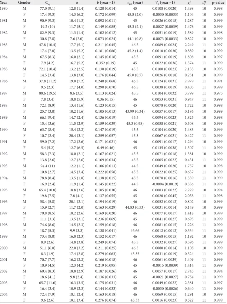
Year Gender Cap a b (year –1) τ1/2 (year) V0 (year –1) χ2 df p-value
1980 M 77.0 (9.1) 12.8 (1.4) 0.120 (0.014) 45 0.0108 (0.0020) 1.498 10 0.998
F 17.4 (9.3) 14.3 (6.2) 0.172 (0.099) 45.5 (2.0) -0.0030 (0.0033) 1.104 10 0.999
1981 M 90.9 (9.3) 10.4 (1.3) 0.092 (0.011) 45 0.0026 (0.0018) 1.287 10 0.999
F 19.2 (10) 11.7 (5.1) 0.149 (0.085) 45.3 (2.1) -0.0027 (0.0039) 1.476 10 0.999
1982 M 82.9 (9.3) 11.3 (1.4) 0.102 (0.012) 45 0.0051 (0.0019) 1.589 10 0.998
F 30.8 (7.8) 7.6 (2.0) 0.073 (0.024) 44.1 (0.8) -0.0073 (0.0033) 0.827 10 0.999
1983 M 47.8 (10.4) 17.7 (5.1) 0.211 (0.045) 46.5 0.0089 (0.0024) 2.249 11 0.997
F 17.4 (7.8) 13.5 (5.2) 0.181 (0.086) 45.2 (1.4) 0.0010 (0.0030) 0.889 10 0.999
1984 M 67.5 (8.3) 16.0 (2.1) 0.145 (0.018) 45.5 0.0091 (0.0019) 1.808 10 0.997
F 7.9 (4.2) 16.7 (5.2) 0.352 (0.19) 45 0.0022 (0.0036) 1.374 11 0.999
1985 M 72.1 (10.4) 13.2 (2.5) 0.130 (0.019) 45.5 0.0100 (0.0023) 2.133 10 0.995
F 14.5 (3.4) 13.8 (3.0) 0.176 (0.044) 45.0 (0.7) 0.0026 (0.0018) 0.231 10 0.999
1986 M 37.8 (11.2) 19.0 (7.2) 0.240 (0.068) 46.5 0.0124 (0.0031) 2.979 11 0.991
F 9.5 (2.3) 17.7 (4.0) 0.290 (0.070) 46.5 0.0038 (0.0019) 0.405 11 0.999
1987 M 88.6 (19.5) 8.6 (3.5) 0.113 (0.024) 45.5 0.0104 (0.0032) 3.799 11 0.975
F 7.8 (3.4) 18.8 (5.9) 0.36 (0.15) 46 0.0053 (0.0031) 0.947 11 0.999
1988 M 72.1 (8.9) 13.4 (1.6) 0.123 (0.015) 45 0.0078 (0.0020) 1.722 10 0.998
F 25.7 (3.0) 10.2 (1.6) 0.105 (0.013) 43.99 (0.34) 0.0057 (0.0017) 0.186 10 0.999
1989 M 66.1 (9.4) 14.7 (2.4) 0.136 (0.019) 45.5 0.0094 (0.0023) 1.825 10 0.998
F 15.4 (3.6) 11.5 (2.9) 0.159 (0.039) 45.3 (0.98) 0.0058 (0.0021) 0.308 10 0.999
1990 M 63.7 (8.4) 15.4 (2.2) 0.147 (0.019) 45.5 0.0104 (0.0020) 1.483 10 0.999
F 10.7 (2.4) 20.4 (3.1) 0.259 (0.057) 45.3 0.0067 (0.0021) 0.427 11 0.999
1991 M 59.0 (7.2) 17.2 (2.6) 0.171 (0.021) 46 0.0091 (0.0017) 1.294 10 0.999
F 5.4 (5.2) 12.7 (6.5) 0.49 (0.46) 45 0.0135 (0.0038) 1.307 11 0.999
1992 M 58.3 (7.3) 18.0 (2.1) 0.167 (0.021) 45.5 0.0071 (0.0018) 1.381 10 0.999
F 13.8 (2.6) 12.7 (2.6) 0.169 (0.034) 45.5 0.0005 (0.0022) 0.431 11 0.999
1993 M 94.4 (11) 12.2 (1.1) 0.106 (0.013) 44.5 0.0049 (0.0020) 1.757 10 0.998
F 10.8 (2.7) 14.5 (3.4) 0.222 (0.058) 45.5 0.0022 (0.0025) 0.637 11 0.999
1994 M 78.8 (8.4) 13.5 (1.8) 0.138 (0.015) 45.5 0.0078 (0.0016) 1.339 11 0.999
F 16.9 (2.4) 11.9 (1.4) 0.145 (0.022) 44.5 -0.0004 (0.0019) 0.336 11 0.999
1995 M 65.4 (10.8) 18.8 (3.6) 0.185 (0.030) 46 0.0083 (0.0022) 2.229 10 0.994
F 19.8 (7.5) 7.8 (4.1) 0.137 (0.055) 45 0.0020 (0.0045) 2.058 11 0.998
1996 M 58.4 (5.8) 20.1 (2.1) 0.194 (0.019) 46 0.0052 (0.0012) 0.802 10 0.999
F 15.9 (2.7) 11.7 (2.0) 0.163 (0.029) 44.83 (0.53) 0.0031 (0.0014) 0.149 10 0.999
1997 M 70.8 (8.5) 18.2 (2.6) 0.169 (0.020) 46 0.0077 (0.0017) 1.418 10 0.999
F 11.1 (3.3) 13.5 (3.1) 0.236 (0.069) 45 0.0041 (0.0027) 0.693 11 0.999
1998 M 74.6 (8.6) 14.5 (2.3) 0.159 (0.018) 46 0.0081 (0.0015) 1.226 11 0.999
F 18.7 (5.3) 9.9 (3.3) 0.138 (0.041) 46.66 0.0012 (0.0012) 0.334 11 0.999
1999 M 73.4 (8.0) 16.0 (2.3) 0.152 (0.017) 46 0.0068 (0.0015) 1.192 10 0.999
F 8.9 (2.6) 14.8 (3.8) 0.249 (0.074) 45.5 0.0032 (0.0027) 0.596 11 0.999
2000 M 51.1 (6.0) 22.0 (3.2) 0.211 (0.025) 46.5 0.0080 (0.0014) 1.108 10 0.999
F 8.3 (1.9) 17.4 (2.8) 0.279 (0.063) 45.35 0.0031 (0.0019) 0.324 11 0.999
2001 M 70.7 (7.7) 16.2 (2.2) 0.166 (0.018) 46 0.0061 (0.0039) 1.409 11 0.999
F 10.9 (4.5) 12.3 (4.2) 0.219 (0.095) 45 -0.0015 (0.0039) 1.414 11 0.999
2002 M 60.4 (8.3) 18.8 (2.9) 0.187 (0.026) 46 0.0057 (0.0017) 2.745 11 0.994
F 18.6 (4.1) 9.8 (2.4) 0.136 (0.033) 45 -0.0021 (0.0027) 0.754 11 0.999
2003 M 65.7 (11.6) 16.3 (3.5) 0.175 (0.031) 46 0.0049 (0.0022) 2.381 11 0.997
F 16.4 (3.4) 10.9 (2.3) 0.144 (0.033) 45 -0.0030 (0.0026) 0.640 11 0.999
2004 M 72.4 (7.9) 18.1 (2.4) 0.163 (0.018) 46 0.0069 (0.0015) 1.291 10 0.999
F 9.6 (2.6) 18.1 (3.4) 0.276 (0.074) 45.33 0.0016 (0.0023) 0.522 11 0.999
Table 1. Threshold Bias Model parameter values
Year Gender Cap a b (year –1) τ1/2 (year) V0 (year –1) χ2 df p-value
2005 M 80.4 (12) 14.2 (3.1) 0.155 (0.023) 46 0.0086 (0.0020) 2.300 11 0.997
F 11.7 (3.4) 15.3 (3.3) 0.233 (0.069) 45 0.0007 (0.0028) 0.814 11 0.999
2006 M 81.3 (13.5) 14.4 (3.3) 0.149 (0.025) 46 0.0059 (0.0022) 2.840 11 0.993
F 8.3 (4.5) 16.7 (5.4) 0.327 (0.176) 45 0.0024 (0.0039) 1.507 11 0.999
2007 M 61.0 (7.2) 17.2 (2.4) 0.189 (0.022) 46 0.0070 (0.0014) 1.170 11 0.999
F 9.8 (3.6) 16.7 (4.3) 0.256 (0.098) 45 -0.0024 (0.0033) 1.062 11 0.999
2008 M 65.3 (6.9) 19.4 (2.3) 0.182 (0.020) 46 0.0053 (0.0014) 1.154 10 0.999
F 7.4 (3.6) 18.5 (5.0) 0.369 (0.180) 45 0.0017 (0.0033) 1.113 11 0.999
2009 M 66.4 (11.1) 16.5 (3.3) 0.174 (0.030) 46 0.0037 (0.0021) 2.142 11 0.998
F 7.8 (3.7) 17.7 (5.0) 0.33 (0.16) 45 0.0018 (0.0035) 1.141 11 0.999
2010 M 89.6 (10.5) 12.2 (1.8) 0.117 (0.015) 45.5 0.0027 (0.0017) 2.102 11 0.998
F 12.7 (4.4) 13.8 (4.0) 0.200 (0.073) 45 -0.0001 (0.0037) 1.352 11 0.999
Table 1. Continuation
Figure 2. 3D representation of male Threshold Bias Model distributions plotted as functions of age and year. The continuous curve shown in red represents the annual evolution of middle-age death rates by suicide
1980 1985
1990 1995
2000 2005
2010
year
age (y ears)
0 20
40 60
80
deat h ra
te p er 100,000 h
ab
5 10
15 20
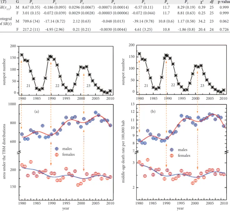
function f (T) defined by the Equation 3. The obtained pa-rameter values with respective standard errors, chi-squares, degrees of freedom and p-values are shown in Table 2. It was observed that the amplitude (modulus of parameter
P5 shown in Table 2) of the sinusoidal part of f (T) fitted to
SR (τ1/2) is about 6% of the average value of this quantity for males and 3% for females. In addition, it was found that the periods of the sinusoidal part of f (T) (values in years of P6
shown in Table 2) are closely compatible with the 11-year sunspot cycles. The Figures 3a and b show that the areas under the TBM distributions and the values of SR (τ1/2) present three events of minima in the studied time range: the first in 1979–1980, the second in 1989–1990 and the
third in 2001–2002. Such events occurred at approximately the same years of maxima of the sunspot cycles 21, 22 and 23 (Figures 3A and B).
DISCUSSION
Albeit some researchers have reported positive correlations be-tween suicide rates and sunspot numbers4, our preliminary results are in agreement with the i ndings of several other authors who have reported negative correlations between these phenomena5-7.
Since the middle-age suicide rates SR (τ1/2) and the areas under the TBM distributions are relatively immune to data l uctuations over the studied age groups, the results of present research can be considered as relatively robust.
Despite the observed oscillations in suicide rates be more prominent for males, they were also noticeable for females. For males, these oscillations are observed over all age groups, but become more intense with increasing ages (Figure 2). Such a progression with age was not clearly observed in the female rates. In Brazil, due to occupational factors, men are more likely to be exposed to sunlight than women14. h is fact may hypotheti-cally explain the greater amplitude of oscillations observed in the male suicide rates although this hypothesis has not been tested in the present study. h e reader should also be aware that the pres-ent results (obtained from nationwide population data) might not be valid at regional level. Interpretations of such results as being valid for small cohorts can lead to ecological fallacy15.
Table 2. Parameter values of f (T) obtained for SR(τ
1/2) and for integrated SR(t)
f (T) G P1 P2 P3 P4 P5 P6 P7 χ2 df p-value
SR(τ1/2) M 8.67 (0.35) -0.186 (0.093) 0.0296 (0.0067) -0.00071 (0.00014) -0.57 (0.11) 11.7 8.29 (0.19) 0.39 25 0.999
F 3.01 (0.15) -0.072 (0.039) 0.0029 (0.0028) -0.00003 (0.00006) -0.072 (0.044) 11.7 8.81 (0.63) 0.25 25 0.999
Integral
of SR(t) M 709.6 (34) -17.14 (8.72) 2.12 (0.63) -0.048 (0.013) -39.14 (9.78) 10.8 (0.6) 1.17 (0.58) 34.2 23 0.062
F 217.2 (11) -4.95 (2.96) 0.21 (0.21) -0.0030 (0.0044) 4.61 (3.25) 10.8 -1.86 (0.8) 20.4 24 0.726
Figure 3. Sunspot numbers during solar cycles 21, 22 and 23 plotted together with (A) the areas under Threshold Bias Model (TBM) distributions and (B) the middle-age death rates by suicide. The continuous curves shown in red and blue were obtained by fitting the function defined by the Equation 3 to these data for males and females respectively
200
sun
sp
o
t n
um
b
er
sun
sp
o
t n
um
b
er
150
100
50
0
ar
ea un
der t
h
e TBM di
st
ri
b
u
tio
n
s
21
1980
22 23
1985 1990 1995 2000 2005 2010
200
150
100
50
0 21
1980
22 23
1985 1990 1995 2000 2005 2010
1980 1985 1990 1995 2000 2005 2010 1000
800
600
200
150
males females
year
(a) (b)
males females
year
midd
le-a
ge de
at
h ra
te p
er 100,000 h
ab
13 12 11 10 9 8 7
3
2
1980 1985 1990 1995 2000 2005 2010
1. Lambert G, Reid C, Kaye D, Jennings G, Esler M. Increased suicide rate in the middle-aged and its association with hours of sunlight. Am J Psychiatry. 2003;160(4):793-5.
2. Björkstén KS, Kripke DF, Bjerregaard P. Accentuation of suicides but not homicides with rising latitudes of Greenland in the sunny months. BMC Psychiatry. 2009;9:20.
3. Nejar KA, Benseñor IM, Lotufo PA. Sunshine and suicide at the tropic of Capricorn, São Paulo, Brazil, 1996-2004. Rev Saude Publica. 2007;41(6):1062-64.
4. Dimitrov BD, Atanassova PA, Rachkova MI. Cyclicity of suicides may be modulates by internal or external 11-year cycles: An example of suicide rates in Finland. Sun and Geosphere. 2009;4(2):50-4.
REFERENCES
5. Stoupel E, Abramson E, Sulkes J, Martfel J, Stein N, Handelman M, Shimshoni M, Zadka P, Gabbay U. Relationship between suicide and myocardial infarction with regard to changing physical environmental conditions. Int J Biometeorol. 1995;38(4):199-203.
6. Túnyi I, Tesarová O. [Suicide and geomagnetic activity]. Soud Lek. 1991; 36(1-2):1-11.
7. Stoupel E, Petrauskiene J, Kalediene R, Abramson E, Sulkes J. Clinical cosmobiology: h e Lithuanian study 1990-1992. Int J Biometeorol. 1995;38(4):204-8.
9. Nader IW, Pietschnig J, Niederkrotenthaler T, Kapusta ND, Sonneck G, Voracek M. Suicide seasonality: Complex demodulation as a novel approach in epidemiologic Analysis. PLOS ONE. 2011;6(2):e17413.
10. Folly WSD. he hreshold Bias Model: A mathematical model for the nomothetic approach of suicide. PLOS ONE. 2011;6(9):e24414.
11. DATASUS – Informações de saúde [database on the Internet]. Brasil: Ministério da Saúde. 2011 [cited 2012 May 7]. Available from: http://tabnet.datasus.gov.br/cgi/deftohtm.exe?sim/ cnv/obt10uf.def Portuguese.
12. SIDC – Solar Inluences Data Analysis Center [Internet]. Brussels: Royal Observatory of Belgium. 2011 [cited 2012 May 2]. Available from: http:// sidc.be/sunspot-index-graphics/sidc_graphics.php
13. Microcal Origin [computer program]. Version 5.0. Northampton (MA): Microcal Sotware Inc.
14. Szklo AS, Almeida LM, Figueiredo V, Lozana VER, Mendonça GAS, Moura L, et al. Comportamento relativo à exposição e proteção solar na população de 15 anos ou mais de 15 capitais brasileiras e Distrito Federal, 2002-2003. Cad Saude Publica. 2007;23(4):823-34.
15. Robinson W S. Ecological correlations and the behavior of individuals. Am Sociol Ver. 1950;15(3):351-7.
16. Havaki-Kontaxaki BJ, Papalias E, Kontaxaki M-EV, Papadimitriou GN. Seasonality, suicidality and melatonin. Psychiatriki. 2010;21(4):324-31.