Cognitive Assessment of Topological Movement
Patterns and Direction turns: An Influence of Scale
Thesis
Master of Science in Geospatial Technologies
Farah Saeed
Institute for Geoinformatics University of M¨unster, Germany
Cognitive Assessment of Topological Movement Patterns
and Direction turns: An Influence of Scale
Farah Saeed
Thesis submitted to the Institute for Geoinformatics, University of
M¨
unster in partial fulfillment of the requirements for the degree of
Masters of Science in Geospatial Technologies.
Course Title:
Geospatial Technologies
Level:
Master of Science (M.Sc.)
Course Duration:
September 2009 - March 2011
Consortium:
University of M¨
unster (Germany)
Universitat Jaume I (Spain)
Universidade Nova de Lisboa (Portugal)
Supervisor:
Prof. Dr. Angela Schwering (ifgi, M¨
unster)
Co-Supervisor:
Prof. Dr. Alexander Klippel (PSU U.S.A)
Prof. Dr. Laura Diaz (UJI, Spain)
Contents
1 Introduction 1
1.1 Background . . . 2
1.2 Motivation . . . 3
1.3 Basic Concept of Spatial relation . . . 4
1.4 Basic Conception of spaces . . . 5
1.5 Research Questions and Hypothesis . . . 5
1.6 Structure of thesis . . . 6
2 Literature Review 7 2.1 Spatial Relation . . . 7
2.1.1 Topological Models . . . 8
2.1.2 Directional Models . . . 12
2.2 Mental Representation of spatial language . . . 15
2.3 Scale of spaces . . . 17
3 Methodology 19 3.1 Experiments . . . 19
3.2 Experiment 1 . . . 20
3.2.1 Experiment Material (Task 1) . . . 20
3.2.2 Experiment Material (Task 2) . . . 22
3.2.3 Experiment Procedure . . . 23
3.3 Experiment 2 . . . 25
3.3.1 Experiment Materials (Task One) . . . 26
3.3.3 Experiment Procedure . . . 27
4 Results and Discussion 29 4.1 Results of Experiment 1 . . . 29
4.1.1 Participants . . . 29
4.1.2 Task one . . . 30
4.1.3 Task Two . . . 35
4.2 Results of Experiment 2 . . . 39
4.2.1 Participants . . . 39
4.2.2 Task one . . . 39
4.2.3 Task two . . . 43
4.3 General Discussion . . . 45
5 Conclusion 48 5.1 Research Findings . . . 48
5.2 Future Work . . . 49
List of Figures
2.1 9-Intersection topological relationships . . . 9
2.2 RCC 8 Relationship . . . 9
2.3 26 topological DLine-region relations, together with the patterns of the corresponding 9+-intersection matrices . . . 11
2.4 A conceptual neighborhood graph of the 26 topological DLine-regions 11 2.5 Conceptual Neighborhood graph ( Source: Klippel, 2009) . . . 12
2.6 Cone based directional model . . . 13
2.7 Projection based directional model . . . 13
2.8 Triangular based model . . . 14
2.9 Enhanced triangular based model . . . 14
2.10 Direction relation matrix model . . . 15
3.1 Experiments Methodology Flowchart . . . 20
3.2 one path of the animated icon . . . 21
3.3 Examples of different position of bike passing through the city . . . 22
3.4 Depiction of the direction terminology Source:(Klippel and Montello, 2007) . . . 23
3.5 Instructions given for the experiment . . . 24
3.6 Screenshot of the window which participant saw initially in experi-ment 1 . . . 25
3.7 Example of different position of bike passing through the park . . . 26
4.1 Cluster Analysis using Average linkage method for task 1of
Experi-ment 1 . . . 31
4.2 Cluster Analysis using ward’s method for task 1of Experiment 1 . . 31
4.3 Euclidean distance model . . . 34
4.4 Cluster Analysis using Single linkage method for task 2 of Experi-ment 1 . . . 37
4.5 Cluster Analysis using Average linkage method for task 2 of Exper-iment 1 . . . 37
4.6 Cluster Analysis using Ward’s method for task 2 of Experiment 1 . 38 4.7 Cluster Analysis using ward’s method for task 1 of Experiment 2 . . 41
4.8 Cluster Analysis using Average linkage method for task 1 of Exper-iment 2 . . . 41
4.9 Euclidean distance model for scale 2 . . . 42
4.10 Dendrogram generated using Single linkage method (Task 2 of Ex-periment 2) . . . 44
4.11 Dendrogram generated using Ward’s method (Task 2 of Experiment 2) . . . 44
4.12 Dendrogram generated using Average linkage method (Task 2 of Experiment 2) . . . 45
4.13 Direction Model . . . 47
A.1 Second path of bike (animated icon) passing through the city . . . . 57
A.2 Third path of bike (animated icon) passing through the city . . . . 57
A.3 9 Different position of bike (path 1) . . . 58
A.4 9 Different position of bike(path 3) . . . 58
A.5 Different direction paths of bike (Exp. 1, scale 1) . . . 59
A.6 Path 1 (bike passing through the park) . . . 59
A.7 Path 2 (bike passing through the park) . . . 60
A.8 Path 3 (bike passing through the park) . . . 60
A.9 Nine Different position of bike (path 1) . . . 63
List of Tables
Acknowledgements
I begin in the name of ALLAH, the most Beneficent, the most Merciful. Praise be to ALLAH, the Almighty, on WHOM ultimately we depend for sustenance and guidance. First and foremost I thank ALLAH for endowing me this opportunity and strength to complete my dissertation, after all the challenges and difficulties. My utmost gratitude is towards Prof. Dr. Angela Schwering for her supervision and contributions which made her a backbone of this research. Many thanks for her guidance, kind support, motivation, stimulating and constructive suggestions and discussions to bring the research into shape from the concept to the concluding stage of thesis. I could not have imagined having a better advisor and mentor for my thesis.
I would like to extend my thanks to my co-supervisors Prof Dr. Alexander Klippel and Prof Dr. Laura Diaz for their extremely valuable comments and useful sug-gestions.
Words fail me to express my appreciation to my fianc´e Muhammad Faraz Afzal, Research Assistant Doctorate student in Universit¨at Duisburg-Essen who sincerely devoted his precious time, assistance and steadfast encouragement for every ac-tivity. My appreciation also goes to his patience and sleepless nights to conduct the experiments and his help in each task. I also acknowledged for his effort and suggestions towards my progress in life.
I remain indebted to Hira Affan, Doctorate student in University of M¨unster for her great help and struggle to conduct the experiments of this research.
To my classmate Kunle ogundele for his kind help and support during the work of my thesis.
Dedication
This thesis is dedicated to my affectionate, loving and caring parents
Muhammad Saeed (Late) & Nighat Saeed
Who introduced me to joy of reading from my birth, Offered me unconditional love and support,
Declaration
I hereby declare that the submitted work has been completed by me the undersigned and I have not used any other than permitted reference sources or materials nor engaged in any plagiarism. All references and other sources used by me have been appropriately acknowledged in the work. I further declare that the work has not been submitted for the purpose of academic examination, either in its original or similar form, anywhere else.
FARAH SAEED
Institute f¨ur Geoinformatik University of M¨unster Germany
Abstract
information and deduce this information. It is also examined that cognitive classes constructed remain same in both scale. Furthermore, linguistic description is also evaluated in this research but not in much detail. Verbal labeling of the groups participant created also gives the idea about the human perception about the two different scales.
Chapter 1
Introduction
Object movements with respect to the area can have many spatial relations i.e.
The goal of this research is to how human beings distinguish and characterize different topological movement pattern and direction turns in their environment. The goal of this research is also focus to assess the influence of scale on the cognitive classes through human subject tests.
1.1
Background
Egenhofer (1991) define the topological relationship using the boundary, interior and exterior and describes that topological relations include disjoint/disconnect, equal, meet, inside, covered by, covers and overlap. Topological relationship de-lineates the existence of the relationship between the objects located in the space. The objects can be defined as the rivers, lakes, buildings, roads, parks etc. there are many topological relationships that exist in the space for example near, touch, overlap etc. in normal life and we describe relationships using natural language like hospital is near to my house, city main market is linked with the main road and canal etc. Freska (1992) introduced eight augmenting qualitative orientation relations namely right front, right neutral, right back, straight back, left back, left neutral and left front in human perception environment. Vorwerg & Rickheit (1998) also writes that the reference points constituting direction categories in-clude LEFT, RIGHT, IN-FRONT, BEHIND, ABOVE, and BELOW are related to physiologically anchor preferred directions in perception (p-212).
In cognitive science the study of the spatial relation and their use in human environ-ment has been a topic of interest for many years. All human beings use Qualitative spatial reasoning in their daily life to understand the spatial environment because information in the spatial environment is mostly available in the qualitative form.
basically related to the cognitive science, spatial relations and the use of spatial relations in natural language.
1.2
Motivation
Cognitive process is important for human behavior and is a fundamental part of human information processing. It gives familiarity about the approach and the way human beings use their knowledge. The relationship of the human beings representation of the objects and the spatial relations and expression is getting a very interesting topic in the cognitive sciences. This interest leads to the cogni-tive scientist to make the research that how the human beings conceptualize the representations of the objects and how they express this into the verbal information.
Topological relations are the most important spatial relation and comprise of only qualitative measures. Some important topological properties are disconnect, par-tial overlap, tangenpar-tial part, interior and exterior. These properties have gained the good place in cognitive science research because these properties are the essen-tial knowledge when people conceptualize the movement of the different objects. In recent years the spatial relation studies and natural language terms has also enhanced the attraction towards this concept.
Now a day we face a large number of spatial topological relations in our daily life. Human beings have good qualities to comprehend the dissimilarity of the qualitative spatial relations. People use natural language to describe these spatial relations. The question arises how the humans make spatial concepts about the objects and events in their minds and how they use these concepts in the natural language to systematize and communicate their ideas and to use those ideas in everyday life.
rea-soning work is also focused on the knowledge of direction and human beings use the angular directions in their daily life and express it into natural language. Many lo-cations of the things and places are usually described with respect to the important land marks, location of the known places and also using of the natural language explanation. Most of the location of the places or things is usually described by the verbal information and human beings derived information from these verbal description. People use the many directions terminologies in the normal daily life for example right, left, straight and back but still there are many other directions which are not often and easily conceptualize by the human beings in the normal life and are not often used for example at left 30◦ etc.
Various studies show that even though humans may perceive angular information precisely, in city street networks as well as in body and geographic spaces more generally, human conceptualize and remember it with limited precision (Klippel, 2009). This research also enhances and realizes the users to express the spatial relations in their natural language. Several different classes of scale exist in the environment. Small, medium and large scale environment has also an important influence on how human beings perceive, think and treat spatial information.
1.3
Basic Concept of Spatial relation
Topological relations describe the relationship between the objects (natural and unnatural) in the space. The canal is near to my house, John’s office is linked to the main road, this road finishes at the end of the metropolitan boundary are the example of the topological relations. Direction relation defines the situation /location of the objects with reference to a specific reference object. The man is in front of the post box is one of the example of the direction relation in which post box is a reference object.
1.4
Basic Conception of spaces
Montello writes in his paper ”scale and multiple psychologies of space” that scale has significant persuade on how human treats spatial information and several dis-tinct scale classes of space and he also defines the scale as ”ratio between the dimension of a representation and those of the things that it represents or in other words the relative size of the representation”. Hill define small scale space as space in which the whole area and everything can be seen from one vantage point and large scale space as a space where navigation or secondary sources e.g. maps are needed.
The examples of Large scale geographic space which is city, neighborhood, town, county or any other big and large area which is linked with roads, bridges and canals and cannot be seen with from a single visual perspective. On the contrary the room, house is the examples of the small scale geographic space which can be seen from one vantage point.
1.5
Research Questions and Hypothesis
• Do human beings distinguish different movement patterns?
For this thesis following hypothesis are selected.
Hypothesis 1: All movement patterns in the real world are distinguished on the basis of their topological characteristics.
Hypothesis 2: All moving entities in the surrounding environment depict differ-ent angular information.
Hypothesis 3: Different scale of spaces has an effect on the characterization of moving entities.
1.6
Structure of thesis
The thesis outline can be divided into five chapters. The first chapter gives a brief introduction, motivation, aim of the present research work. It also provides the basic idea about the spatial relations and human conception about the spaces. The remnant of the thesis is organized as follows.
Chapter 2
Literature Review
2.1
Spatial Relation
Spatial relations are regarded as one of the most unique aspects of spatial or ge-ographical information and have linked the space and natural language. Spatial relation defines the position of one object in space in reference to the other object. The secondary object can be termed as reference object. There are many factors involved in selecting a reference object such as size, mobility, stability, knowledge of listener, knowledge of speaker (Talmy 1983). Freeman (1975) presented a very early review on formal representation of the spatial relations. He proposed thirteen relations i.e left of, right of, beside (alongside, next to), above (over, higher than, on top of), below (under, underneath, lower than), behind (in back of), in front of, near (close to, next to), far, touching, between, inside (within) and outside. The visually perceived location is specified by perceived distance and direction (Loomis et al, 1996). Spatial expressions denote either distance or directional relations. Both types may combine in natural language use (schober, 1993).
are the examples of distance relations. On the contrary, in directional relations objects are located with respect to each other in terms of their relation to the observer. Direction relations depend on the position of the observer and because of the particular perspective they are also referred to Projective relations (Moore, 1976).
2.1.1
Topological Models
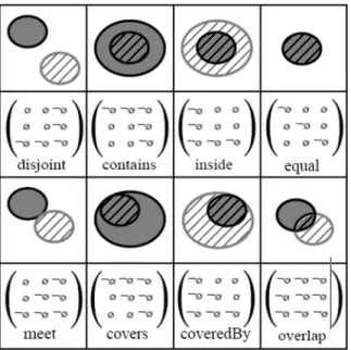
How two objects intersect with each other and what the relationship exist between the two objects is concerned with the topological relations. The study of topologi-cal relations has been studied for many decades in chase of spatial arrangements of the objects. Topological relations between spatial objects are the most important kind of qualitative spatial information (Li & Liu 2010). Topological relations are subset of geometric relations and do not include any quantitative measures only qualitative measures. Dozens of relation models have been proposed (Li & Liu 2010). These models usually make a small number of distinctions and therefore can only cope with spatial information at a fixed granularity of spatial knowledge (Li & Liu 2010). Topological relationship delineates the existence of the relation-ship between the objects located in the space. The objects can be defined as the rivers, lakes, buildings, roads, parks etc. there are many topological relationship that exist in the space for example near, far, touch, overlap etc. in normal life and we describe relationships using natural language like university is far from my house, city centre is near to my house. Egenhofer (1991) delineate the topologi-cal relationship using the interior, boundary and exterior and concluded the eight topological relations i.e disjoint/disconnect, equal, meet, inside, covered by, covers and overlap as shown in figure 2.1.
called RCC-8 relation (figure 2.2).
Figure 2.1: 9-Intersection topological relationships
Figure 2.2: RCC 8 Relationship
the one part of entity and the other part of the entity is empty or non-empty. The 9-intersection model discriminate eight spatial relations between the two simple connected regions with no holes and 33 relations between two simple lines and 19 spatial relations between a simple line and a simple region. Spatial entity could be one and two dimensional. For one dimensional entity such as lines the boundary consist of two end nodes and interior would be the every point exist on the line. In case of two dimensional entities such as region the definition of interior, exterior and boundary would be instinctive.
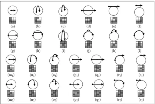
Kurata and Egenhofer (2007) proposed an extension of the 9-intersection called 9+-intersection model between the directed line segment and a region in a two dimensional space. This model structures the characteristics of the moving agent with respect to a region. This model made a distinction of the line’s boundary into two subparts i. e start and end point. The 9+-intersection distinguishes the 26 di-rected line region relationships as shown in figure 3. The conceptual neighborhood graph of the 26 directed Line region relations (Figure 2.3) is made and applied to the iconic depiction of movement patterns that satisfy a qualitative condition.
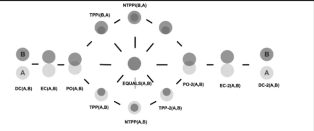
Figure 2.4 shows a conceptual neighborhood graph (Egenhofer and Al-Taha, 1992, Freska, 1992 ) of different movement patterns of two spatially extended entities. The concept of this neighborhood graph is based on Allen’s time interval (Allen, 1983). This graph employing the two frameworks for characterizing topological information i. e RCC-8 (Randell, Cui and Cohn, 1992) and 9-intersection model (Egenhofer, & Franzosa 1991).
Figure 2.3: 26 topological DLine-region relations, together with the patterns of the corresponding 9+-intersection matrices
similarity of the relation, the ward method and average complete linkage methods are used to yield similar clustering structure. According to the author different granularity levels exists in the topological relation conceptualization so the author proposed to use weights by using weight fusion coefficients. According to the re-searcher the fusion coefficient is a measure that indicates the distance at which two clusters join together and describe the closeness of the topological relations.
Figure 2.5: Conceptual Neighborhood graph ( Source: Klippel, 2009)
2.1.2
Directional Models
The projection-based model divides a planar space into eight directions accord-ing to a horizontal and vertical line through the reference point (Frank, 1996) as shown in figure 2.7.
NE
ANW
ASE
ASW
AE
AW
AFigure 2.6: Cone based directional model
NE
NW
SE
SW
Figure 2.7: Projection based directional model
shape, size and distances between the objects. This model was enhanced (Fig. 2.9) by bringing the MBR of a reference region (Peuquet and CI-Xiang, 1987). In 2D String model direction information is implied in the two strings.
Direction-relation matrix is developed to capture directions more specifically than other models because it uses the correct representation of the target object. Direc-tion relaDirec-tion Matrix divides the planar space embedded with a reference region A into nine directions as shown in figure 2.10. The direction relations between two regions can be captured by a 3 x 3 matrix (equation 2.1).
B
A
NE
AE
ASE
AFigure 2.8: Triangular based model
B
A
NE
AE
ASE
AN
AW
ANW
AE
AO
ASW
AS
ASE
ANE
AA
Figure 2.10: Direction relation matrix model
MD(A, B) =
⎡
⎢ ⎢ ⎢ ⎣
N WA∩B NA∩B N EA∩B
WA∩B OA∩B EA∩B
SWA∩B SA∩B SEA∩B
⎤ ⎥ ⎥ ⎥ ⎦ (2.1)
2.2
Mental Representation of spatial language
that these methods work effectively and in an analysis system.
In many situations spatial information is usually expressed in natural language rather than using coordinates. In these cases metric spatial information is not able to be acquired. The main attribute human beings uses in stipulate perceived loca-tion are distance and direcloca-tion relaloca-tions. Direcloca-tion relaloca-tion is a significant spatial relation. Description and demonstration for direction relations have diverse levels of detail because of different scales of the embedding spaces (Jing, Gang and Rui, G. 2008). Humans have a natural and instinctive understanding of vocabulary such as right, left, straight, up, down, near and far. People learn the knowledge about the world not only from experiencing the world but also from the description, illus-tration and depiction. Many studies have been done related to the representation of spatial information into natural language. Language is an effective tool to describe the location of the objects in the world. Direction relation portray the location of the target object with reference to the other object and people use a set of simple language sentences to describe these situations. For example Lake is east of the University; Mountainous region is north to the Village.
con-nection in terms of the objects in the scene. For example in the statement ”the student is in front of the computer’ the intrinsic concept can be explain that the student itself is in front of the computer despite of the location / position of the speaker. In an environmental reference frame spatial relationships are in terms of the environment. For example east, west, north south, north east and west etc are environmental spatial notations.
2.3
Scale of spaces
Chapter 3
Methodology
This chapter deals in data preparation and summarizes the detailed methods adopted to obtain the goals of the research. The Experiment procedures and orga-nization are also discussed here in depth.
3.1
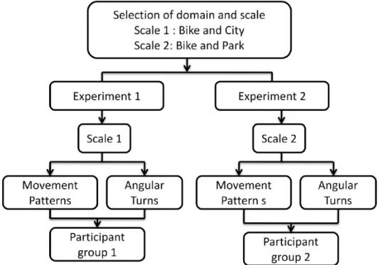
Experiments
Figure 3.1: Experiments Methodology Flowchart
3.2
Experiment 1
In this experiment firstly, we assessed the conceptual knowledge of different move-ment pattern and category construction using a grouping task. Main reason of using the grouping task is that human beings mainly use conceptual knowledge to determine the similarity of given stimuli. Stimuli are placed into the same group if they are considered as similar and they are placed into different groups if they are assumed as dissimilar (Klippel, 2009). Envision of different direction turns is examined in second task of the experiment.
3.2.1
Experiment Material (Task 1)
Figure 3.2: one path of the animated icon
The stimuli size is 120 x 120 pixels. The starting and ending regions are also de-fined as 40 x 70 pixels in size (Klippel and Li, 2009). The starting and ending coordinates are randomized inside the defined boundaries of topologically defined equivalent classes. Ending relation is visually made clear. The speed of the bike is also kept constant in all movement paths. To get the same speed, the path length / frame ratio is normalized i.e. the longer the movement path, the more
frames are used to keep the speed same in all animated stimuli (Klippel and Li, 2009). Between the repetition of the movement path, a small break / pause is kept.
Figure 3.1 shows a path of one animated icon. It is clear that a disconnect re-gion is chosen from which all starting coordinates are selected. Similarly ending coordinates are selected from the defined ending region. Partial overlap is con-sidered as 50 percent overlapping between the bike and the city and between the bike and park as well. The EC, PO and TPP relations coordinates are randomized using only vertical coordinates.
EC-II, DC-II (Fig. 3.2). So we make a distinction of nine possible relations. We decide to select the 3 icons for one topological relation for one equivalent class as we have three paths. So in total we get 27 stimuli for scale one (figure A.3 and figure A.5 in Appendix).
Figure 3.3: Examples of different position of bike passing through the city
3.2.2
Experiment Material (Task 2)
The task two was to analyze the direction concepts which human being thinks and also scrutinize the influence of scale on direction. Different direction/angular cate-gories are assumed in this task. Direction terminology is followed from the Klippel experiment (Klippel and Montello, 2007) as a basis for this research. A full circle (360◦) will be used as a reference for this research. Figure 3.3 demonstrates that
the circle angles start at 6 o’clock and referred to 0◦ and 360◦ degree, 3 o’clock
which is the perpendicular right is called 90◦ , 12 o’clock/straight is referred to as
2007).
Figure 3.4: Depiction of the direction terminology Source:(Klippel and Montello, 2007)
We started with the typical direction model of 45◦, 90◦, 135◦, 180◦, 225◦, 270◦
and 315◦ and sectors are bisected until we got the angular direction differentiating
at the 5.625◦. The back sector angles between 337.5◦ and 22.5◦ were excluded
because of the spiky turns (Klippel and Montello, 2007). All stimuli are constructed using Adobe Flash CS5. Some of stimuli are shown in figure A.5 of Appendix. The shape of the park and city is the same as used in topological segment. Again the stimuli size is 120 x 120 pixels. The speed of the bike is also kept constant in all movement paths. Speed of the animation is also kept constant in all animated stimuli. Between the repetition of the movement path, a small break / pause is kept. 55 stimuli are used for scale one.
3.2.3
Experiment Procedure
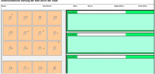
German:Das Fahrrad f¨ahrt durch die dargestellte Stadt und stoppt an verschiede-nen Positioverschiede-nen. Bitte fassen/gruppe sie die Bilder zusammen in deverschiede-nen sie meiverschiede-nen, dass das Fahrrad an der selben Endposition stoppt). In instructions they were told ”Please consider that bike is passing through the city in these images. Bike Stops at different positions. Please make groups of the images in which you think bike stops in similar end positions”. After reading the instructions, a button ’proceed to test’ was placed to precede the experiment.
Figure 3.5: Instructions given for the experiment
Figure 3.6: Screenshot of the window which participant saw initially in experiment 1
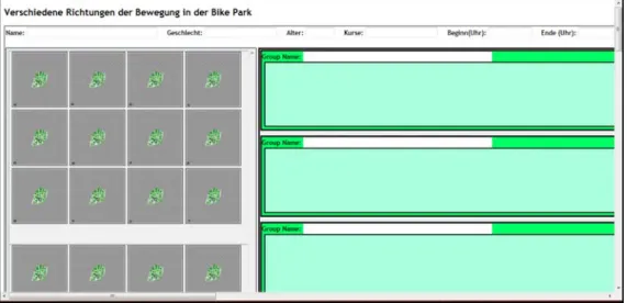
Similarly in task two instructions were also given (In German: Die Bilder zeigen unterschiedliche Richtungen, in die das Fahrrad sich in der Stadt bewegen kann. Bitte gruppiere die Bilder entsprechend ihrer ¨Ahnlichkeit in Bezug auf die Rich-tung des Fahrrads. Erstelle dabei so viele Gruppen wie du m¨ochtest). In this task participants were asked to consider that bike is moving in different directions in the city and to place the stimuli depicting the similar turns of bike in one group and dissimilar into the other groups. Participants were free to choose groups as many as they want. After finishing the task, results were stored by clicking the save option.
3.3
Experiment 2
3.3.1
Experiment Materials (Task One)
We slightly modified the color of the stimuli material from experiment 1. We used 27 animated stimuli and all stimuli were constructed (figure A.6, figure A.7 and figure A.8 in Appendix) using the same methods as in experiment 1. Exactly the same grouping tools were used as in experiment 1 with the same interface.
Figure 3.7: Example of different position of bike passing through the park
3.3.2
Experiment Materials Task two
3.3.3
Experiment Procedure
The procedure for experiment 2 was the same as for experiment 1 except the par-ticipant group. Here again all animated icons were displayed to parpar-ticipants via web page. Again grouping task is used. For task one instructions are provided (In german ’Das Fahrrad f¨ahrt durch die dargestellte park und stoppt an verschiedenen Positionen. Bitte fassen/gruppe sie die Bilder zusammen in denen sie meinen, dass das Fahrrad an der selben Endposition stoppt. In English : Please consider that bike is passing through the city in these images. Bike Stops at different positions. Please make groups of the images in which you think bike stops in similar end positions).By clicking a button proceed to the test” a page was opened. In this page the screen was divided into two parts. All the stimuli material consisting of depicting topological relation is placed on the left side randomly. At the start the right side of the screen was empty. Participants can create the groups of animated icons simply by dragging and dropping. Participants were free to choose groups as many as they can. They could place as many images they want in on group which they considered are similar. After that they were also told to describe the groups in words which they created. (Bitte versuche die verschiedenen Bilder (Fahrradposi-tionen), die du in einer Gruppe zusammengefasst hast, (in Worten) zu beschreiben. Bitte halte die Beschreibung so kurz wie m¨oglich).
so kurz wie m¨oglich).
Chapter 4
Results and Discussion
Cluster analysis allows us to examine the similarities of observations or objects. This method allows one to explore the structure of the data set. In other words, cluster analysis sorts the data into similar clusters that share similar characteristics. The cluster analysis displays the results a tree diagram called dendrogram. The branching-type nature of the dendrogram represents a hierarchy of categories based on degree of similarity.
4.1
Results of Experiment 1
4.1.1
Participants
4.1.2
Task one
The result of the each participant was encoded in a 27 x 27 similarity matrix (table 4.1). The matrix rows and columns correspond to the number of stimuli used in the experiment. It is a symmetric similarity matrix and encodes all possible similarity ratings between two stimuli and produced a matrix of 729 cells. The major purpose of constructing the similarity matrix is that it encodes the results of category by each participant.Once the similarity matrix is obtained, several analyses can be performed to analyze the categorical grouping data, we subjected the similarity matrix to a hierarchical cluster analysis. The analysis was performed using the statistical tool box function of Matlab R2010b with the default similarity measure of Euclidean distance. This is probably the most commonly chosen type of distance. The main advantage of the Euclidean distance is that it considers all possible pairing (Russel A, R., 1999) and is easy to interpret. Mathematically, distance between a pointx (x1, x2 etc.) and a pointy (y1,y2 etc.) is:
d = n i=1
(xi−yi)2 (4.1)
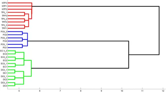
Average, ward’s and complete linkage methods are applied to cross validate the results. All methods show a similar clustering structure. Figure 4.1 and 4.2 shows the resultant dendrograms generated using average and ward method respectively. The variables are represented vertically. The links between the variables are U-Shaped lines. The distances are shown horizontally. The following dendrogram shows the following clusters; NTPP is also forming a distinct cluster and are con-ceptually more similar to the cluster formed by TPP and TPP-II and Showing more similarity among these variables. DC and DC-II relations are assumed to be same and same are the case with the EC and EC-II. DC and EC are also found to be more similar than other relations.
dendro-Figure 4.1: Cluster Analysis using Average linkage method for task 1of Experiment 1
DC1 DC2 DC3 EC1 EC2 EC3 PO1 PO2 PO3 TP P1 TP P2 TP P3 NTP P1 NTP P2 NTP P3 TP PII 1 TP PII 2 TP PII 3 PO II 1 PO II 2 PO II 3 EC II 1 EC II 2 EC II 3 DC II 1 DC II 2 DC II 3 DC1 20 20 12 12 12 0 0 0 0 0 0 0 0 0 0 0 0 0 0 0 10 10 10 12 12 12 DC2 20 20 12 12 12 0 0 0 0 0 0 0 0 0 0 0 0 0 0 0 10 10 10 12 12 12 DC3 20 20 12 12 12 0 0 0 0 0 0 0 0 0 0 0 0 0 0 0 10 10 10 12 12 12 EC1 12 12 12 20 20 5 5 5 1 1 1 0 0 0 0 0 0 4 4 4 14 14 14 9 9 9 EC2 12 12 12 20 20 5 5 5 1 1 1 0 0 0 0 0 0 4 4 4 14 14 14 9 9 9 EC3 12 12 12 20 20 5 5 5 1 1 1 0 0 0 0 0 0 4 4 4 14 14 14 9 9 9 PO1 0 0 0 5 5 5 20 20 3 3 3 0 0 0 0 0 0 16 16 16 4 4 4 0 0 0 PO2 0 0 0 5 5 5 20 20 3 3 3 0 0 0 0 0 0 16 16 16 4 4 4 0 0 0 PO3 0 0 0 5 5 5 20 20 3 3 3 0 0 0 0 0 0 16 16 16 4 4 4 0 0 0 TPP1 0 0 0 1 1 1 3 3 3 20 20 10 10 10 17 17 17 0 0 0 0 0 0 0 0 0 TPP2 0 0 0 1 1 1 3 3 3 20 20 10 10 10 17 17 17 0 0 0 0 0 0 0 0 0 TPP3 0 0 0 1 1 1 3 3 3 20 20 10 10 10 17 17 17 0 0 0 0 0 0 0 0 0 NTP
P1
0 0 0 0 0 0 0 0 0 10 10 10 20 20 10 10 10 0 0 0 0 0 0 0 0 0 NTP
P2
0 0 0 0 0 0 0 0 0 10 10 10 20 20 10 10 10 0 0 0 0 0 0 0 0 0 NTP
P3
0 0 0 0 0 0 0 0 0 10 10 10 20 20 10 10 10 0 0 0 0 0 0 0 0 0 TPP
II 1
0 0 0 0 0 0 0 0 0 17 17 17 10 10 10 20 20 4 4 4 1 1 1 0 0 0 TPP
II 2
0 0 0 0 0 0 0 0 0 17 17 17 10 10 10 20 20 4 4 4 1 1 1 0 0 0 TPP
II 3
0 0 0 0 0 0 0 0 0 17 17 17 10 10 10 20 20 4 4 4 1 1 1 0 0 0 POII 1 0 0 0 4 4 4 16 16 16 0 0 0 0 0 0 4 4 4 20 20 6 6 6 0 0 0 POII 2 0 0 0 4 4 4 16 16 16 0 0 0 0 0 0 4 4 4 20 20 6 6 6 0 0 0 POII 3 0 0 0 4 4 4 16 16 16 0 0 0 0 0 0 4 4 4 20 20 6 6 6 0 0 0 ECII 1 10 10 10 14 14 14 4 4 4 0 0 0 0 0 0 1 1 1 6 6 6 20 20 11 11 11 EC
II 2
10 10 10 14 14 14 4 4 4 0 0 0 0 0 0 1 1 1 6 6 6 20 20 11 11 11 EC
II 3
10 10 10 14 14 14 4 4 4 0 0 0 0 0 0 1 1 1 6 6 6 20 20 11 11 11 DCII 1 12 12 12 9 9 9 0 0 0 0 0 0 0 0 0 0 0 0 0 0 0 11 11 11 20 20 DC
II 2
12 12 12 9 9 9 0 0 0 0 0 0 0 0 0 0 0 0 0 0 0 11 11 11 20 20 DC
II 3
12 12 12 9 9 9 0 0 0 0 0 0 0 0 0 0 0 0 0 0 0 11 11 11 20 20
Table 4.1: Similarity matrix of movement patterns (Exp.1, scale 1)
gram. The cophenetic correlation is a measure of how truly a dendrogram pre-serves the pair wise distances between the original data points. It is defined as ’the linear correlation coefficient between the cophenetic distances obtained from the tree, and the original distances (or dissimilarities) used to construct the tree’ (Mathswork). Cophenetic correlation is the correlation between the actual dis-similarities as recorded in the original dissimilarity matrix, and the disdis-similarities which can be read off of the dendrogram.
Mathematically, the cophenetic correlation is
ρ=
i<j
(dij −d)(d∗ij −d∗)
i<j
(dij −d)2
i<j
(d∗
ij −d∗)2
1/2 (4.2)
Here dij is the euclidean distance between units i and j. d∗ij is the corresponding
minimal distance or cophenetic distance between units i and j in the output den-drogram resulting from some particular hierarchical algorithm. d∗ is the average
distance from a sample size n and defined as following
d= i<j dij
[2 (n2 −n)] (4.3)
The magnitude of the cophenetic correlation coefficient valueρshould be very close to 1 for a high-quality solution (Mouchet et al. 2008). We have calculated the ρ
value against ward, and average method and it gives 0.9790 and 0.9812 respectively.
cluster formed by TPP and TPP-II variables. The result also indicate that the PO and PO-II are found to be in one cluster and are quite far from other clus-ters. Results of linguistic labeling task that participants created are not analysed
Figure 4.3: Euclidean distance model
in much detail. Number of groups varied from 3 to 7. Table 4.2 shows an example for a participant who created four individual groups.
It is identified that linguistic description for each relation varies. Different verbal labeling is found for DC and EC and some of them are; eingeben nicht (does not enter), h¨alt am Anfang der Stadt (stop in the start of the city), h¨alt ausserhalb der Stadt (stop outside the city), Richtung zur Stadt (towards the city), Das Fahrrad beginnt ausserhalb der Stadt und h¨alt ausserhalb der Stadt(the bike start outside the city and stops outside the city) .Some labeling of all NTPP relationsi.e. h¨alt im
No. of Groups
Linguistic Description Stimuli placed in group 1 Das Fahrrad befindet sich
im der Stadt
TPP-1, TPP -2, TPP -3, TPP II-1, TPP II-2, TPP II-3
2 Das Fahrrad h¨alt ausser-halb der Stadt
EC-1, EC-2, EC-3, DC-1, DC-2, DC-3 DCII-1, DCII-2, DCII-3, ECII-1, ECII-2, ECII-3
3 Das Fahrrad h¨alt im Stadtzentrum
NTPP-1, NTPP -2, NTPP -3 4 Das Fahrrad h¨alt an der
Grenze
POII-1, POII-2, POII-3 PO-1, PO-2, PO3
Table 4.2: Linguistic Description created by one participant in Experiment 1 majority of the cases.
4.1.3
Task Two
vectorxs and xt are defined as follows:
Mathematically,
d2
st= (xs−xt)V−1(xs−xt)′ (4.4)
whereV is the n-by-n diagonal matrix whosejth diagonal element is S(j)2, where
S is the vector of standard deviations.
Average, wards’s, single and complete linkage methods are applied to cross val-idate the results. Outcome of ward’s method (Figure 4.6) gives compact clusters, while single method (Figure 4.4) gives a chain type clustering. Dendorgrams pre-pared by all methods shows the seven different categories; Left (L), Right (R), Right Front (RF), Left Front (LF), Right Back (RB) and Left Back (LB). These seven categories are characterized by the participants in experiments. The right and left turn angular boundaries are varying in different groups which mean that no participant grouped perpendicular axis (90◦ and 270◦) alone. It is also
scruti-nized that angles around 73◦ to 106◦are mostly perceived as right turns and angles
around 247◦ to 286◦ as left turns. The straight ahead 180◦ axis is not grouped
alone. The clusters formed by right front (turn from 112◦ to 163◦ ) and left front
(turn from 196◦ to 247◦) also shows the right front and left front parts. The right
and left back turns are also discriminated from the other sectors.
To compare a model of the similarity behavior to actual behavior in the dendor-gram plotted above, we measured cophenetic correlation coefficient for all cluster-ing methods. ρ values (0.970 for average linkage method, 0.9439 for ward method, 0.9707 for single method and 0.9564 for complete method) are very close to one shows that dendrograms plotted from all methods shows a good fit model of simi-larity behavior.
Figure 4.4: Cluster Analysis using Single linkage method for task 2 of Experiment 1
Figure 4.6: Cluster Analysis using Ward’s method for task 2 of Experiment 1 macht einen starken Knick, fast parallel zum Anfangsstartpunkt (straight, then turn left. The road makes a sharp bend, almost parallel to the initial starting point), gerade aus, dann rechts abbiegen. Die Strasse macht einen starken Knick, fast parallel zum Anfangsstartpunkt (straight, then turn right. Road makes a sharp bend, almost parallel to the initial starting point), Rechts nach hinten abbiegen (Towards Right back), Links nach hinten abbiegen (towards Left back ). In some cases, right and left back turns are also labeled as; Das Fahrrad biegt in eine stark gekr¨ummte Rechtskurve ab (bike makes a strong right back turn) and biegt in eine stark gekr¨ummte Linkskurve ab( bike makes a strong left back turn).
4.2
Results of Experiment 2
4.2.1
Participants
20 participants (11 females and 9 male) of homogeneous language (German only) from the University of Mnster, Department of physics and Mathematics and Uni-versity of Duisburg Essen are participated in the experiment. All participants were the university students having different study backgrounds (Chemistry, Physics, Mathematics, Biology and Engineering) including two participants who had the cognitive science back ground. Participant’s age was between the 22 to 36 years. The participants took 20-35 minutes for first task and 20 to 50 minutes for the second task. Participants were not paid for the experiment and they performed the experiment on voluntary basis.
4.2.2
Task one
The grouping of each participant results in a 27 x 27 similarity matrix (table 4.3). It is a symmetric similarity and has 729 cells.Likewise the experiment 1, we performed the hierarchical cluster analysis with the default similarity measure of Euclidean distance to analyze the categorical grouping data. Three different clustering meth-ods: Ward, average linkage and complete are used to generate dendrograms. All methods shows a similar clustering structure (Figure 4.7 and 4.8). From the figure 26 we can examine the grouping behavior of the NTPP which is not grouped alone but mostly grouped with TPP and TPP-II relations. TPP, TPP-II and NTPP are found similar to each other than other relations. DC and EC are also conceived as similar. Linkage pattern in shows that TPP, TPP-II and NTPP are seems to be more similar than other relations. All equivalent classes of DC and DCII are appeared in one cluster and same is the case with EC and ECII relations. Cluster-ing structure of DC and EC shows that these are conceptually similar each other. Figure also shows that clusters formed by PO and POII meet at very high distance with the joint cluster of DC and EC which shows a higher dissimilarity.
0 DC1 DC2 DC3 EC1 EC2 EC3 PO1 PO2 PO3 TP P1 TP P2 TP P3 NTP P1 NTP P2 NTP P3 TP PII 1 TP PII 2 TP PII 3 PO II 1 PO II 2 PO II 3 EC II 1 EC II 2 EC II 3 DC II 1 DC II 2 DC II 3 DC1 20 20 10 10 10 0 0 0 0 0 0 0 0 0 0 0 0 0 0 0 8 8 8 15 15 15 DC2 20 20 10 10 10 0 0 0 0 0 0 0 0 0 0 0 0 0 0 0 8 8 8 15 15 15 DC3 20 20 10 10 10 0 0 0 0 0 0 0 0 0 0 0 0 0 0 0 8 8 8 15 15 15 EC1 10 10 10 20 20 1 1 1 0 0 0 0 0 0 0 0 0 1 1 1 17 17 17 7 7 7 EC2 10 10 10 20 20 1 1 1 0 0 0 0 0 0 0 0 0 1 1 1 17 17 17 7 7 7 EC3 10 10 10 20 20 1 1 1 0 0 0 0 0 0 0 0 0 1 1 1 17 17 17 7 7 7 PO1 0 0 0 1 1 1 20 20 2 2 2 0 0 0 1 1 1 19 19 19 1 1 1 0 0 0 PO2 0 0 0 1 1 1 20 20 2 2 2 0 0 0 1 1 1 19 19 19 1 1 1 0 0 0 PO3 0 0 0 1 1 1 20 20 2 2 2 0 0 0 1 1 1 19 19 19 1 1 1 0 0 0 TPP1 0 0 0 0 0 0 2 2 2 20 20 16 16 16 18 18 18 0 0 0 0 0 0 0 0 0 TPP2 0 0 0 0 0 0 2 2 2 20 20 16 16 16 18 18 18 0 0 0 0 0 0 0 0 0 TPP3 0 0 0 0 0 0 2 2 2 20 20 16 16 16 18 18 18 0 0 0 0 0 0 0 0 0 NTP
P1
0 0 0 0 0 0 0 0 0 16 16 16 20 20 14 14 14 0 0 0 0 0 0 0 0 0 NTP
P2
0 0 0 0 0 0 0 0 0 16 16 16 20 20 14 14 14 0 0 0 0 0 0 0 0 0 NTP
P3
0 0 0 0 0 0 0 0 0 16 16 16 20 20 14 14 14 0 0 0 0 0 0 0 0 0 TP
II 1
0 0 0 0 0 0 1 1 1 18 18 18 14 14 14 20 20 2 2 2 1 1 1 0 0 0 TP
II 2
0 0 0 0 0 0 1 1 1 18 18 18 14 14 14 20 20 2 2 2 1 1 1 0 0 0 TP
II 3
0 0 0 0 0 0 1 1 1 18 18 18 14 14 14 20 20 2 2 2 1 1 1 0 0 0 POII 1 0 0 0 1 1 1 19 19 19 0 0 0 0 0 0 2 2 2 20 20 2 2 2 0 0 0 POII 2 0 0 0 1 1 1 19 19 19 0 0 0 0 0 0 2 2 2 20 20 2 2 2 0 0 0 POII 3 0 0 0 1 1 1 19 19 19 0 0 0 0 0 0 2 2 2 20 20 2 2 2 0 0 0 ECII 1 8 8 8 17 17 17 1 1 1 0 0 0 0 0 0 1 1 1 2 2 2 20 20 8 8 8 EC
II 2
8 8 8 17 17 17 1 1 1 0 0 0 0 0 0 1 1 1 2 2 2 20 20 8 8 8 EC
II 3
8 8 8 17 17 17 1 1 1 0 0 0 0 0 0 1 1 1 2 2 2 20 20 8 8 8 DCII 1 15 15 15 7 7 7 0 0 0 0 0 0 0 0 0 0 0 0 0 0 0 8 8 8 20 20 DC
II 1
15 15 15 7 7 7 0 0 0 0 0 0 0 0 0 0 0 0 0 0 0 8 8 8 20 20 DC
II 3
15 15 15 7 7 7 0 0 0 0 0 0 0 0 0 0 0 0 0 0 0 8 8 8 20 20
Table 4.3: Similarity matrix of movement patterns (Exp.2, scale 2)
Figure 4.7: Cluster Analysis using ward’s method for task 1 of Experiment 2
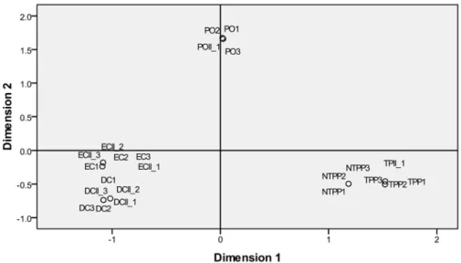
ward’s method) and 0.9952 (for average linkage method) validate the faithfulness of dendrogram. Similarly, MDS technique is applied to validate the results. The resultant perceptual map depicts the relative positioning of all variables. From figure 4.9 it is clear that three clear clusters. TPP, TPP-II and NTPP variables are appeared to be in one cluster and far from the cluster formed by DC and EC variables. Both PO and PO-II are placed far away forming one cluster.
Figure 4.9: Euclidean distance model for scale 2
No. of Groups
Linguistic Description Stimuli placed in group 1 Das Fahrrad ber¨uhrt die
Grenzen des Parks.
POII-1, POII-2, POII-3 PO-1, PO-2, PO3 2 Das Fahrrad befindet sich
in der N¨ahe des Parks.
EC-1, EC-2, EC-3, 1, 2, ECII-3,
3 Das Fahrrad hat den Park befahren
TPP-1, TPP-2, TPP-3, 1, TPPII-2, TPPII-3, NTPP-1, NTPP-TPPII-2, NTPP-3, 4 Das Fahrrad befindet sich
weit vom Park entfernt
DC-1, DC-2, DC-3 1, 2, DCII-3
Table 4.4: Linguistic Description created by one participant in Experiment 2
4.2.3
Task two
We prepared a similarity matrix 55 x 55 (table A.2 in Appendix). Likewise the experiment 1, hierarchical cluster analysis is performed using the similarity mea-sure standardized Euclidean distance. Reason of using the standardized Euclidean distance is the numerical scale of the variables found in similarity table. Aver-age, wards’s, single and complete linkage methods are applied to cross validate the results. Clustering structure does not find to be different as compared to the results of experiment 1. In all dendorgrams seven different categories are found as in experiment one. Figures 4.10, 4.11 and 4.12 shows the results of single link-age, ward’s and average method. Dendrogram prepared by ward’s method gives compact clustering structure.
To compare a model of the similarity behavior to actual behavior in the dendor-gram plotted above, we measured cophenetic correlation coefficient for all clustering methods. ρvalues (0.970 for average linkage method, 0.9439 for ward method and 0.9565 for Single linkage) are very close to one shows that dendrograms plotted from all methods shows a good fit model of similarity behavior.
par-Figure 4.10: Dendrogram generated using Single linkage method (Task 2 of Exper-iment 2)
Figure 4.12: Dendrogram generated using Average linkage method (Task 2 of Ex-periment 2)
ticipants. As an example, for a participant who created seven individual groups; nach links (left ), nack rechts (right), immer gerade aus (straight), nach richts oben (right front), nach links oben (left front), rechts nach hinten abbiegen (Right back), links nach hinten abbiegen (Left back). We also find the description of Right front and left front sectors as biegt leicht nach links ab (turn slightly left), biegt leicht nach rechts ab (turn slightly right). Another seven individual groups created by a participant also described in the following way; nach Osten (East), nach Westen (West), nach Norden (North), nach S¨udosten (Southeast), S¨udwesten (Southwest), Nordosten (Northeast), Nordwest (northwest).
4.3
General Discussion
different scale i.e. bike and park where mostly NTPP is grouped with the TPP
and TPP-II relations instead of grouped separately. The experiment results are the same as Klippel (2009) that TPP, TPP-II and NTPP are conceptually very close but it is also find that NTPP is mostly categorized single in scale 1, where as in scale 2 i.e. bike and park NTPP grouping is found to more with TPP and
TPP-II relations. it can be assumed that participants are considering the NTPP relation specifically as city centre in case of scale one which can be shown by their linguistic description they created. While in case of scale 2, mostly it is not treated as specifically.
In both experiments, we find that DC, EC are found close as they are grouped together. Another finding of the study is that DCII and ECII relations are also found in one group but separate from the group formed by DC and EC relations. This shows that DC and EC are treated as the starting point of the path followed by bike and DCII and ECII are assumed as end of the bike path. It is also examine that DC and EC grouping does not make a difference in our selected domain of scale. One reason could be the design and construction of the stimuli and partici-pants assumed that bike path is started only from starting region. It would be an interesting question what would be the results if we have different starting region for different paths of bike.
Similarly, fusion coefficient for cluster joining the DC and EC is 6.573. On the contrary the fusion coefficient for clusters DC/EC and PO/PO-II is 12 gives result of higher dissimilarities among these variables.
In the second task of both experiments, the grouping behavior of different direction turns seems not affected by influence of scale. It is found that participants created seven to nine individual groups. The right and left turn angular boundaries are varying in different groups. It is also observed that no participant grouped per-pendicular axis alone and is grouped with more than 4 icons. It is also scrutinized angles around 73◦ to 106◦ are mostly perceived as right turns and angles around
247◦ to 286◦ as left turns. It means that the demarcation of front and back plane
is not found which is similar to the results of ’non linguistic awareness experiment 2, the research conducted by Klippel in 2007. Beside, right and left front parts are identified. Angles around (112◦ -163◦) are assumed as right front turns while
angles around (196◦ to 247◦) are perceived as left front turns. Furthermore, Back
turns and sharp back turns distinction is also recognized which was not expected. It might be because of the technical study background of participants. In sharp direction turns bike is assumed that bike is coming back to its starting position which participants justified in their verbal labeling.
Chapter 5
Conclusion
5.1
Research Findings
and do not make any difference of characterizing in both scales. In conclusion we found four distinct groups in case of scale 1 and three in case of scale two which is because of the grouping of NTPP. The result of the grouping is found to be more similar to the research conducted by Klippel (2009) but found to be different from the study conducted by Lu and Harter, who showed that humans have the procliv-ity toward simplification in constructing different temporal relations. Directional relations conceptualization is also a most important aspect of spatial reasoning. We examined influence of scale on the categorization of the direction turns when they are grouped into similarity basis but do not find the diverse results. It is clearly seen from the results that direction turns right, left, front, back and even sharp turns are distinguished and indicate the awareness about the different direction categories in human mind. This research does not find difference in categorization of different direction turn when experienced on two different scales i.e. bike and
city and bike and park, one factor could be the design of the material and another might be strong technical background of the participants.
5.2
Future Work
Bibliography
[1] Allen, J. F., (1983), Maintaining knowledge about temporal intervals, Com-munications of the ACM, 26, pp-832-843.
[2] Aldenderfer, M. S., & Blashfield, R. K., (1984), Cluster Analysis, Sage university paper series on quantitative applications in the social sciences, Newbury Park, CA: Sage, pp-07-044.
[3] Casati, R., (2000), Topology and cognition, Encyclopedia of cognitive sci-ence, McMillan Nature Publishing Group, vol. 4, pp-410-417.
[4] Cohn, A.G., Bennett, B., Gooday, J., and Mark, N.G., (1997), Quali-tative Spatial Representation and Reasoning with the Region Connection Calculus In Proceedings of the DIMACS International Workshop on Graph Drawing, Lecture Notes in Computer Science, Journal Geoinformatics, Vol-ume 1, Number 3, pp- 275-316.
[5] Chang, S.K., Shi, Q.Y., & Yan, C., (1987), Iconic indexing by 2D strings, IEEE Transactions on Patter Analysis and Machine Intelligence, 9 (3), pp-413-428.
[7] Egenhofer, M.J., (1997), Query processing in Spatial-Query-by-Sketch, Journal of Visual Languages and Computing, 8 (4), pp- 403-424.
[8] Egenhofer, M.J., Mark, D. and Herring, J., (1994), The 9 Intersection, formalization and its use for natural language spatial predicates, NCGIA Technical Report, pp-94-1.
[9] Egenhofer, M. J., & Al-Taha, K. K., (1992), Reasoning about gradual changes of topological relationships, In A. U. Frank, I. Campari, & U. Formentini (Eds.), Theories and Methods of Spatio-temporal Reasoning in Geographic Space, pp- 196-219.
[10] Egenhofer, M. J., & Franzosa, R. D., (1991), Point-set topological spatial relations, International Journal of Geographical Information Systems, 5(2), pp- 61-174.
[11] Frank, A.U., (1996), Qualitative spatial reasoning: cardinal directions as an example, International journal of Geographical information system, 10, 3, pp-269-290.
[12] Frank, A.U., (1990), Qualitative spatial reasoning about cardinal direc-tions, In Autocarto 10, Edited by D.M Mark and D.White, Baltimore: ACSM/ASPRS.
[13] Frank, A.U., Campari, I. (eds.): Spatial Information Theory: Theoretical Basis for GIS. Lecture Notes in Computer Science, Vol. 716. Springer Ver-lag. pp-312-321 In Montello, D. (1993), Scale and multiple psychologies of space, In A.U.Frank & I.Campari (Eds.), spatial information theory: A theoretical basis for GIS, pp. 312-321.
[15] Freksa, C., (1992), Temporal reasoning based on semi-intervals. Artificial Intelligence, 54(1), 199-227.
[16] Freeman, J., (1975), The modeling of spatial relations, Computer Graphics and Image processing 4, pp-156-171.
[17] Goyal, R., (2000), Similarity assessment for cardinal directions between extended spatial objects, Ph.D. Dissertation, Department of Surveying En-gineering, University of Maine.
[18] Grling, T., and Golledge, R.G., (1987), Environmental perception and cog-nition, E.H. Zube, G.T. Moore (eds.), Advances in environment, behavior, and design, Vol. 2, pp- 203-236, In Montello, D. (1993), Scale and multiple psychologies of space, In A.U.Frank & I.Campari (Eds.), spatial informa-tion theory: A theoretical basis for GIS, pp. 312-321.
[19] Haar, R., (1976), Computational models of spatial relations, Technical Report, University of Maryland, College Park, Department of Computer Science.
[20] Hill, L. (2006), Geo referencing, the geographic associations of information, , chapter 2, spatial cognition and information system, Massachussetes in-stitute of technology, pp- 23
[21] Hubona G.S., Everett, S., Marsh, E., and Wauchope,K., (1998), Mental representation of spatial language, Int. Journel of human computer Studies, Volume 48, pp.705-728.
[22] Holgersson, M., (1978), The Limited value of Cophenetic Correlation as a clustering criterion margareta, Volume 10, pp- 287-295.
[24] Jing, W., Gang, J., and Rui, G. (2008), Qualitative detailed description for spatial direction Relations , Zhengzhou Institute of Surveying and Map-ping, China.
[25] Klippel, A., Dewey, C., Knauff, M., et al., (2004), Direction concepts in way finding assistance systems, Workshop on Artificial Intelligence in Mobile Systems, pp- 1-8.
[26] Klippel, A. (2009), Topologically Characterized Movement Patterns, A Cognitive Assessment’, Spatial Cognition & Computation, 9: 4, pp- 233 -261.
[27] Klippel, A., and Montello, D.R., (2007), Linguistic and nonlinguistic turn direction concepts, S Winter at al.(Eds), LNCS 4736, pp-354-372.
[28] Klippel, A., and Li, R., (2009), The Endpoint Hypothesis, A Topological-Cognitive Assessment of Geographic Scale Movement Patterns, Volume 5756, pp-177-194.
[29] Kurata, Y., (2008), The 9-Intersection: A Universal Framework for Mod-eling Topological Relations, In Proceedings of GIScience, T.J. Cova et al. Eds, PP- 181-198.
[30] Kuarata, Y., and Egenhofer, M.J., (2007), The 9+Intersection for Topo-logical Relations betweena Directed Line Segment and a Region, Gottfried, B. (ed.) 1st International Symposium for Behavioral Monitoring and In-terpretation, Universitaet Bremen TZI Technical Report 42, pp-62-76. [31] Kuipers, B., (1978), Modeling spatial knowledge, Cognitive Science 2,
pp-129-153 In Mark, M., and Frank, A.U., (1989), concepts of space and spa-tial language, Proceedings, Ninth International Symposium on Computer-Assisted Cartography (Auto-Carto 9), Baltimore, Maryland, pp- 538-556. [32] Krishnapuram,A., Keller, J.M., and Ma, Y., (1993), Quantitative analysis
[33] Kruskal, J.B. and Wish, M. (1978), Multidimensional Scaling. Beverly Hills, CA: Sage Publications.
[34] Loomis, J. M., Da Silva, J. A., Philbeck, J. W. & Fukusima, S. S. (1996), Visual perception of location and distance, Current Directions in Psycho-logical Science, 3, pp-72-77.
[35] Li, S., and Liu, w., (2010), Topological Relations between Convex Regions, in Proceedings of the 24th AAAI Conference on Artificial Intelligence, At-lanta, Georgia, USA.
[36] Lu, S., Harter, D., (2006), The role of overlap and end state in perceiving and remembering events. In: Sun, R. (ed.), The 28th Annual Conference of the Cognitive Science Society, Vancouver, British Columbia, Canada, pp-1729-1734.
[37] Mark, M., and Frank, A.U., (1989), concepts of space and spatial language, Proceedings, Ninth International Symposium on Computer-Assisted Car-tography (Auto-Carto 9), Baltimore, Maryland, pp- 538-556.
[38] Marks, D., and Egenhofer, M., (1994), Modeling spatial relations between lines and regions: Combining formal mathematical models and human sub-jects training, Cartography Geographic Inform, Systems 21(4), pp- 195-212.
[39] Montello, D. (1993) Scale and multiple psychologies of space, In A.U.Frank & I.Campari (Eds.), spatial information theory: A theoretical basis for GIS, pp- 312-321.
[41] Miyajima, K., and Ralescu, A., (1994), Spatial organization in 2D seg-mented images: Representation and recognition of primitive spatial rela-tions, Fuzzy Sets and Systems, pp- 225-236.
[42] Miyajima, K., and Ralescu, A., (1994), Spatial organization in 2D images, Proc. 3rd IEEE Internat. Conf. on Fuzzy Systems, FUZZ-IEEE, pp- 100 105.
[43] Mouchet, M., Guilhaumon, F., Villeger, S., Mason, N. W. H., Tomasini, J. A. and Mouillot, D., ( 2008), Towards a consensus for calculating dendrogram-based functional diversity indices. Oikos 117, pp-794-800. [44] Mathworks, statistical tool box.
[45] Peuquet, D.J., and CI-Xiang, Z., (1987), An algorithm to determine the directional relationship between arbitrarily-shaped polygons in the plane, Pattern Recognition, 20 (1), pp-65-74.
[46] Petchey, O.L., Evans, K.L., Fishburn, I.S., and Gaston, K.J., ( 2007) Low functional diversity and no redundancy in British avian assemblages. J. Anim. Ecol. 76: pp-977-985.
[47] Petchey, O. L. and Gaston, K. J., (2006), Functional diversity: back to basics and looking forward. Ecol. Lett. 9: pp-741-758.
[48] Randell, D.A., Cui, Z., and Cohn, A.G., (1992), A Spatial Logic based on Regions and Connection, 3rd international conference on knowledhe representation and reasoning, Morgan Kaufmann, pp-165-176.
[49] Romesburg, H.C., (1984), Cluster analysis for researcher, chapter seven: standardization the data matrix, Belmont, Calif Lifetime Learning Publi-cations, pp-75-92.
[51] Schober, M. (1993) Spatial perspective taking in conversation, Cognition, Volume 47, pp-1-24.
[52] Schwering, A., (2007), Evaluation of a semantic similarity measure for nat-ural language spatial relations.In: Winter, S., Duckham, M., Kulik, L., Kuipers, B. (eds.) LNCS, vol. 4736, Springer, Heidelberg, pp-116-132 . [53] Talmy, L (1978), How language structure space , In Vorwerg, C., &
Rick-heit, G., (1998), Typical effects in categorization of spatial relations in Spatial Cognition, An Interdisciplinary Approach to Representing and Pro-cessing Spatial Knowledge, LNCS (LNAI), Vol. 1404, pp-203-222.
[54] Taylor, T.E., Gagne, C.L., and Eagleson, R., (2000), Cognitive Constraints in Spatial Reasoning: Reference Frame and Reference Object Selection. American association for artificial intelligence technical report SS -00-04 pp. 168-172.
[55] Vorwerg, C., & Rickheit, G., (1998), Typical effects in categorization of spatial relations in Spatial Cognition, An Interdisciplinary Approach to Representing and Processing Spatial Knowledge, LNCS (LNAI), Vol. 1404, pp-203-222.
[56] Wang, X., and Keller, J.M., (1999), Human-based spatial relationship gen-eralization through neural/fuzzy approaches, Fuzzy Sets and Systems 101, pp- 5-20.
[57] Yang, K., and Trewn, J., (2004), Multivariate statistical methods in quality management, chapter seven: cluster analysis, McGraw-Hill, pp-181-200. [58] Zahn, C. T., (1971), Graph-theoretical methods for detecting and
Appendix A
Appendix 1
Figure A.1: Second path of bike (animated icon) passing through the city
Figure A.3: 9 Different position of bike (path 1)
Figure A.5: Different direction paths of bike (Exp. 1, scale 1)
Figure A.7: Path 2 (bike passing through the park)