The portuguese households? Indebtedness

M

ESTRADO

M

ONETARY AND

F

INANCIAL

E

CONOMICS

T

RABALHO

F

INAL DE

M

ESTRADO

D

ISSERTAÇÃO

T

HE

P

ORTUGUESE

H

OUSEHOLDS

’

I

NDEBTEDNESS

M

ESTRADO

M

ONETARY AND

F

INANCIAL

E

CONOMICS

T

RABALHO

F

INAL DE

M

ESTRADO

D

ISSERTAÇÃO

T

HE

P

ORTUGUESE

H

OUSEHOLDS

’

I

NDEBTEDNESS

R

ITA

M

ARIA

H

ENRIQUES

P

EREIRA

S

:

Rita Maria Henriques Pereira

Supervisor: João Ferreira do Amaral

Master in Monetary and Financial Economics

ABSTRACT 

Since the 2008’s financial crisis authorities have been particularly aware about the necessity of being provided with “early warning indicators” regarding financial stability. In fact, the Basel Committee on Banking Supervision suggests the analysis of the difference between the private sector credit-to-GDP ratio and its own long-term trend even though it has been criticized for its poor suitability to countries that have had a rapid credit build-up. For the past two decades Portugal has witnessed a dramatic indebtedness increase among households and the aim of this paper is precisely to examine the reasons for this increase by analysing the ratio of domestic credit to the private sector to GDP. The main conclusions are the non-suitability of the Basel Committee on Banking Supervision approach for Portugal and the break of the link between deposits and credit from 1992 onwards.

ACKNOWLEDGMENTS 

Firstly I would like to thank my supervisor Professor João Ferreira do Amaral for being available and interested in guiding this thesis and for suggesting the topic. Professor had an unimaginable patience with my doubts and insecurities and it has been my pleasure and honour to work with Professor João. I also would like to thank Professor António Afonso for always being available in helping me with the empirical analysis.

Secondly, I would like to thank my dearest and best friends Ana, Carina, Margarida, Maria João, Pedro and Sandra for their friendship and kindness and for always believing in me. To my boyfriend Vasco for his support during occasional meltdowns and for always reminding me how far I have come. Plus, I would like to thank José not only for suggesting a paper that saved this thesis but also for his friendship and Raquel for her incredible support throughout these two intensive and stressful years.

Finally, I would like to thank my foundation and my everything, which is my family. This paper is dedicated to my father Jorge, my mother Paula, my grandmother Totas and my sister Inês. Thank you for your endless support during this seven-year adventure with two degree changes, many ugly cries and happiness. Thank you for always lifting me up when I thought I had enough. Thank you for always trusting in me and supporting my decisions even when everyone thought I was absolutely crazy. Thank you for your unconditional love.

CONTENTS 

1 |

INTRODUCTION...5

2 |

LITERATURE REVIEW ...6

3 |

PORTUGUESE HOUSEHOLDS’ INDEBTEDNESS...8

4 |

THE RATIO AS AN INDICATOR ...14

5 |

EMPIRICAL ANALYSIS ...17

6 |

CONCLUSIONS...31

7 |

REFERENCES ...33

APPENDIX 

LIST OF FIGURES AND TABLES

FIGURE 1 ‐ Domestic Credit to Private Sector for Portugal as % of GDP (1961‐2011)... 9 

FIGURE  2  –Long‐term  Interest  Rate  for  Convergence  Purposes  for  Portugal  (1993‐ 2012)... 12 

FIGURE  3  ‐  Annual  Portuguese  GDP  and  DCPS  Growth  Rates  (1961‐ 2011)... 18  FIGURE 4 ‐ FIGURE 4 ‐ State Probabilities of the DCPS‐to‐GDP Ratio for Portugal (1961‐ 2011)... 21  FIGURE 5 ‐ Bank Credit to Bank Deposits Ratio (%) for Portugal (1961‐2011)... 28  FIGURE 6 ‐ Select European Countries Levels of Financial Deepening (1999−2010)... 37  FIGURE 7 ‐ Número de Contratos Celebrados... 37  FIGURE 8 – Current Account Balance as % of GDP (1980−2011)... 41 

FIGURE  9  –  Comparison  between  Current  Account  Balance  and  the  Bank  credit‐to‐  Bank deposits Ratio... 41  TABLE I ‐ Constant Markov Transition Probabilities Matrix... 38  TABLE II – Granger Causality Tests... 38  TABLE III – Long‐run Estimates of Portuguese GDP... 39  TABLE IV – Long‐run Estimates of Portuguese DCPS... 39  TABLE V – Vector Error Correction (VEC) Model... 40 

1 | INTRODUCTION 

The Portuguese households’ indebtedness has not been receiving the deserved attention. Since the 1990 decade the levels of indebtedness have been increasing dramatically and the main reason is the households’ housing demand that fuelled a rapid credit growth.

The situation should not be ignored. Indebted households are more vulnerable to unanticipated shocks - such as unemployment, a decrease in disposable income or an interest rate increase- which increases the probability of default and, consequently, threats the country’s financial stability. Therefore having indicators that may help authorities to signal periods of excessive credit (which usually result in financial instability) became a major concern, particularly since the 2008’s financial crisis.

In fact, the Basel Committee on Banking Supervision (BCBS) suggests the use of the Hodrick-Prescott (HP) filter to determine the Private Sector credit-to-GDP gap i.e., the difference between the credit-to-GDP ratio and its own long-term trend, and recommends it as a common starting point for authorities to determine whether there is an excessive credit growth or not. These so-called “early warning indicators” should be seriously considered although judgement is always recommended when authorities make their decisions. The BCBS approach has been criticized because it has not been considered appropriate to countries that had a rapid credit build-up.

The empirical analysis of this paper is based on Kelly et al (2011) and only Portugal’s case will be explored. The main findings are the non-suitability of BCBS approach to Portugal and the break of the deposits-credit link from 1992 onwards.

The paper is organized as follows. There is a brief historical context of the Portuguese economy since the 1950’s and the main reasons that led households to get into debt. Then, the importance of the “early warning indicators” and the criticism to the BCBS approach are explained. Afterwards there is the empirical analysis: a two-state Markov Switching model to analyse structural breaks of the Domestic Credit to Private Sector (DCPS) -to-GDP ratio and OLS and DOLS regressions in order to analyze the long-run relationship between DCPS and GDP in specific periods. Finally the main conclusions are summarized.

2 | LITERATURE REVIEW 

The Portuguese households’ indebtedness is not a heavily studied subject and the main papers about it were produced by the Economic Research Department of Banco de

Portugal.

Farinha & Noorali (2004) use the data from the 2000’s Households’ Wealth and Indebtedness Survey to analyse aggregate indicators regarding Portuguese households’ wealth and indebtedness. The authors show how credit to house purchase is the main reason for households’ indebtedness and although households’ wealth has increased for the then past two decades, households’ indebtedness grew even more. The authors do not consider that the more vulnerable households (indebted young families) represent any risk to financial stability even though they acknowledge that these highly indebted households would be extremely affected if facing unemployment, income reduction or an interest rate increase.

Castro (2006) elaborates a model where consumers may have liquidity constraints in order to study the Portuguese households’ sensitivity of consumption to disposable income. It is shown a reduction in liquidity constraints in the 1990 decade due to the interest rates decrease and the increase of financial liberalization. It increases at the end of the same decade and the beginning of the 2000’s because households’ indebtedness increase as a percentage of the disposable income.

Farinha (2007) uses the data from 2006/2007’s Households’ Wealth and Indebtedness Survey to analyze the Portuguese households’ indebtedness. Again, the author concludes that the most vulnerable households are young and low income families but since their share in the debt market is relatively low comparing to the total, there are small or no risks to financial stability.

Costa & Farinha (2012) make a microeconomic analysis of the results from the 2010’s Households’ Financial and Consumption Survey. It concludes that the upward trend of the households’ indebtedness throughout the last two decades has been interrupted as consequence of the Economic Adjustment Programme that Portugal is under since 2011. From the survey’s results the authors also conclude that the percentage of households who are unable to meet their financial obligations is low but likely to increase due to the country’s difficult macroeconomic environment (such as unemployment and decrease of disposable income). Again, Costa & Farinha (2012) argue that the most vulnerable households are the low income and young households who are indebted. Even though young families’ participation in the debt market is high, the amounts borrowed are not significant when comparing to the total, plus their debts are supported in real estate. Therefore, the authors consider that in case of default, the impact on the financial stability would be mitigated.

Costa (2012) also uses 2010’s Households’ Financial and Consumption Survey to determine the probability of default taking into account the households’ economic and socio-demographic features. As Costa & Farinha (2012), Costa (2012) concluded that low income households are the ones with higher probability of default. It shows that households’ who have defaulted did so due to unexpected shocks in their financial situation, such as unemployment, and it would have not happen if it were for these unanticipated shocks. Therefore, the author explains that this situation shows how households were rational when taking credit decisions i.e., if no shocks had occur the indebted families would have continued to be able to meet their financial commitments.

It is obvious that conclusions tend to be rather repetitive throughout the years and it starts to become little bit clear how the institution had a passive attitude towards the problem for the past two decades– a topic that will be address in section 5.4.

3 | PORTUGUESE HOUSEHOLDS’ INDEBTEDNESS 

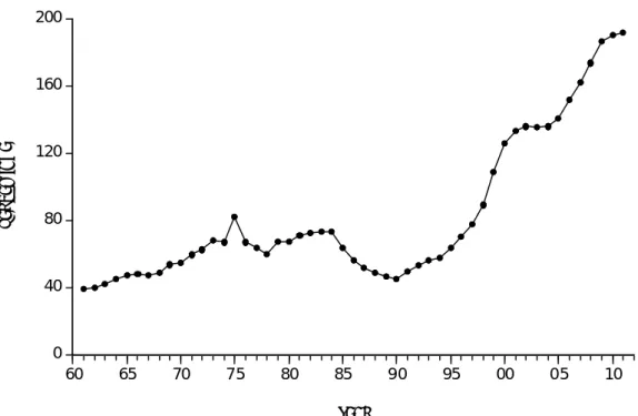
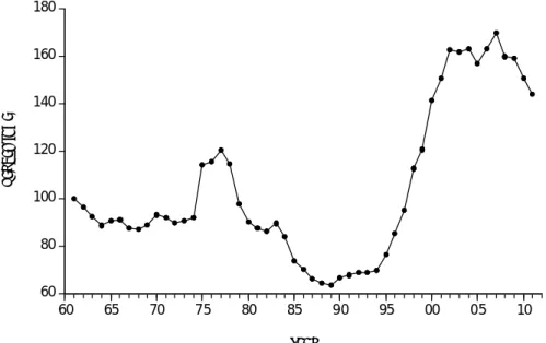
The Portuguese households’ indebtedness is definitely a topic worth looking closely due to its peculiar evolution. Portugal is a small and open economy and its households have worrisome levels of indebtedness. According to Castro (2006), in 1990 the households’ indebtedness was 20 per cent of the disposable income, in 1995 was 40 per cent and by 2004 it was already 118 per cent. And until 2011 it had not slowed down. Figure 1 illustrates this staggering situation:

FIGURE 1 ‐ Domestic Credit to Private Sector for Portugal as % of GDP (1961‐2011)   Source: World Development Indicators.  0 40 80 120 160 60 65 70 75 80 85 90 95 00 05 10 PE R C EN TA G E YEAR

Figure 1 displays the Domestic Credit to Private Sector (DCPS) as a percentage of Growth Domestic Product (GDP). This ratio is a widely used indicator as it will be explained in chapter 4.

It is perfectly clear the increasing trend in households’ indebtedness, particularly from the 1990 decade onwards. And, as Kelly et al (2011) show, Portugal was not alone in this trajectory since some countries have gone through a similar experience, such as Ireland, United Kingdom, Spain and the Netherlands1.

In order to understand the possible reasons for this behaviour it is worth making a mini flashback of the country’s evolution for the past few decades.

After the Second World War, Portugal enjoyed the so-called “golden years” of the world’s economic growth that began in 1950. Plus, Portugal’s integration on several

1

economic organizations - such as Organization for Economic Co-operation and Development (OECD), European Free Trade Association (EFTA), General Agreement on Tariffs and Trade (GATT) and European Economic Community (ECC) -, led to a huge integration of the country’s economy. However in the 1970 decade the situation changed: there were two oil shocks (1973 and 1979), the collapse of the Bretton Woods System and, most importantly, the April 25th Revolution that ended the forty-one-year

dictatorial regime in Portugal.

Although Portugal had been set free from the oppressive regime it was under, the 1970’s were a rough decade. In May 1978 Portugal had no choice but to ask for the International Monetary Fund (IMF) help in order to stabilize the troubling macroeconomic environment felt at the time. When the second oil crisis occurred in 1979, which was obviously not helpful to the already fragile situation, the problems Portugal was facing at the time became even worse. After years of struggle, in September 1983 the IMF was called for the second time to aid the country to surpass its serious macroeconomic unbalances.

In 1986 Portugal joined ECC - now European Union (EU) – and not only it was an extremely important economical and political milestone but also a crucial point to explain part of the evolution of the Portuguese household’s indebtedness. Portugal embraced the European project and from then onwards started to enjoy the perks that come from being tied to the major European economies: economic development, lower inflation, lower interest rates, and higher macroeconomic stability. However, one should take into account that after the April 25th Revolution Portugal was, literally, decades

It was also in 1986 that the Portuguese Government started a program called

Crédito Bonificado which intended to help low income households by providing interest

rate reductions to those who had purchased or wanted to purchase a house through a mortgage loan. It helped many households with modest incomes and many vulnerable families who were returning from Portugal’s former colonies to have a decent and affordable housing facility.

According to Direcção Geral do Tesouro e Finanças2, from 1990 to 1998 there were more housing contracts celebrated under the Crédito Bonificado program then in the general regime. From 1999 to 2002, the year that the program ended, there is a reversal of the situation. Moreover, in 1999 the DCPS-to-GDP ratio was already at a considerable high level and kept increasing at an astonishing pace until 2011, as depicted in Figure 1.

In order to continue the mini flashback, one has to jump to 1992 when the Maastricht Treaty was signed. The EU was created and the first steps for the creation of a single European currency - the Euro - were taken, along with criteria that countries needed to achieve in order to join it. In 1999 the European Currency Unit (ECU) was introduced and in 2002 the euro notes and coins were officially introduced.

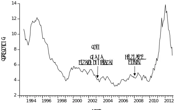
Markets and investors became myopic regarding each country’s risk and interest rates started to decline, as Figure 2 depicts for Portugal:

2

FIGURE 2 ‐ Long‐term Interest Rate for Convergence Purposes for Portugal (1993‐2012)  Source: European Central Bank.  2 4 6 8 10 12 14 1994 1996 1998 2000 2002 2004 2006 2008 2010 2012 PE R C EN TA G E YEAR Euro End of Crédito Bonificado Financial Crisis

The Portuguese banking sector took advantage of these years of low interest rates and started to get financing in international financial markets in order to keep up with and stimulate households’ housing demand, since the domestic resources were not enough to properly sustain the credit granted - a situation explored in chapter 5.

The interest rate decrease along with the liberalisation and increase of bank competition extended the access to credit to a broader group of households than in previous decades (Farinha, 2007). Portuguese families had economic growth perspectives and were able to invest in real estate, even with a modest income.

Another implication regarding the housing sector must be seriously taken into account and it regards the private renting sector. According to Associação Lisbonense de Proprietários (2011), the first legislative action towards a rent freeze was in November 1920 and in the eve of the April 25th Revolution in 1974 some rents in

Even though some measures had been taken to change the situation, the private renting sector continued to have restrictions and due to a long rent freeze there was not a considerable housing supply. Landlords simply did not find attractive to rent their properties and on top of it rents that had been updated were sometimes higher than the monthly instalments households would pay if buying their own houses.

In a time when interest rates were decreasing and banks were willing to give generous mortgage loans, the families got into debt and bought their own house and some households even invested in a second home. And this is the primarily cause of the Portuguese households’ indebtedness. Considering the private renting sector’s supply restrictions and the low interest rates, some argue that households were strangely forced to get into debt in order to get a proper housing facility at a reasonable price.

Portugal became a nation of homeowners. Also according to Associação Lisbonense de Proprietários (2011), by 2001 75% of the housing facilities were actually occupied by its own owner, comparing with 1987 where it was 57%. And the number of tenants decreased from 39% in 1981 to 21% in 2001.

Flash-forward to 2010, the economic environment is drastically different. With the 2008’s financial crisis the former myopic investors became extremely aware of the fact that the single currency does not mitigate each country’s risk. The interest rate convergence that once existed simply disappeared.

As shown in Figure 2, the long-term interest rate had an exponential increase from 2010 with the beginning of the sovereign debt crisis until approximately 2011. Not being able to deal with the interest rate increase and the unstable economic environment, in May 2011 Portugal had to ask for the IMF help for the third time,

which explains the interest rate decline at least until 2012. Having said that, the last three years have been difficult for the Portuguese families who are indebted and it is unfortunately common to hear about families who simply can no longer pay their dues.

4 | THE RATIO AS AN INDICATOR 

Financial stability has been at the heart of the authorities’ concerns since 2008 when the financial crisis struck the financial system and the most developed economies. It highlighted the need for stable financial markets and a sound banking sector and also the need for a high quality buffer to aid banks in more unstable times. As Shin (2013) states, “finding a set of early warning indicators that can signal the vulnerability to

financial turmoil has emerged as a policy goal of paramount importance in the

aftermath of the global financial crisis.”

To help national authorities on how to intervene when financial distress is a concern, the BCBS has drawn procedures to guide national authorities that use the countercyclical capital buffer regime. The BCBS is composed of more than twenty countries and provides a forum that strives for cooperation on banking regulation and supervision worldwide in order to improve and enhance financial stability.

It requires the analysis of private sector credit- to-GDP gap as it is considered a good indicator for the financial stability or “early warning indicator”. The buffer aims at protecting the banking sector from the credit cycle, i.e. from periods when credit has an excessive growth and are usually associated with riskier behaviours that may compromise financial stability.

There is also the concern to keep the banking sector solvent, stable and protected against possible future losses since its weaknesses rapidly and vastly spill over to the real economy. Banks are the link between savers and investors and are vital for companies and Governments who, on a daily basis, depend on credit to carry on their activities.

To determine whether the sector is strong or not, indicators must be used and the question lies on which one authorities should rely on. Therefore the aggregate private sector credit-to-GDP gap was determined as a common starting point. It is the difference between the credit-to-GDP ratio and its own long-term trend3 and it requires

using the HP-filter.

Other indicators are suggested by BCBS to complement this reference tool, such as real GDP growth, credit condition surveys, funding spreads and CDS spreads, among others. It is also important to be aware of the importance of the GDP behaviour since it is the denominator of the ratio used as a common reference.

However, this BCBS approach is not criticism bullet-proof. Gersl & Seidler (2011) argue that the HP-filter approach is not the most suitable for the Central and Eastern European countries since the rapid credit growth these countries had could simple mean a convergence process to the advanced economies. The authors present an estimation of those countries’ equilibrium private credit levels as an alternative indicator for excessive credit growth. Shin (2013) examines the power of three classes of early warning indicators in signalling vulnerabilities to crises. The author concludes that market prices-based indicators are unlikely to succeed and the most promising ones

3

regard banking sector liability aggregates because it can be used in real time. Regarding the credit-to-GDP ratio gap there are doubts about its ability to be used in real time. Kelly et al (2011) also raises doubts regarding the success of the indicator for countries who had a rapid credit build-up and focus the analysis in the Irish case. The authors suggest a Markov Switching framework to analyze the periods when the credit-to-GDP ratio was stable in order to analyze the long-term trend in those periods. On the other hand, Giese et al (n.d.) were able to show that the BCBS approach works for the UK and has provided sound signals of financial crises.

The contrast of these results may indicate that the BCBS proposal is not the best one for countries who had a rapid build-up in credit – such as Portugal, Ireland and Central and Eastern European countries - but it is suitable for more advanced economies, such as the UK.

In fact, BCBS points out that this indicator should only be considered as a common reference and a starting point for national authorities to make decisions. The committee also advises authorities for the need of reasoning and judgment when analyzing it in order not to be used as a mathematically indicator in decision making.

Despite the criticism, some authors have confirmed the importance of the credit-to-GDP ratio as an early warning indicator. Jordá et al (2010) show that credit growth is a good indicator for financial instability and the relation between credit growth and current accounts has becoming tighter. Drehmann et al (2011) show that the gap of the credit-to-GDP ratio is a good indicator for the build-up phase - the phase when credit growth is considerable – and it does not send too many false signals regarding the imminence of a crisis. Other indicators, such as credit growth and equity price growth,

the release phase, Drehmann et al (2011) show that market-base indicators are the ones that signal the beginning of a crisis better even though their performance is by far worst than the performance of the indicators in the build-up phase. Drehmann et al (2010) show that the difference between credit-to-GDP ratio and its long-term trend seems to be the best indicator for the build-up phase but authorities can not rely on this indicator entirely without taking into account some reasoning and judgment regarding each situation. Drehmann (2013) concludes that the gaps of bank and total credit-to-GDP ratios are good early warning indicators and may help in the countercyclical capital buffer regime.

Modern economies rely heavily on credit and it is crucial for a country to be aware of these early warning indicators. An indicator that can measure, to some extent, financial instability is a great reference but it should be considered as what it actually is, a reference. National authorities should not use this indicator or any other indicator as a mathematical rule and should always complement their decisions with judgment and discretion.

5 | EMPIRICAL ANALYSIS 

The empirical analysis of this thesis is based on Kelly et al (2011), who analyze the steady-state relationship between credit and GDP for Ireland. Considering the similarities between Ireland and Portugal as small and open economies with significant high levels of indebtedness among households, it seemed appropriate to do the same analysis for the Portuguese case.

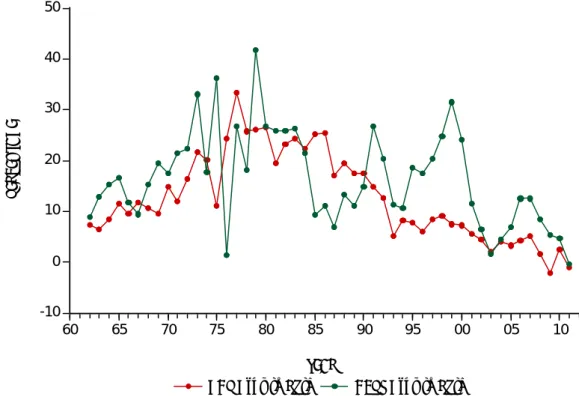
FIGURE 3 ‐ Annual Portuguese GDP and DCPS Growth Rates (1961‐2011)  Source: World Development Indicators.  -10 0 10 20 30 40 50 60 65 70 75 80 85 90 95 00 05 10

GDP Growth Rate DCPS Growth Rate

PE R C EN TA G E YEAR

Since the empirical analysis of this paper lies on the relationship between GDP and DCPS from 1961 to 2011 for the Portuguese economy, it is worth showing the annual growth rates of these variables over that period, as Figure 3 illustrates:

The GDP and DCPS annual growth rates do not exhibit a hugely correlated behaviour. Even though from 1961 to around 1973 the rates seem correlated (GDP grows and DCPS also grows), from 1973 to around 1989 the growth rates display a different behaviour. Due to the April 25th Revolution, the two IMF programmes that

Portugal had gone through and the country’s entrance in the EEC, DCPS growth is lower than GDP growth in certain years.

However, from 1990 onwards the DCPS growth rate in substantially higher than GDP growth (except for 2003 and 2011) due to the decrease of interest rates that began

during the 1990’s that encourage the increase in credit, particularly to meet the households’ housing demand.

5.1 |

METHODOLOGY AND DATA 

As previously mentioned, the econometric approach is entirely based on Kelly et al (2011). First, there is a two-state Markov Switching model to perform a structural break analysis of the DCPS-to-GDP ratio. It is a widely used model and one of its advantages is to allow observing multiple states in a relationship. The model takes the form, (1) 2 ) ( 1 ) ( 2 1             t s t s GDP DCPS t  

where s(t) is the state the economy is in at time t. A Markov chain determines s(t) and depends on a transition matrix4 which, as Kelly et al (2011) states, “gathers the

probabilities that one particular state is followed by another particular state” and “are assumed to be stationary”. The two states may be interpreted as one being a stable state and another being an unstable state - this topic is addressed in the next sub-chapter.

After making the structural break analysis there is a Granger Causality Test in order to give a hint regarding the ability of each variable to predict the other. This test will cover the entire period (1961-2011) and the sub-periods that resulted from the structural break analysis.

4

Then it follows long-run regressions to understand the relationship between DCPS and GDP not only throughout the entire period but also in the sub-periods detected. In the interest of robustness, two long-run estimators were used: the OLS (Ordinary Least Squares) and the DOLS (Dynamic Ordinary Least Squares).

The first method estimates parameters by minimizing the sum of squared residuals and it takes the following forms, depending on which variable is the independent one,

(2) GDPt 0 1DCPSt t

(3) DCPS_t ₀ ₁GDP_t _t

where ₀ is a constant term, ₁ measures the effect of the independent variable on the

dependent variable and  is the error term.

The second method is the one by Stock & Watson (1993). The DOLS purpose is to determine the long-run relationship between the variables. This method not only adds lags and leads of the differenced regressors to address autocorrelation problems but also allows for potential endogeneity between the variables. This method is also used in models regarding credit and households. Hansen & Sulla (2013) use DOLS to determine the long-run relationship between variables in a model that aims to clarify if credit growth in Latin-America is excessive and leading to a credit boom or not. Rubaszek & Serwa (2012) use DOLS in the interest of robustness to estimate the long-run relationship between the model’s explanatory variables in order to study the households’ credit behaviour over time.

Depending on the dependent variable, the DOLS regressions take the following form,

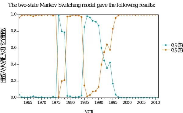
FIGURE 4 ‐ State Probabilities of the DCPS‐to‐GDP Ratio for Portugal (1961‐2011)   0.0 0.2 0.4 0.6 0.8 1.0 1965 1970 1975 1980 1985 1990 1995 2000 2005 2010 P(S(t)= 1 ) P(S(t)= 2 ) Fi lt er ed  Re gi m e  P ro b ab ilit ie s YEAR (4)   





where 0 is the constant term,  measures the effect of the independent variable 1

on the dependent variable,  is the error term and _1j measures the effect of the independent variable in first differences on the dependent variable. Since this thesis considers Kelly et al (2011) approach, it is assumed that  follows an AR(2) process and the number of leads and lags, k, is equal to 2.

Finally, all data is from the World Bank’s World Development Indicators database and covers the period from 1961 to 2011.

5.2 |

MARKOV SWITCHING MODEL 

Before entering into the analysis of the reasons that may have triggered the switches, it is required to explain both states presented in the model. State 1 is considered the unstable state since it occurs in the years when the DCPS-to-GDP ratio has quick oscillations and an erratic behaviour. Stable 2 is considered the stable state and it mainly occurs during 1961-1975 and 1992-2011 sub-periods when the ratio has a stable behaviour in the sense that grows continuously throughout.

The first switch observed is around 1975 and it may correspond to the April 25th

Revolution that released Portugal from a more than 40-year dictatorial regime. The country was in a political, social and economical turmoil and from 1974 to 1975 the ratio actually increased fifteen percentage points to return in 1976 to the same level as in 1974. According to Lopes (1982), the annual average of the 6-month credit interest rate was 7.5% in 1974 and 9,3% in 1975. This extreme increase in only one year and the already troubling economic environment may have motivated the first switch.

As explained in chapter 3, the 1970’s were a rough decade. In 1978 Portugal agreed on the first IMF programme to cope with the economical turmoil it was in and it actually corresponds to the second switch. According to Lopes (1982), the annual average of the 6-month credit interest rate was 10% in 1976, 13,3% in 1977 and by 1978 it was already 18,8%. In this programme there were quantitative limits to credit and one important goal was for national monetary authorities to keep the monetary base evolution under strict surveillance.

The third switch is around 1985 and it probably corresponds to the end of the second IMF programme that began in 1983, which also established quantitative limits to credit. The goal was to improve the balance-of-payments and to slow down inflation.

reached 28,1%, which is clearly unbearable and was one of the problems that justified the second IMF intervention.

As explained in chapter 3 Portugal joined the EEC in 1986 and when in 1992 the first steps towards a monetary union were taken the interest rates started to decline, as Figure 3 shows, and ultimately led to an increase in home-ownership by Portuguese households. In fact, the fourth and last switch is around 1992, which may correspond to the signing of the Maastricht Treaty that ultimately led to this decline in interest rates and consequently the increase of indebtedness. When analyzing the DCPS-to-GDP ratio, depicted in Figure 1, it is clear that from 1992 to 2011 the ratio increases drastically, from approximately 53,3% in 1992 to 192,1% in 2011.

5.3 |

LONG‐RUN ESTIMATES 

From the Markov Switching results two important structural breaks stand out around 1975 and 1992. For these two periods, 1961-1975 and 1992-2011, the long-run relationship between the variables was analysed carefully.

First, there is the Granger Causality Tests5. For the entire period studied and also

for the 1992-2011 sub-period GDP seems to be helpful in predicting DCPS and vice-versa. However, in the 1961-1975 sub-period GDP is said to be Granger-caused by DCPS but the opposite does not occur.

5

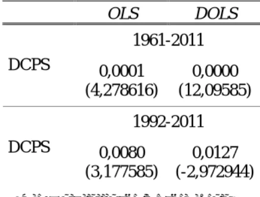
When considering the entire period, both OLS and DOLS6 estimates show that

GDP explains DCPS and vice-versa. However, when analyzing the two sub-periods closely the results are different. In the first sub-period (1961-1975) both variables are non-stationary and cointegrated, which means they have to be analysed in a Vector Error Correction (VEC) model7, which is given by the following form,

(6)

(7)

where GDP and DCPS are GDP and DCPS in first difference, respectively,

GDP

 and DCPS are the error-correction coefficients, GDP t

v and vtDCPS are the error terms,

and the expressions in parenthesis are the cointegrating vector between the variables. The results from equation (6) show the existence of short-run causality coming from DCPS to GDP but the ones from equation (7) do not show the existence of short-run causality coming from GDP to DCPS. It may be explained by the fact that throughout this period DCPS growth had an erratic behaviour that did not match the GDP growth. It is clear how DCPS grew significantly particularly in 1969, 1973 and 1975 while GDP did not. In fact, for instance, in 1975 DCPS grew 36% while GDP only grew 1%. 6 See Appendix E. GDP t t t GDP t DCPS GDP t GDP GDP GDP t v DCPS GDP DCPS GDP GDP               ) ( _{1 0 1 1} 1 1 , , 1 1 , , 0 ,       DCPS t t t DCPS t DCPS DCPS t GDP DCPS DCPS t v DCPS GDP DCPS GDP DCPS               ) ( 1 0 1 1 1 1 , , 1 1 , , 0 ,      

Another detail in equation (7) is that _DCPS is negative and statistically significant8, which means that there is a long-run causality from GDP to DCPS, i.e.

GDP causes DCPS in the long-run. In short, GDP causes DCPS in the long-run but not in the short-run.

The sub-period between 1992 and 2011 also reveals interesting results. Even tough the OLS method shows that GDP and DCPS explain each other, the DOLS approach does not show that GDP explains DCPS. And since DOLS is considered a more robust and improved method, this final result will be taken seriously into account because it may be capturing some effects that OLS is not.

It must be noticed that the Granger Causality Test results seem to contradict the OLS and DOLS results. In the first sub-period, GDP does not granger-cause DCPS and the VEC model actually does not show short-run causality coming from GDP to DCPS. However, in the second sub-period where GDP and DCPS seem to be helpful in predicting each other, DOLS shows that GDP does not explain DCPS. As mentioned previously, the Granger Causality Test aim was only to give a hint about the ability of each variable to predict each other. Despite of this possible contradiction, it is important to consider the limitations of econometric analysis since it is impossible to capture all the effects of all variables. A completely correct and flawless analysis is simply impossible.

8

5.4 |

MAIN RESULTS 

Immediately after analyzing these results there are two main conclusions.

First, for the case of Portugal, as for the case of Ireland in Kelly et al (2011), the BCBS approach does not appear to be the most suitable. Portugal clearly has two outstandingly different periods (1961-1975 and 1992-2011) that must be taken into account separately. Even though the results considering the entire period seem well-behaved it disguises the astonishing evolution this ratio has been having.

As explained in chapter 4, the BCBS approach apparently only works for economies which did not had a rapid credit build-up and our results seem to corroborate this idea. The DCPS-to-GDP ratio is an indicator of financial instability but the approach to analyse it should be taken into account carefully in order to produce the best results. As a small and open economy that had a huge credit build-up, Portugal should definitely pay attention to it in order to track the evolution of households’ indebtedness and its own financial stability.

Second, the DOLS results for the second sub-period showing that GDP does not explain DCPS may suggest a break of the link between deposits and credit. Traditionally, banks grant credit to investors and households according to the deposits made by savers and there has always been this link that had kept the banking system sound and stable. However Figure 3 shows some sub-periods where the DCPS growth rate was significantly higher than the GDP growth rate. Assuming that savings are related to a country’s economic performance and taking into account that Portugal’s GDP did not grew significantly in the past two decades, apparently credit growth was

Actually, Banco de Portugal (2004) stated that “the strong growth in credit

granted by the banking system since the mid-1990s has not been matched by similar

developments in resources from customers. In fact, deposits with the Portuguese

banking system recorded relatively moderate growth rates over the past few years”.

From approximately the 1990 decade that traditional banking conduct was not the case for the Portuguese banking sector. Due to the lack of domestic resources and a strong credit growth fuelled by households’ housing demand, banks had to resort to alternative forms to finance credit, such as the international financial markets. Banks realized that there was no longer the obligation to only grant credit with respect to deposits since they had access to an almost limitless pool of funds at a low interest rate that allowed them to do business differently. For Banco de Portugal (2004), “recourse

to market financing is relatively more important for the larger Portuguese domestic

groups than for most banks in other European countries”. And “the increasing share of

Portuguese banks’ borrowing from international financial markets increases potentially

their vulnerability to changes in the sentiment of these markets”, as Banco de Portugal

(2005) also warns.

FIGURE 5 ‐ Bank Credit to Bank Deposits Ratio (%) for Portugal (1961‐2011)  Source: World Development Indicators. 60 80 100 120 140 160 180 60 65 70 75 80 85 90 95 00 05 10 PE R C EN TA G E YEAR

Figure 5 shows the credit-to-deposits ratio and when it is above 100% it means that bank credit is higher than bank deposits i.e., bank credit is not based in proper deposits. It is probably the best exhibit of how the link between credit and deposits has been broken for a few years in Portugal.

From approximately the April 25th Revolution until 1977 the ratio increases

considerably and reaches 121%. Considering the social and political situation at the time, this increase is expected since Portugal received thousands of Portuguese people from the former colonies after the end of the regime and it was one of the causes for the first IMF intervention in the country – as explained in chapter 3.

Due to the IMF intervention in 1978 and 1983 that established quantitative limits to credit, as mentioned in chapter 5.2, from 1977 onwards and throughout the 1980 decade the ratio decreased and reached 64% in 1989, the minimum value reached in this sample.

From the 1990 decade onwards the ratio increased dramatically, reaching its maximum of 170% in 2007. The financial crisis made the credit-to-deposits ratio decline considerably from 2007 to 2010 not only because it brought financial instability but most importantly because it brought risk awareness, which made credit standards stricter. Investors were no longer myopic and the interest rates increased tremendously, as Figure 2 illustrates.

It is also worth to mention how the current account balance9 accompanies the

evolution presented in Figure 5. From around 1996 to 2008, the current account balance decreased significantly and reached -12,6% of GDP in 2008, which means that throughout this period the Portuguese economy was being financed by external savings, i.e. Portugal was living above its means. Therefore the increase in credit without a proper basis contributed to the degradation of the current account balance, which is one of the causes of the current European crisis that is dragging the Portuguese economy.

Banks’ behaviour throughout the 1990 decade and the beginning of the 2000’s has been seriously and heavily criticized for being irresponsible since they conducted a dramatic credit growth based on loose standards. The alternative forms of financing credit other than deposits were justified by a huge demand for house-ownership by households. However, banks should not have their responsibility in the situation completely removed since they encouraged this demand with attractive mortgages even for households with more a modest income.

When discussing banks’ responsibility in the current levels of households’ indebtedness it is important to point out that during those years of loose credit their

9

conduct was not stopped or questioned. Banco de Portugal, as the regulator, did not find

the situation worrisome and took no actions to prevent the exponential increase of the bank credit-to-banks deposit ratio.

Throughout the 1990’s and the beginning of the 2000’s the regulator’s attitude towards the situation has been passive and no preventive actions were taken. Nevertheless, Banco de Portugal acknowledges the high levels of households’

indebtedness and the fact that banks used the international financial markets considerably to support credit.

It would be expected that around the year of 2000 Banco de Portugal would had

noticed the already significant increase in the credit-to-deposit ratio and tried to control or diminish the situation. In spite of it, it maintained a passive attitude by assuming that there was no problem regarding financial stability because households’ debt was based on a real asset – houses - and since the institution assumes no housing bubble, there would always be an asset that banks could rely on in case of default. Banco de Portugal (2008) actually states that “financial stability should not be in jeopardy” considering

that “credit to individuals being dominated by credit for owner-occupier mortgages

helps to explain it”. It also defends “no evidence of situations of excessive valuation of

property assets in the country”.

Banco de Portugal also assumed that there would be no considerable risks to

financial stability since the most indebted households are the ones with low income and even though their participation in the debt market is high, the amounts borrowed are not significant when comparing to the total, as explained in chapter 2. Banco de Portugal (2008) stated that even though “the near future does not bode well, with an increase in

seems to be little likelihood of the situation affecting financial stability in any

substantial way.”

Considering that this was the regulator’s stance, banks basically had free rein to continue with their risky behaviour: they were not demanded to explain their behaviour and received no signs from the regulator to control the situation.

Finally, it is important not to forget that everyone contributed to this dramatic situation. Banks granted credit without a proper basis but households also got into a debt significantly high considering their income. And, most importantly, the regulator had a passive attitude towards the situation throughout the most critical years.

6 | CONCLUSIONS 

This paper analyses the reasons of the Portuguese households’ indebtedness, a topic that may not be receiving the attention it deserves considering its implications on the economy.

Since the 2008’s financial crisis it has been a growing concern for authorities to be provided with the so-called “early warning indicators” in order to be able to take prudent actions when facing financial distress. The BCBS suggests using the HP-Filter to determine the Private Sector credit-to-GDP gap i.e., the difference between the credit-to-GDP ratio and its own long-term trend, and recommends it as a common starting point for authorities to determine whether there is an excessive credit growth or not.

This approach is not bullet-proof and some authors have shown that it is not the most appropriate for countries that have experienced a rapid credit build-up. Kelly et al (2011) reached the same conclusion for the case of Ireland, a small and open economy. Due to the similarities with Portugal, this paper uses Kelly et al (2011) empirical analysis to determine if the BCBS approach is the most appropriate or not.

With World Development Indicators data of the DCPS-to-GDP ratio from 1961 to 2011, a two-state Markov Switching model was constructed to explore the structural breaks the ratio may have and the periods where long-run estimates could be made. There were two major structural breaks that showed two important sub-periods: 1961 to 1975 and 1992 to 2011. The long-run relationship between DCPS and GDP was analyzed in these sub-periods as well in the entire period using OLS and DOLS methods.

There are two main conclusions. The first one is that BCBS approach is not the most suitable for the case of Portugal because it disguises the existence of two outstandingly different periods, particularly the second one.

The second main conclusion is that GDP does not explain DCPS from 1992 to 2011, which probably indicates that the link between deposits and credit has been broken in this sub-period. Banks started to get financing in international financial markets in order to satisfy the particularly strong households’ housing demand which, in fact, was partly encouraged by banks with attractive mortgages even for households with a more modest income. Even though the banking sector had an irresponsible conduct, it was not stopped or prevented by Banco de Portugal who assumed a passive

The dramatic evolution of Portugal’s DCPS-to-GDP ratio was a considerably loud “early warning indicator” that was not seriously taken into account by authorities. It encouraged the Portuguese bank’s daring behaviour during the 1990’s and beginning of the 2000’s and fuelled a tremendous credit build-up that ultimately damaged the country’s financial stability.

7 | REFERENCES 

Associação Lisbonense de Proprietários, (2011). Retrato da Habitação em Portugal:

característica e Recomendações. Associação Lisbonense de Proprietários.

Banco de Portugal, (2004). Financial Stability Report 2004. Banco de Portugal.

Banco de Portugal, (2005). Financial Stability Report 2005. Banco de Portugal.

Banco de Portugal, (2008). Financial Stability Report 2008. Banco de Portugal.

Basel Committee on Banking Supervision, (2010). Guidance for national authorities

operating countercyclical capital buffer. Bank for International Settlements.

Costa, S. and Farinha, L. (2012). Households' indebtedness: a microeconomic analysis

based on the results of the households' financial and consumption survey.

Financial Stability Report 2012. Banco de Portugal, pp.133-157.

Costa, S. (2012). Households' default probability: an analysis based on the results of

the HFCS. Financial Stability Report 2012. Banco de Portugal, pp.97-110.

Castro, G. (2006). Consumption, disposable income and liquidity constraints. Economic

Dgtf.pt, (n.d.). Direcção Geral do Tesouro e Finanças. [online] Available at:

http://www.dgtf.pt/estatisticas/credito-a-habitacao/indicadores [Accessed 2 May. 2014].

Drehmann, M., Borio, C. and Tsatsaronis, K. (2011). Anchoring countercyclical capital buffers: the role credit aggregates. Bank for International Settlements, (355).

Drehmann, M., Borio, C., Gambacorta, L., Jiménez, G. and Trucharte, C. (2010). Countercyclical capital buffers: exploring options. Bank for International

Settlements, (317).

Drehmann, M. (2013). Total credit as an early warning indicator for systemic banking crises. BIS Quaterly Review, pp.41-45.

Farinha, L. and Noorali, S. (2004). Indebtedness and wealth of Portuguese households.

Financial Stability Report 2004. Banco de Portugal, pp.131-143.

Farinha, L. (2007). Indebtedness of Portuguese households: recent evidence based on

the household wealth survey 2006-2007. Financial Stability Report 2007. Banco de

Portugal, pp.129 - 152.

Gersl, A. and Seidler, J. (2011). Excessive credit growth as an indicator of financial

(in)stability and its use in macroprudential policy. Financial Stability Report

2010/2011. Czech National Bank, pp.112-122.

Giese, J., Andersen, H., Bush, O., Castro, C., Farag, M. and Kapadia, S. (n.d.). The credit-to.-GDP gap and complementary indicators for macroprudential policy: evidence from the UK.

Hansen, N. and Sulla, O. (2013). Credit growth in Latin-America: financial development or credit boom?. International Monetary Fund.

Jordá, Ò., Schularick, M. and Taylor, A. (2010). Crises, Credit Booms and External Imbalances: 140 years of lessons. National Bureau of Economic Research,

(16567).

Kelly, R., McQuinn, K. and Stuart, R. (2011). Exploring the steady-state relationship

between credit and GDP for a small open economy – the case of Ireland. Central

Bank of Ireland.

Lopes, J. (1982). IMF conditionality in the stand-by arrangement with Portugal of 1978.

Estudos de Economia, III(2), pp.141-166.

Pinto, A. (1983). A economia portuguesa e os acordos de estabilização económica com o Fundo Monetário Internacional. Economia, VII(3), pp.555-596.

Rubaszek, M. and Serwa, D. (2012). Determinants of credit to households in a life-cycle model. European Central Bank, (1420).

Shin, H. (2013). Procyclicality and the Search for Early Warning Indicators. In:

Financial Crises: Causes, Consequences and Policy Response. International

Monetary Fund.

Stock, J. and Watson, M. (1993). A simple estimator of cointegrating vectors in higher order integrated systems. Econometrica, 61(4), pp.783-820.

Source: Kelly et al (2011). 

Source: Direcção Geral do Tesouro e Finanças.

Appendix A | FIGURE 6 ‐ Select European Countries Levels of Financial Deepening 

(1999−2010) 

Source: Author’s calculations. Note: Tests conducted with 2 lags. The F‐statistics are in parenthesis.  Source: Author’s calculations.  Appendix C | TABLE I ‐ Constant Markov Transition Probabilities Matrix  j) /column i (row ) ) 1 ( | ) ( ( ) , (      P s t k s t i k i P       Appendix D | TABLE II – Granger Causality Tests        1 2 1 0.769918 0.230082 All periods 2 0.049433 0.950567 1961-2011 1961-1975 1992-2011 GDP does not Granger Cause

DCPS 0,0005 (9,17808) 0,0096 (8,764) 0,022 (5,1929)

DCPS does not Granger Cause GDP 0,0003 (9,87126) 0,2789 (1,50441) 0,0081 (7,14392)

TABLE III  LONG‐RUN ESTIMATES OF PORTUGUESE GDP  Note: T‐statistics are in parenthesis. Source: Author’s calculations. TABLE IV  LONG‐RUN ESTIMATES OF PORTUGUESE DCPS  Note: T‐statistics are in parenthesis. Source: Author’s calculations. Appendix E | Long‐run Estimates    OLS DOLS 1961-2011 DCPS _0,0001 (4,278616) 0,0000 (12,09585) 1992-2011 DCPS _0,0080 (3,177585) 0,0127 (-2,972944) OLS DOLS 1961-2011 GDP _0,0001 (4,278616) 0,0001 (4,33752) 1992-2011 GDP _0,0080 (3,177585) 0,6398 (-0,481195)

Note: T‐statistics are in parenthesis. Source: Author’s calculations. Note: T‐statistics are in parenthesis. Source: Author’s calculations. Appendix F | TABLE V – Vector Error Correction (VEC) Model   Appendix G| TABLE VI – VEC Model: Error‐correction Coefficients  Dependent Variable GDP DCPS DCPS 0,0151 (2,994773) GDP 0,5824 (-0,570335) Error-correction Coefficients GDP DCPS GDP  -0,159536 (0,4019) DCPS  -72,56581 (0,0009)

Source: International Monetary Fund. -16 -12 -8 -4 0 4 80 82 84 86 88 90 92 94 96 98 00 02 04 06 08 10 PE R C EN TA G E YEAR Appendix H | FIGURE 8 – Current Account Balance as % of GDP (1980−2011)  Appendix I | FIGURE 9 – Comparison between Current Account Balance and the Bank  credit‐to‐ Bank deposits Ratio  Source: International Monetary Fund and World Development Indicators.  -40 0 40 80 120 160 200 60 65 70 75 80 85 90 95 00 05 10 Cur rent Account Balance Bank Credit to Bank Deposits ratio PE R C EN TA G E YEAR