Efficient Operations at Intermodal Terminals Using a Multi-agent System

Using a Multi-agent System

Tomás Hipólito, João Lemos Nabais and Miguel Ayala Botto

Abstract Transport networks are large-scale complex systems whose objective is to deliver cargo at a specific time and at a specific location. Ports and intermodal container terminals behave as exchange hubs where containers are moved from a transport modality to a different one. Terminal operations management arise as a need to face the exponentially growth of the container traffic in the last few years. In this paper the Extended Formulation of the MPC is presented. This formulation accounts for the variation of the control action to reduce not only the amount of actions but to perform a wise and efficient use of handling resources. This formula-tion is based on the decomposiformula-tion of the control acformula-tion. The Extended Formulaformula-tion is applied to a simulation case study based on a long-term scheduled scenario and compared with the Basic Formulation.

Keywords Model Predictive Control

⋅

⋅

⋅

⋅

1

Introduction

The container emerged in 1950s as solution to transport goods over long distances. Container transportation networks are designed to deliver cargo at the agreed time and at the agreed location. Intermodal container terminals behave as exchange hubs where containers are handled, eventually stored or moved to other transport modality to reach the final destination at the agreed time. The need for operations management at intermodal container terminals arise from the need to offer effective and efficient processes which meet the network requirements, while minimizing operating costs

T. Hipólito⋅ M.A. Botto

LAETA, IDMEC, Instituto Superior Técnico, Universidade de Lisboa, Lisboa, Portugal

J.L. Nabais (

✉

LAETA, School of Business Administration, IDMEC, Polytechnical Institute of Setúbal, Setúbal, Portugal

e-mail: joao.nabais@esce.ips.pt

© Springer International Publishing Switzerland 2017 P. Garrido et al. (eds.),CONTROLO 2016, Lecture Notes

in Electrical Engineering 402, DOI 10.1007/978-3-319-43671-5_14

[1]. The productivity of an intermodal terminal and thus of a network can be sig-nificantly improved by suitably modelling and optimizing the handling of terminal resources [2]. The operations management related to intermodal containers terminals can be analysed as a flow assignment problem, where the container flows are guaran-teed by the allocation of the handling resources. The efficiency of a terminal is influ-enced by the ability to manage the transfer processes performed by the resources [2]. The operations management at container terminals has been widely studied by the operations research field [3–6]. These approaches focus on the optimization of indi-vidual terminal operations such as berth planning and container storage. However, they lack a general approach considering all terminal operations simultaneously. The control field has also done research in this area applying classic control techniques and assuming undistinguished containers [2, 7, 8]. The ability to distinguish con-tainers is relevant to network operation because it creates the possibility to group them according their features. Containers can be distinguished according to some relevant criteria: weight, size, due time, final destination. More recently, a new con-trol approach was developed considering Model Predictive Concon-trol (MPC) technique and distinguishable containers [9–11]. MPC is suitable for large dimensional prob-lems with multiple variables and it has been used with success in petrochemical and electromechanical industry [12]. These approaches consider the control action as the decision variable intended to minimize. In MPC problems the cost function penal-izes changes in the variation of the control action rather than the control action itself [12]. In terms of the terminal, variation of control action corresponds to the varia-tion of the allocavaria-tion of handling resources and the objective is to minimize it. In this paper, the container terminal is modelled from a push-pull container flow perspec-tive. The model is used to develop a decomposition of the general flow assignment problem into subproblems which are handled by MPC control agents [9]. The main contribution of this paper is:

∙ formulation of the optimization problem considering the variation of control action𝜟u which focus on the variation of the utilization of handling resources. In Sect.2the intermodal container terminal model is presented considering a generic framework that is able to capture different structural layouts. The control structure is presented in Sect.3. For comparison purposes the optimization problem is formu-lated considering the control action u, Basic Formulation (Sect.3.1) and the variation of control action𝜟u, Extended Formulation (Sect.3.2). In Sect.4numerical results are presented, in which Extended Formulation is compared to Basic Formulation.

2

Background

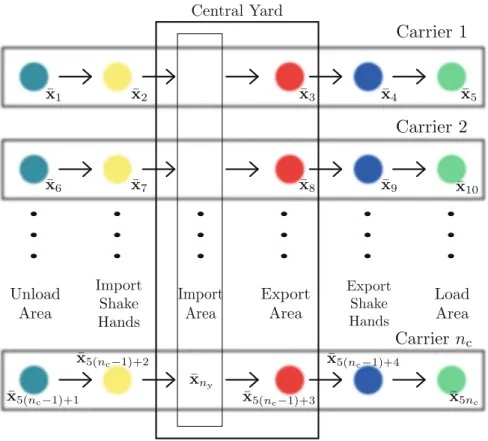
The intermodal container terminal can be represented by a graph = (, ), where the nodes stand for the storage areas and the links  refer to the container flows between nodes (Fig.1). The model describing the terminal dynamics is based on a flow perspective and it assumes two main concepts:

Fig. 1 Intermodal container terminal graph considering naexclusive areas per connection plus a common node for all connections

∙ storage areas—to model the storage capacity of terminal physical areas.

∙ container categorisation—to distinguish containers according its final destination and track them inside the terminal.

The model assumes that the terminal is split into five main areas (see Fig.1): ∙ Unload Area—area related to the unloading of containers from the carriers to the

terminal.

∙ Import Shake Hands—area connecting the Unload Area to the Central Yard where occurs a handling resource switch.

∙ Central Yard—core of the container terminal. It is divided into Import Area where the containers are stored and Export Area where the containers prepared to be exported.

∙ Export Shake Hands—area connecting the Central Yard and the Load Area where occurs a handling resource switch.

∙ Load Area—area related to the loading of containers from the terminal to the carriers.

For each connection arriving the terminal a container flow is established based on the movement of the containers promoted by handling resources from Unload Area to the Central Yard and from the Central Yard to the Load Area. The topology of the model depends on the following parameters: number of different container classes present in the terminalntwhich is related to the number of possible final destinations; number of connections provided by the terminal simultaneouslyn_c, which can be of different transport modalities; number of storage areas exclusive of a single connec-tionn_a. The intermodal container terminal hasn_ctransport connections (see Fig.1). The model considers each connection as a subsystem and a control agent is assigned to each subsystem. The subsystems have coupled dynamics because they share a common node, the Import Area of the Central Yard, and coupled constraints because connections share the handling resources available. Mathematically the model of ter-minal is formulated using a state-space approach. There are n_cstate space vectors x_i, wherei = 1 … n_c. Each state space vector x_iis composed of the correspondinḡx_j state space vectors associated to the subsystemi specific nodes plus the state of the common node. x_i(k) = ⎡ ⎢ ⎢ ⎢ ⎢ ⎣ ̄x_n Ai+1(k) ⋮ ̄x_n Ai+nai(k) ̄x_ny(k) ⎤ ⎥ ⎥ ⎥ ⎥ ⎦ , nA_i = i−1 ∑ j=1 na, 1 ≤ i ≤ nc (1)

Each state space vector x_i belongs to the state space set i and its length is (na+ 1)nt. The state-space model for subsystemi is given by

x_i(k + 1) = A_ix_i(k) + B_u,iu_i(k) + B_d,id_i(k) + nc ∑ j=1,j≠i B_u,iju_j(k) (2) y_i(k) = C_ix_i(k) (3) x_i(k) ≥ 0 (4) u_i(k) ≥ 0 (5) y_i(k) ≤ y_max,i (6) P_uu,iu_i(k) ≤ u_max,i (7) x_i(k) ≥ P_xu,iu_i(k) (8) x_i(k) ∈ i (9) u_i(k) ∈ i (10)

where vector u_i(k) represents the control action for subsystem i and its length is n_an_t, vector d_i(k) stands for the perturbation (arrival and departure of containers) in sub-systemi and its length is 2n_t, y_i(k) is the amount of containers present at the physical areas of subsystemi. Vectors y_max,iand u_max,icorrespond to the maximum amount of containers possible at the terminal areas and to the maximum handling capacity

of subsystemi. Matrices A_i, B_u,i, B_d,i, B_u,ijand C_iare the state space matrices for subsystemi. P_uu,iis the projection matrix from the control action set i into the maximum handling capacity set_maxi , P_xu,iis the projection matrix from the control action setiinto the state space seti.

3

Control

MPC is particularly suited to deal with terminal operations management since it is able to operate near the constraints limits, namely, the handling capacity and the stor-age capacity and perform the optimization of large dimensional problems as this one [12]. MPC has already been adopted successfully to control large and multi-variable processes in the industry [13, 14], structurally similar to the terminal operations management problem. The control goal is to perform an efficient flow assignment in order to increase the terminal performance according to a pre-defined parameter. The minimization of terminal operation costs is a desired goal which can be achieved by minimizing the amount of handling resources actions.

3.1 Basic MPC Formulation

The objective of the Basic Formulation is to minimize the control action u(k) while fulfilling the transport network requirements. At each time step, the controller finds the minimum amount of containers necessary to move in order to satisfy termi-nal constraints. The objective function for subsystem i is linear and consists on a weighted sum of the storage areas

J(k) =N−1∑ j=0

qT_p,ix_i(k + 1 + j) (11)

where q_p,icorrespond to the weights assigned to the storage areas. Combining (2) with (11), objective function is written in terms of the decision variable u_i(k)

J(k) = N−1_∑ j=0 qT_p,i[A_ix_i(k + j) + B_u,iu_i(k + j) + B_d,id_i(k + j) + nc ∑ j=1,j≠i B_u,iju_j(k)] (12)

The Basic MPC formulation for control agenti which is responsible for subsystem i is presented as: min ̃ui Np−1_∑ j=0

qT_p,i[A_ix_i(k+j)+B_u,iu_i(k+j)+B_d,id_i(k+j)+ nc

∑ j=1,j≠i

B_u,iju_j(k)] (13) s.t. x_i(k+1+ j)=A_ix_i(k+j)+B_u,iu_i(k+j)+B_d,id_i(k+j)+

nc ∑ j=1,j≠i B_u,iju_j(k) (14) y_i(k + j) = C_ix_i(k + j), j = 0, … , N_p− 1 (15) x_i(k + j) ≥ 0 (16) u_i(k + j) ≥ 0 (17) y_i(k + j) ≤ y_max,i (18) P_uu,iu_i(k + j) ≤ u_max,i (19) x_i(k) ≥ P_xu,iu_i(k + j) (20) P_dx,ix_i(k + 1 + j) ≤ w_d,i(k + 1 + j) (21) whereN_pis the prediction horizon, ̃u_iis the control action sequence over the predic-tion horizon[u_i(k)T _{… u}

i(k + Np− 1)T ]T

, vector wd,i(k) represents the forecast load request vector for subsystemi that is updated at each time step k and matrix Pdx,i is the projection matrix from the state space setiinto the load request set of sub-systemi. The constraints are included in the optimization problem formulation to assure a meaningful terminal behaviour over the time. Equations (16) and (17) guar-antee the non-negativity of the states, because it is not physically possible to have a negative storage in the nodes and the non-negativity of the control actions, which is a necessary condition to have a coherent model. Equation (18) imposes a storage capacity limit to each physical area of the terminal that needs to be respected because it is an inherent characteristic of the terminal. Equation (19) indicates that the con-trol actions must respect the maximum handling capacity of the terminal resources. Equation (20) assures that is only possible to move containers from one node to another if there are effectively containers in those nodes. Equation (21) expresses the load request imposed by the clients. Control agents are solved sequentially according a pre-determined order. It is possible to choose any agent order at the beginning of the simulation but that order is constant. The MPC controller updates the state of the Import Area of the Central Yard and the resources available after solving a control agent.

3.2 Extended MPC Formulation

The objective of the Extended Formulation is to minimize the variation of the con-trol action𝜟u(k) while fulfilling the transport network requirements. At each time

step, the controller allocates the resources keeping the flows constant between nodes. Using this approach and considering an ideal situation handling resources are being fully used or not used at all. This formulation is focused on the efficiency of the usage of handling resources which is desirable to reduce operation costs. Extended Formulation rewrites control action vector of subsystemi u_i(k) as:

u_i(k) = 𝜟u_i(k) + u_i(k − 1) (22) The Extended MPC formulation for control agenti which is responsible for subsys-temi is stated as:

min ̃ui(k) N−1_∑ j=0 qT_p,ix_i(k + 1 + j) (23) s.t. x_i(k + 1 + j) = A_ix_i(k + j) + B_u,i[𝜟u_i(k + j) + u_i(k − 1 + j)]+ B_d,id_i(k + j) + nc ∑ j=1,j≠i B_u,iju_j(k) (24) y_i(k + j) = C_ix(k + j), j = 0, … , N − 1 (25) x_i(k + j) ≥ 0 (26) [𝜟u_i(k + j) + u_i(k − 1 + j)] ≥ 0 (27) y_i(k + j) ≤ y_max,i (28)

P_uu,i[𝜟u_i(k + j) + u_i(k − 1 + j)] ≤ u_max,i (29) x_i(k) ≥ P_xu,i[𝜟u_i(k + j) + u_i(k − 1 + j)] (30) P_dx,ix_i(k + 1 + j) ≤ w_d,i(k + 1 + j) (31) To evaluate the performance of MPC controller under variable conditions and parameters Performance Metrics (PM) was designed. Performance Metrics is a metrics based on objective function. The expression, PM= qT

px(k + 1), takes into account just the control action of the current time step u(k) which corresponds to the actions that are being implemented in the terminal. This way bias effects of large control sequences are avoided.

4

Results

The presented MPC control structure will be used for controlling an hinterland ter-minal with the following layout (see Fig.2):

∙ a quay area able to berth two barges simultaneously at maximum. Containers are unloaded/loaded from/to barges by Quay Cranes. QC maximum handling capacity is 90 TEU/hour. Berth A is able to use the maximum cranes capacity, while berth B is only able to use half of the maximum cranes capacity, 45 TEU/hour.

Fig. 2 Intermodal container terminal layout for simulation purposes

∙ a train area with two rail tracks available. Containers are unloaded/loaded from/to wagons by train gates. The maximum handling capacity of the train gates is 40 TEU/hour.

∙ a truck area, where there is a maximum handling capacity of 60 TEU/hour. Focusing on storage capacity of the terminal areas, the Unload Area, the Load Area and the Central Yard are considered to be large enough to never compromise the terminal operations, so they have a storage capacity of 20000 TEU. The Import Shake Hands/Export Shake Hands are intermediate areas and are not designed to store cargo, so their storage capacities are limited to the respective unload/load max-imum capacity for each carrier: 90 TEU for Barge A, 45 TEU for Barge B, 40 TEU for train A, 40 TEU for train B, 60 TEU for trucks.

A network of connections and weekly schedules is designed to manage the container flows of the hinterland terminal. This schedule is result of agreements between all the parts involved in the management and coordination of the transportation network so it is assumed to be fixed. Some assumptions are made per transport modality: ∙ Barges: it is assumed that three connections per day will be available in a 6-day

week. An average handling of 280 TEU/demand and 120 TEU/demand for berth A and berth B, respectively, will be considered for numerical design.

∙ Trains: two rail tracks are available that serve exclusively one train. The schedule for trains is assumed fixed and four shipments per day for each rail track are avail-able for a 6-day week. An average handling of 80 TEU/demand for both trains will be considered for numerical design.

∙ Trucks: truck gates are only open for a 16 h period on a 6-day week. Every hour trucks arrive and leave the train. An average handling of 60 TEU/demand for trucks will be considered for numerical design.

The container transfer towards the Central Yard is performed by Automatic Guided Vehicles (AGV) and the rehandling of containers at the Central Yard from Import Area to the Export Area is performed by Rail Mounted Gantry Cranes (RMGC). The terminal is integrated in a transport network composed by 4 terminals, son_t= 5, including the empty containers. As stated above, the number of connections served by the terminal isn_c= 5. Each connection has 5 exclusive areas which are Unload Area, Import Shake Hands, Export Area, Export Shake Hands, Load Area, son_a= 5. The scenario corresponds to one week of terminal operation, the prediction horizon considered isN_p = 6 and the sampling time assumed is T_s= 1 h.

MPC formulations are compared using two criteria: the performance metrics and the computation time. Figures3and4reveal that the behaviour of the two formulations is similar. The Performance Metrics values (see Table1) confirm the similarity. This similarity is due to the strict structure of connections schedule. The schedule is based on time windows which are not long enough to see the effect of the variation of the control action. The Extended Formulation is justified because it consists on a tactical decision which is performed to achieve the strategic goal which can be the reduction of operational costs. In terms of computation time, Extended Formulation takes the double of the time of Basic Formulation. The decomposition of u(k) increases the complexity of Extended Formulation.

Fig. 3 Container storage at the import area considering the Basic Formulation and the Extended Formulation

k 0 10 20 30 40 TEU 8600 8800 9000 9200 9400 B.Formulation E.Formulation

Fig. 4 Quay Crane allocation considering the Basic Formulation and Extended Formulation k 0 10 20 30 40 TEU 0 20 40 60 80 100 B.Formulation E.Formulation Max.QC

Table 1 Computation time and performance metrics

MPC formulation Computation time Performance

metrics

Max [s] Mean [s] Stdv [s]

Basic 0.5304 0.3326 0.0689 −4317.2

Extended 0.8892 0.6111 0.821 −4318.4

5

Conclusions

In this paper, Extended Formulation of MPC is presented. Extended formulation consists in considering the control action variation as the decision variable of the optimization problem instead of the control action itself. The main advantage of the Extended Formulation consists on focusing on the monetization of handling resources movements instead of just minimize the amount of containers. This for-mulation introduces a tactical approach to operations management trying to meet management objectives namely cost reduction by reducing resources movements at the cost of not moving the minimum amount of containers at each time step. New terminal layouts, including more terminal areas and connections new schedules need to be tested using this formulation to validate it.

Acknowledgments This work was supported by Fundação para a Ciência e Tecnologia (FCT), through IDMEC, under LAETA, project UID/EMS/50022/2013 and by the FCT, through IDMEC, under LAETA Pest-OE/EME/LA0022.

References

1. Stahlbock, Robert, Voss, Stefan: Operations research at container terminals: a literature update. OR Spectrum 30, 1–52 (2008)

2. Alessandri, A., Sacone, S., Siri, S.: Management of intermodal container terminals using feed-back control. In: Proceedings of The 7th International IEEE Conference on Intelligent Trans-portation Systems, pp. 882–887 (2004)

3. Crainic, T.G., Kim, K.H.: Intermodal Transportation. Technol. Teach. 64, 15–18 (2005) 4. Gambardella, L.M., Mastrolilli, M., Rizzoli, A.E., Zaffalon, M.: An optimization methodology

for intermodal terminal management. J. Intell. Manuf. 12, 5–6 (2001)

5. Kozan, E., Preston, Peter: Genetic algorithms to schedule container transfers at multimodal terminals. Int. Trans. Oper. Res. 6, 311–329 (1999)

6. Legato, Pasquale, Mazza, Rina M.: Berth planning and resources optimisation at a container terminal via discrete event simulation. Eur. J. Oper. Res. 133, 537–547 (2001)

7. Alessandri, Angelo, Cervellera, Cristiano, Cuneo, Marta, Gaggero, Mauro, Soncin, Giuseppe: Modeling and feedback control for resource allocation and performance analysis in container terminals. IEEE Trans. Intell. Transp. Syst. 9, 601–614 (2008)

8. Alessandri, Angelo, Cervellera, Cristiano, Cuneo, Marta, Gaggero, Mauro, Soncin, Giuseppe: Management of logistics operations in intermodal terminals by using dynamic modelling and nonlinear programming. Marit. Econ. 11, 58–76 (2009)

9. Nabais, J.L., Negenborn, R.R., Botto, M.A.: Hierarchical model predictive control for optimiz-ing intermodal container terminal operations. IEEE Conf. Intell. Transp. Syst. Proc. 708–713 (2013)

10. Nabais, J.L., Negenborn, R.R., Botto, M.A.: A novel predictive control based framework for optimizing intermodal container terminal operations. In: 3rd International Conference on Com-putational Logistics, pp. 53–71 (2012)

11. Negenborn, R.R.: Model predictive control for a sustainable transport modal split at intermodal container hubs (2013)

12. Maciejowski, J.M.: Predictive Control with Constraints. Prentice Hall (2002)

13. Stewart, Brett T., Venkat, Aswin N., Rawlings, James B., Wright, Stephen J., Pannocchia, Gabriele: Cooperative distributed model predictive control. Syst. Control Lett. 59, 460–469 (2010)

14. Venkat, A.N., Hiskens, I.A., Rawlings, J.B., Wright, S.J.: Distributed MPC strategies with application to power system automatic generation control. IEEE Trans. Control Syst. Technol.