1
LAND COVER MAPPING WITH RANDOM
FOREST USING INTRA-ANNUAL SENTINEL
2 DATA IN CENTRAL PORTUGAL
A COMPARATIVE ANALYSIS
ii
Land cover mapping with Random Forest using intra-annual Sentinel-2
data in Central Portugal
A comparative analysis
Dissertation supervised by PhD Roberto Henriques
Professor, Nova Information Management School University of Nova – Lisbon, Portugal
PhD Mário Caetano
Professor, Nova Information Management School University of Nova – Lisbon, Portugal
PhD Carlos Grannell
Professor, Universitat Jaume I – Castellón, Spain
iii ACKNOWLEDGMENTS
I would like to thank first my supervisor and co-supervisors Roberto Henriques, Mário Caetano and Carlos Granell. Their support and guidance in the realization of this research was indispensable.
I also leave my most sincere gratitude to the professors Joaquín Huerta, Michael Gould, Marco Painho, Christoph Brox, and Christian Kray for the organisation of the Master of Science in Geospatial Technologies and the support they gave to us students over the course of the degree. I would also thank all professors involved in the program for sharing their knowledge.
A special thank you goes out to Hugo Costa, formerly employed at the DGT in Lisbon, who gave a lot of his valuable time to support me with the methodology and critical input to my work. It was a pleasure to work with you.
My appreciation also goes to NOVA IMS, who supported my journey with a scholarship for the last semester.
My classmates also deserve my gratitude, since they made this experience what it was. I am glad to call you my friends, and I hope to share more memories with you in the future. A special shout out to Mr. Chaplin Williams, who was my closest ally and working mate. I can’t imagine this journey without, and I am more than grateful for your presence and all the things I learned from you.
A final thank you to my friends and family, who were very supportive throughout the experience.
iv
ABSTRACT
In recent years, data mining algorithms are increasingly applied to optimise the classification process of remotely sensed imagery. Random Forest algorithms have shown high potential for land cover mapping problems yet have not been sufficiently tested on their ability to process and classify multi-temporal data within one classification process. Additionally, a growing amount of geospatial data is freely available online without having their usability assessed, such as EUROSTAT´s LUCAS land use land cover dataset.
This study provides a comparative analysis of two land cover classification approaches using Random Forest on open-access multi-spectral, multi-temporal Sentinel-2A/B data. A classification system composed of six classes (sealed surfaces, non-vegetated unsealed surfaces, water, woody, herbaceous permanent, herbaceous periodic) was designed for this study. Ten images of ten bands plus NDVI each, taken between November 2016 and October 2017 in Central Portugal, were processed in R using a pixel-based approach. Ten maps based on single month data were produced. These were then used as input data for the classifier to create a final map. This map was compared with a map using all 100 bands at once as training for the classifier. This study concluded that the approach using all bands produced maps with 11% higher, yet overall low accuracy of 58%. It was also less time-consuming with about 5 hours to over 15 hours of work for the multi-temporal predictions. The main causes for the low accuracy identified by this thesis are uncertainties with EUROSTAT´s Land Use/Cover Area Statistical Survey (LUCAS) training data and issues with the accompanying nomenclature definition. Additional to the comparison of the classification approaches, the usability of LUCAS (2015) is tested by comparing four different variations of it as training data for the classification based on 100 bands.
This research indicates high potential of using Sentinel-2 imagery and multi-temporal stacks of bands to achieve an averaged land cover classification of the investigated time span. Moreover, the research points out lower potential of the multi-map approach and issues regarding the suitability of using LUCAS open-access data as sole input for training a classifier for this study. Issues include inaccurate surveying and a partially long distance between the marked point and the actual observation point reached by the surveyors of up to 1.5 km. Review of the database, additional sampling and ancillary data appears to be necessary for achieving accurate results.
v
KEYWORDS
Data Mining
Land Cover Classification Multi-temporal classification Open Access R Random Forest Remote Sensing Sentinel-2 Time-Series
vi
ACRONYMS
BOA - Bottom-Of-Atmosphere DGT - Direção-Geral do Território EO – Earth Observation
ESA – European Space Agency
EUROSTAT - Statistical Office of the European Commission L1C – Level-1C
L2A – Level-2A
LCC – Land Cover Classification LUCAS - Land Cover/Use Statistics LULC – Land Use Land Cover MMU – Minimum Mapping Unit MSI – Multispectral Instrument
NDVI – Normalised Difference Vegetation Index OA – Open-Access
RF – Random Forest S2 – Sentinel-2
SNAP - Sentinel Application Platform TOA – Top-Of-Atmosphere
vii INDEX OF THE TEXT
Page ACKNOWLEDGMENTS iii ABSTRACT iv KEYWORDS v ACRONYMS vi INDEX OF TABLES ix INDEX OF FIGURES x 1 INTRODUCTION 1
1.1 Theoretical Framework and Motivation 1
1.2 Objectives and Aims 4
1.3 Outline 5
2 LITERATURE REVIEW 6
2.1 Introduction to Land Cover Classification 6
2.2 Sentinel-2 Data in Present Literature 9
2.3 LUCAS Data in Present Literature 11
2.4 Random Forest for Land Cover Classification 13
2.5 Accuracy Assessment Tools 15
3 DATA AND STUDY AREA 17
3.1 Introduction to the Study Area 17
3.2 Introduction to the Data 19
3.2.1 Sentinel-2 Imagery 19
3.2.2 LUCAS Data and Nomenclature Composition 21
4 APPROACH, METHODOLOGY AND TOOLS 26
4.1 Approach and General Methodology 26
4.2 Tools 29
4.3 Processing of S2 and LUCAS Data 30
4.4 Analysis in R 32
4.5 Testing Variations of LUCAS data 34
5 RESULTS AND DISCUSSION 36
5.1 NDVI Results 36
5.2 Results of the two Classification Approaches 37
5.3 Accuracy Assessment and Discussion of the Classification Approaches 44
5.4 Results and Discussion of the LUCAS Training Data Variations 50
viii
6 CONCLUSIONS 62
6.1 Contributions 64
6.2 Limitations and Recommendations 65
BIBLIOGRAPHIC REFERENCES 66
APPENDIX A – Single Month Maps 79
APPENDIX B – Additional Maps and Statistics 80
ix INDEX OF TABLES
Table 1. Basic objectives and basic and optimised processes 4
Table 2. Selected data products in overview 20
Table 3. Original LUCAS nomenclature and sample distribution 21
Table 4. Austrian nomenclature and initial sample distribution 23
Table 5. Class definitions according to the Austrian nomenclature and LUCAS nomenclature 25
Table 6. Tools and related processes in overview 29
Table 7. Percentage of class-to-class redistribution of pixels between classification results 43
Table 8. Accuracy assessment of the classification approaches 44
Table 9. Confusion matrices of the classification approaches 46
Table 10. Overall Accuracy and Kappa coefficient of the LUCAS training data variations 54
Table 11. User and producer accuracy of the LUCAS training data variations 55
Table 12. Confusion matrices of the LUCAS training data variations 56
Table 13. Assigned class of accuracy assessment points per training data variation 57
x INDEX OF FIGURES
Figure 1. Study area in Central Portugal 18
Figure 2. Spatial distribution of original LUCAS samples 22
Figure 3. Spatial distribution of LUCAS data sets with a limited “Woody” class 24
Figure 4. Flowchart showing the methodology of the classification comparison 28
Figure 5. Methodology flowchart of S2 data processing 30
Figure 6. Sen2Cor main processing steps (adapted from Louis et al. (2016)) 30
Figure 7. Methodology flowchart of LUCAS data processing 31
Figure 8. Methodology flowchart of single month map classification to map based on all months 32
Figure 9. Methodology flowchart of all band-based map classification 33
Figure 10. Methodology flowchart of accuracy comparison between approaches 34
Figure 11. Methodology flowchart of LUCAS variations comparison 35
Figure 12. Temporal trajectory of class sizes of “Non-vegetated unsealed surfaces” and “Herbaceous” 37
Figure 13. Direct comparison of the classification results 38
Figure 14. Direct comparison of the classification results enlarged 39
Figure 15. Land Cover Comparison of orthoimage and 100 bands-based approach 40
Figure 16. Land Cover Comparison of orthoimage and map-based approach 40
Figure 17. Direct comparison of ratios of land cover classes per classification 41
Figure 18. Binary map indicating difference in assigned class per pixel 42
Figure 19. Binary map indicating difference in assigned class per pixel – zoom 42
Figure 20. Direct comparison of two “Woody” land cover classes having similar spectral signatures as “Non-vegetated unsealed surfaces” and “Herbaceous permanent” 47
Figure 21. Area with naturally grown and artificial canopy 47
Figure 22. Area with mixed land cover of crops and grassland 48
Figure 23. Variation of the NDVI within a vegetation period comparing semi- natural grassland and different crop types (Esch et al., 2014) 49
Figure 24. Percentage of land cover type classified with the variations of LUCAS for training 52
xi Figure 25. Comparison of map resulting from classifications based on different
variations of LUCAS based on training data 53
Figure 26. Distance between in-situ point of LUCAS data and observation point 59 Figure 27. Original LUCAS sample locations for the class “Water” 60
1
1. INTRODUCTION
This chapter will introduce the theoretical framework and motivation of the thesis in Chapter 1.1, state the objectives and aims in Chapter 1.2, and gives a general outline of the work in Chapter 1.3.
1.1. Theoretical Framework and Motivation
Remotely sensed imagery has established itself as the main source of information to determine land use and land cover. Simultaneously, satellite-based sensorscontinue to deliver data products of increasing temporal, spatial, and spectral resolutions. This allows for the development of new, more effective approaches to conduct remote pattern recognition in remotely sensed imagery. A wide variety of machine learning algorithms are now supporting and conducting classifications (e.g. Jia et al., 2014; Schmidt et al., 2014; Neves et al., 2015). Random Forest (RF) has established itself as a popular machine learning algorithm in the field (e.g. Gislason et al., 2006; Pal, 2005; Stepper et al., 2015). This is based on its high accuracy and speed, non-parametric approach to classification, and its ability to handle high data dimensionality while being insensitive to overfitting (Belgiu and Dra, 2016). Furthermore, it can be used with categorical, unbalanced, and incomplete data while still achieving high classification accuracy, which is not possible with other classifiers such as support vector machines (Pal, 2005).
Random Forest algorithms have shown high potential for land cover land use (LULC) mapping problems on multi-temporal, multi-spectral satellite data for LULC classification and change detection (e.g. Pelletier et al., 2016; Schneider, 2012; Yin et al., 2014). Nonetheless, the classifier has not been sufficiently tested on its ability to process and classify multi-temporal data within one classification process on a large scale by comparing different approaches.
This study provides a comparative analysis of two land cover classification approaches at pixel level. It aims at testing alternatives for processing multi-temporal data within one classification process. Specifically, it is using RF on open-access
2 multi-spectral, multi-temporal Sentinel-2A/B imagery of Central Portugal. The predictions made, their accuracies and the computational effort will be compared. For that, ten images of ten bands each were used. The images were taken between November 2016 and October 2017. A classification system composed of six land cover classes was designed (sealed surfaces, non-vegetated unsealed surfaces, water, woody, herbaceous permanent, herbaceous periodic). The first approach consisted of using all input variables from the 10 images plus NDVI at the same time in the classification process. The second approach consisted first of the production of ten land cover maps (one for each month) and then of the classification of these ten maps to generate a single map. All classifications were conducted with Random Forest.
The Normalised Difference Vegetation Index (NDVI) was calculated to estimate the vegetation´s photosynthetic activity in the area based on the single month data. This approach is common in optical time series analysis (Alcantara et al., 2012; Esch et al., 2014; Zhang et al., 2003). The index was subsequently used as an additional band in the single month land cover classification process to improve classification accuracy by differentiating classes with different types of vegetation (Steidl, 2017). The aforementioned approach has been successfully applied using MODIS and Landsat data and improved classification accuracy (Jia et al., 2014; Nitze et al., 2015).
This study is using Sentinel-2A/B (S2) data as imagery for the analysis. Sentinel-2 is provided online by the European Space Agency as an open-access product since 2015, providing imagery of high spatial and temporal resolution (imagery of 10m resolution and a temporal resolution of 5 days). Many studies available thus worked with simulated S2 data to assess its potential and uniformly came to positive conclusions of its potential (Clark, 2017; Dong et al., 2015; Drusch et al., 2012; Malenovský et al., 2012; Ramoelo et al., 2015; Van der Meer et al., 2014). Since the data is available, studies with S2 data cover a vast range of geographic issues. They include the assessment of burn severity (Fernández-Manso et al., 2016), classification exercises to map crop types and tree species (Immitzer et al., 2016), mapping water bodies (Du et al., 2016), monitoring fine-scale habitats (Stratoulias et al., 2015), discriminating forest types (Vaglio Laurin et al., 2016), and forest fire evaluation (Navarro et al., 2017). All studies see high potential in S2 data.
Additional to the assessment of the classification approaches, the usability of EUROSTAT´s Land Use/Cover Area Statistical Survey (LUCAS) database from 2015
3 is tested. This database contains land cover land use information of the EU member states as point data. It is aimed to find out if LUCAS is an alternative to selecting training areas for RF by photointerpretation and identify uncertainties and limitations. This is done by running the classification based on 100 bands on 4 different modifications of LUCAS: An unmodified version, one with added samples to balance unbalanced training data, and two with added samples and modifications of the class representing woodlands. The difference between the latter two is in the inclusion of a specific set of points manually added to help the classifier distinguishing dark forest canopy and water. The modifications on the class representing woodlands are based on results and issues found during the comparison of classifications approaches, yet are also designed to identify potential difficulties caused by the composition of the nomenclature. The rationale behind the dataset comparison is to assess the usability of LUCAS and to which extend it can be used to reduce the time usually associated with selecting training areas by photointerpretation while still achieving acceptable accuracies. It is hypothesized that additional sampling and extensive data pre-processing is needed in order to obtain results with high accuracy with LUCAS in this specific study.
Esch et al. (2014) is an exemplary study using RF with LUCAS point data both for training and evaluation of their classifier. The study aimed to differentiate cropland and grassland. Other studies using LUCAS data include soil erosion modelling (Panagos, et al., 2014), soil pH mapping (Gardi and Yigini, 2012) and land use land cover mapping (Mack et al., 2017). All aforementioned studies support their use of the LUCAS database with ancillary data from specialised databases or conducted extensive additional sampling.
For testing, a set of equalised stratified random points produced in ArcGIS was used. It is composed of 50 accuracy assessment samples per class. The samples are based on corresponding classes in the CORINE Land Cover Map 2012. To ensure the land cover has not changed since then, the 300 samples were controlled using visual inspection of 2017 EO imagery. The accuracy of the results is assessed using reference data bases consisting of samples (e.g. Gong et al., 2013; Inglada et al., 2015; Novelli et al., 2016) and visual inspection (e.g. Chen et al., 2005; Im et al., 2007; Van der Meer et al., 2014; Li et al., 2016).
4
1.2. Objectives and Aims
This study aims at answering two research questions:
1. How do the classification approaches perform on temporal, multi-spectral data in general and compared to each other?
2. How usable is LUCAS data as training data for Random Forest and is it an alternative to selecting training areas by photointerpretation?
For answering the questions, the accuracy of the predictions of both classification approaches and four training data variations all outcomes are assessed. Uncertainties and limitations are identified and discussed, and suggestions to counterbalance these uncertainties are given.
The study is almost entirely based on open-source (OS) software and data with a focus on processing Sentinel-2 (S2) data products in R. The objectives and methodology used to answer the research questions can be summarised as follows:
Basic objective Related basic process and tools Optimised process Process Sentinel 2 imagery to
usable product
Process Level-1C to Level-2A data products using Sentinel´s Sen2Cor in Sentinel Application Platform
Process Level-1C to Level-2A data products using Sen2Cor as batch in Windows Command Prompt
Conversion of JP2 to GeoTIFF Conversion of JP2 to GeoTIFF with GDAL Scripts using USGS Raster Conversion Scripts
Process LUCAS data to train classifier
Process LUCAS 2015 point data in R (cropping and outlier removal) and ArcGIS (additional sampling and cleaning)
Use additional indices or index to contribute to classification accuracy
Calculate NDVI in R for extra information for the classifier
Calculate NDVI band as additional information for the classifier and use it as threshold to assign classes in nomenclature
Design transferable nomenclature
Identify transferable classes in the nomenclatures
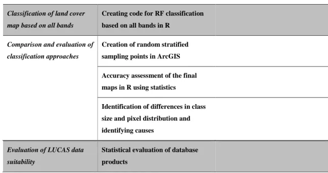
Classification of land cover map based on monthly maps
Creating code for RF classification based on single month maps in R
5 Classification of land cover
map based on all bands
Creating code for RF classification based on all bands in R
Comparison and evaluation of classification approaches
Creation of random stratified sampling points in ArcGIS
Accuracy assessment of the final maps in R using statistics
Identification of differences in class size and pixel distribution and identifying causes
Evaluation of LUCAS data suitability
Statistical evaluation of database products
Table 1 shows the basic objectives in the left column. The related basic processes are displayed in the middle column. The optimisation of the process, if available, is described in the right column. Otherwise it is left blank.
1.3. Outline
The structure of the remainder of the document is as follows: Chapter 2 contains the literature review. It describes the related work previously done in the field, providing background knowledge to this thesis. Chapter 3 presents the data and the study area. Chapter 4 discusses the approach, tools and the methodology that has been used. Chapter 5 presents and discusses results obtained in the thesis. Chapter 6 concludes the project, highlights its contributions and then provides suggestions for further research in the area.
6
2. LITERATURE REVIEW
This Chapter will provide an overview on the literature relevant for the study. The topics covered are land cover classification (multi-spectral and multi-temporal) in Chapter 2.1, Sentinel-2 Multispectral Instrument (MSI) data products in Chapter 2.2, the use of LUCAS data in present literature in Chapter 2.3, the use of Random Forest for land cover classification in Chapter 2.4 and definition and review of the accuracy assessment tools in Chapter 2.5.
2.1. Introduction to Land Cover Classification
A main application in terrestrial remote sensing data is the analysis and classification of land cover. Land cover is always dependent on the study area and includes different classes, such as water, urban areas, and different types of forests and crops. It is a basic variable with high significance for assessing the environment (Foody, 2002). Therefore, accurate and relevant information on land cover are increasingly in demand in many areas of government, economy and science (Homer et al., 2007). Due to the range of applications, thematic maps are thus needed in a variety of temporal and spatial resolutions. Applications include change detection (Singh, 1989), habitat mapping (Schuster et al., 2015; Stow et al., 2008), agriculture (Blaschke, 2010; Deren et al., 2003; Lu et al., 2013), disaster risk management (van der Sande et al., 2003), and vegetation mapping (Karlson et al., 2015; Vaglio Laurin et al., 2016).
Multi-temporal classification is one approach for land cover classification (LCC). It is based on using imagery acquired over a specific time period ranging from several weeks to multiple years for classification. With the steady increase in spatial, spectral and temporal resolution, these classifications now include a multitude of bands on a high spatial resolution of a few meters. This leads to a high dimensionality of data and new challenges in the field.
Pelletier et al. (2016) (which will also be discussed in Chapter 2.4) successfully used Random Forest as a classifier on multi-temporal, multi-spectral satellite imagery. The study is using different tiles of Landsat-8 and SPOT-4 images
7 to simulate S2 data with an average temporal resolution of 13 days from April 2013 until November 2013. An overall accuracy of over 80% was documented. The study concludes that the classifier is able to identify both static land cover types, such as forestry, and dynamic land cover types, such as agriculture.
The study states that RF was able to sufficiently discriminate land cover types by exploiting the temporal information of the spectral signatures alone, though a slight increase in the classification accuracy of dynamic land cover types is indicated. The reportedly small increase in accuracy when using ancillary data is outweighed with a significantly increased computational time.
Yin et al. (2014) ran a similar study of mapping annual land use and land cover changes using a MODIS time series. This particular study also uses RF as the classifier on a pixel-based approach. Based on MODIS VI data, a 16-day product of 250m spatial resolution, they used all available imagery between mid-February of 2000 and December 2001 of a region in Inner Mongolia. The nomenclature used for this study was very similar to the one used in this study, consisting of six land use and land cover classes. These include cropland, forest, grassland, constructed area, water, and bare lands. The study achieved an overall mapping accuracy of 92%. The main uncertainties stated were the confusion between very low vegetated grassland and permanent non-vegetated areas and the confusion between croplands and grasslands. The first uncertainty is explained by the high temporal variance of rainfall and similarities in spectral values. The second uncertainty is caused by similar spectral and temporal patterns of the land cover classes, which makes it difficult to differentiate them solely based on remote sensing data. To achieve high accuracy, the study used both homogenous and heterogenous testing samples to suggest mixed-land cover. The study is concluded highlighting the potential of trajectory-based methods for LULC mapping, specifically to detect land use changes.
Multi-temporal, multi-spectral imagery is also used by Schneider (2012). The study used a variety of machine learning algorithms, one being RF, on 35 to 50 Landsat scenes and NDVI as input bands for three study areas in China for urban change detection. Though achieving good results of 74.6% to 89.4% overall accuracy with RF, the study points out the importance of seasonal information since classes such as bareland, uncultivated or fallow agriculture and new construction sites can
8 easily be confused by the classifier. Other limitations discussed are the computational effort needed to process these large quantities of data and the availability of cloud-free data.
A topic repeatedly discussed for multitemporal studies is the question how single or multiple data acquisition dates affect the classification accuracy (Schmidt et al., 2014; Schuster et al., 2015). Esch et al., 2014 successfully attempted in his study to reduce the effect of specific weather and soil conditions by approximating a general class description for agricultural crops using multi-temporal satellite data. Also Nitze et al. (2015) recognised the positive effect multi-temporal classification can have on classification accuracies.
In conclusion, multi-spectral and multi-temporal data as input for land cover classifications showed high potential, yet are subject to a variety of limitations. These range from financial to the need of large amounts of imagery taken under good atmospheric conditions. The need of remotely sensed time series imagery to cover large areas at high spatial and temporal resolution without becoming too costly was difficult to meet in many studies discussed (e.g. Wardlow and Egbert, 2008). A common trade-off in remote sensing studies is to either chose high spatial or high temporal resolution data (Lambin and Linderman, 2006). Nevertheless, the use of multi-temporal satellite data, especially to classify vegetation, has increased with the improvement of spatial and temporal resolutions of satellite capabilities (Atzberger and Eilers, 2011; Justice and Hiernaux, 1986; Zhang et al., 2003). A recent development in this field was the shift from using relatively spatial coarse data products (250 m to 1 km) from optical sensors such as, TERRA MODIS, ENVISAT MERIS or SPOT VEGETATION (Atzberger and Eilers, 2011; Gu et al., 2010; Jia et al., 2014; Lu et al., 2013; Neves et al., 2015; Nitze et al., 2015; Zhang et al., 2003) to using data products obtained by multi-sensor satellite systems such as RapidEye or Sentinel-2A/B, who provide data products of strongly increased resolutions (Schuster et al., 2015).
9
2.2. Sentinel-2 Data in Present Literature
Not only the technology to acquire the data and its resolutions have been steadily improving, but also its availability. Institutions such as the European Union have committed to an open-access agenda to make data freely available to the public. This development is part of the Big Free Data movement in remote sensing. Sentinel-1A/B as part of the European Copernicus program and Landsat-8 as part of the Landsat project were especially contributing to create freely available data on a regular basis (Kussul et al., 2017).
Two of the most recent additions to sensors creating freely available Earth Observation (EO) data in high resolution were the launches of Sentinel-2A in June 2015 and Sentinel-2B in March 2017 (ESA, 2017a). The twin satellites will share the orbit 180° apart from each other, thus increasing the temporal resolution of products available. With both satellites orbiting, the temporal resolution reached five days (Wang et al., 2016). The Sentinel-2 satellite imagery has been made freely available by the European Commission’s Copernicus program to further research and monitoring. The Multispectral Instrument (MSI) with a swath width of 290 km produces high-resolution imagery with 13 spectral bands (443 nm–2190 nm) available every five days. The spatial resolutions available are 10m (4 visible and near-infrared bands), 20m (6 red-edge/shortwave-infrared bands) and 60m (3 atmospheric correction bands) (Drusch et al., 2012).
Three types of data products are offered on the homepage of the European Space Agency (ESA), which is hosting the Sentinel-2 data: Level-1B products which consist of sensor geometry of top-of-atmosphere radiances. Level-1C products which consist of top-of-atmosphere (TOA) reflectances in a combined UTM projection and WGS84 ellipsoid. And lastly Level-2A products which are bottom-of-atmosphere (BOA) reflectances in a cartographic geometry (ESA, 2017). The product used for this thesis are Level-2AC and Level-1C data products. The latter needs to be processed and formatted to L2A with Sen2Cor (ESA, 2017c; ESA, 2017d), a processor correcting atmospheric effects to produce L2A surface reflectance data (Louis et al., 2016).
All studies based on Sentinel-2 are fairly new since the satellite has only been in orbit since 2015. Therefore, many studies available are based on simulated MSI data to assess the potential of S2 data. Applications range from geological mapping to
10 water body modelling (Clark, 2017; Dong et al., 2015; Drusch et al., 2012; Malenovský et al., 2012; Ramoelo et al., 2015; Van der Meer et al., 2014). For example, Clevers and Gitelson (2013) positively assessed the usability of the red-edge bands of Sentinel-2 as the basis for calculating vegetation. All studies concluded to see high potential in the data derived from the sensor due to its high spatial and temporal resolution.
The selection of scientific papers using actual S2 MSI data in their studies is relatively limited. Fernández-Manso et al. (2016) successfully used S2 data for burn severity, calling the data adequate for this type of study. Classification exercises to map crop types and tree species with Sentinel-2 data by Immitzer et al. (2016) supported this outcome. Other applications include mapping water bodies (Du et al., 2016), monitoring fine-scale habitats (Stratoulias et al., 2015), discriminating forest types (Vaglio Laurin et al., 2016), and forest fire evaluation (Navarro et al., 2017). All studies see high potential in S2 MSI data.
On the subject of whether S2 data differs in usability from other high-resolution sensor products such as Landsat 8, results of studies differ. In a study of 2016, Novelli et al. conducted a performance evaluation test comparing S2 data and Landsat 8 Operational Land Imager data based on their ability to perform object-based greenhouse detection. Both Kappa Index of Agreement and Overall Accuracy of the study indicated that S2 predictions performed consistently better than the corresponding Landsat 8 predictions. This result was attributed to the better performance of S2 features in the RF classification training process. It was concluded that these results indicate S2 as the more stable data source to efficiently extract greenhouses irrespective of atmospheric conditions. On the other hand, Korhonen et al. (2017) found no systematic differences between Landsat 8 and Sentinel-2 in their study on estimating boreal forest canopy cover and leaf area index.
In conclusion, Sentinel-2 data provides high usability for a multitude of applications in the remote sensing field by providing data products of global coverage, fine spatial resolution and relatively fine temporal resolution (Wang et al., 2016).
11
2.3. LUCAS Data in Present Literature
The data used as ground truth was extracted from LUCAS micro-data for Portugal, an OA spatial database1. LUCAS is a geographical in-situ survey conducted every three years since 2000 by the Statistical Office of the European Commission (EUROSTAT) to detect land cover and land use (LULC) changes in the European Union-28 territory (EC, 2017). The point database consists of detailed land cover and land use attributes for large parts of Europe accompanied by respective ground truth photographs (Karydas et al., 2015).
Its primary goal is to provide multi-temporal, comparable statistical information about the participating countries (Karydas et al., 2015). Moreover, it is used to monitor the implementation of the Europe 2020 strategy by providing the data used to calculate agro-environmental indicators, sustainable development indicators and land take. Additionally, it is used for production, verification and validation of land cover mapping initiatives such as Copernicus’ CORINE Land Cover (EUROSTAT, 2016). LUCAS classification is composed of eight main categories indicated by capital letters: A: Artificial land; B: Cropland; C: Woodland; D: Shrubland; E: Grassland; F: Bare land; G: Water areas; H: Wetlands. These main categories are further divided into a total of 76 subclasses. These classes are defined by the combination of the letter of the main class and two to three digits (Karydas et al., 2015).
The sampling process of LUCAS data is conducted in two phases. In the first phase, the territory is covered with a 2x2 km grid to obtain the LUCAS master, containing around 1.100.000 points in Europe. These points are then categorised by photointerpretation of aerial imagery. In the second phase, n out of N points are selected per class and visited in-situ to conduct a more detailed LCLU survey. It is a combined approach of photointerpretation and in-situ information collected during groundwork (EUROSTAT, 2016).
Literature of studies based on LUCAS data are not common. Esch et al. (2014) used LUCAS data for training and evaluation of their classification. The study used an object-based approach to distinguish cropland and grassland in an area of 15km by
1
12 15kmusing multi-spectral, multi-seasonal imagery. It resulted in an overall accuracy (OA) of 86% and a Kappa coefficient of 0.79. A land use land cover mapping approach by Mack et al. (2017) based on the LUCAS points achieved overall high accuracy levels with above 85% for most classes and an overall accuracy of 87%. Nonetheless the study´s suggestions for future work include to concentrate on efficient ways to minimise the quantity of unsuitable LUCAS data for LCC. Both studies also observed imbalanced training data. Other studies using LUCAS data include soil erosion modelling (Panagos et al., 2014), and soil pH mapping (Gardi and Yigini, 2012). It is important to note that all aforementioned studies support their use of the LUCAS database with ancillary data to increase classification accuracy.
Another set of studies used the LUCAS data as reference data for validating large-scale LULC maps based on remotely sensed imagery (Gallego, 2011; Karydas et al., 2015). Karydas et al. (2015) used a comparative approach to determine the suitability of LUCAS data as a reference dataset to validate a Land Cover Map of Greece for 2007. He compared an “automated” classification process entirely relying on the LUCAS main land cover attribute to a “supervised” classification process, where the classification was based on photointerpretation of LUCAS imagery. The automated classification approach resulted in an accuracy of 61.9% while the supervised approach resulted in an accuracy of 51.8%. The study found the database to be supportive yet limited in efficiency to verify the Land Cover Map used in the study. Two of the main issues raised were misclassifications of samples by LUCAS surveyors and that many points were assigned a class from distance and had to be removed from the study. In this particular case, 23.7% of all points used were excluded from assessment. In conclusion, the study suggested that LUCAS could rather be used as a verification than a validation dataset. Similar issues were raised by Gallego (2011), whose study validated then-available EU reference data. This study resulted in 67.3% estimated overall accuracy before increasing the accuracy to 75% by excluding a class from the assessment. Unlike Karydas et al. (2015), this study does not advise against using LUCAS as validation data for land cover maps. Still it states that automatic processing of this data is often insufficient for validation and recommends photointerpretation of the ground truth photography included in the database.
13 Nonetheless, little experience exists in using LUCAS data as the sole input for large-scale LCC. Mack et al. (2017) stated that a specific issue to investigate is the usability of LUCAS data as a training data base for supervised classification approaches, which is one of the two aims of this study.
2.4. The Use of Random Forest for Land Cover Classification
In the last two decades, machine learning algorithms for LCC have been increasingly used and adapted by the scientific community (Lawrence and Moran, 2015). One of the most popular and heaviest tested algorithms is RF, a machine learning ensemble producing a group of decision tree classifiers based on a bootstrapped training set of data (Breiman, 2001; Gislason et al., 2006; Pal, 2005). The most popular and thus final class is identified by having decision tree ensemble vote to achieve the highest accuracy (Breiman, 2001). Nitze et al. (2015) summed the requirements for this classifier up as:
“a reference dataset, containing numerical data (e.g. VI or reflectances) and its corresponding class label for the training of the classifier and its internal accuracy calculation.” (p.5).
This classifier is widely and successfully used to perform classifications and regressions on remotely sensed imagery (e.g. Gislason et al., 2006; Pal, 2005; Stepper et al., 2015). It has been widely and successfully applied for regional land cover mapping using multi-temporal data (Alcantara et al., 2012; Fagan et al., 2015; Rodriguez-Galiano et al., 2012; Zhao et al., 2016) and multi-spectral data (Clark et al., 2012; Gessner et al., 2015; Lawrence and Moran, 2015; Rodriguez-Galiano et al., 2012b; Rodriguez-Galiano et al., 2012a; Zhao et al., 2016).
Advantages for using RF for land cover mapping lay were mentioned in the theoretical framework of the thesis (Chapter 1.1), yet can be summed up as follows: RF as a classifier provides high accuracy and speed in training and application, non-parametric approach to classification, and is able to handle high data dimensionality while being insensitive to overfitting (Belgiu and Dra, 2016). It can be used with categorical, unbalanced, and incomplete data and with little user input while still
14 achieving high classification accuracy, which is not possible with other many classifiers (Clark, 2017; Pal, 2005). As it is relatively insensitive to small sample size relative to its presence in the feature space, also known as Hughes effect, it is suitable for this study. Additionally, RF can be used to detect and rank variables with the highest ability to differentiate between targeted classes. This ability can be very useful and time-saving when working with highly dimensional data such as remotely sensed imagery (Neves et al., 2015). Moreover, by automating the ranking and selection of the most important variables, it makes the selection less subjective and error-prone (Belgiu and Dra, 2016; Belgiu et al., 2014).
A study which incorporates several elements also used in this study is Novelli et al. (2016). The study uses a combination of RF and multi-temporal, multi-spectral S2 data for greenhouse detection sand achieved overall accuracy values ranging from 87.9% to 93.4%.
Pelletier et al. (2016) discusses the use of RF and Support Vector Machines on high spectral, temporal and spatial resolution remotely sensed imagery (Landsat-8 and SPOT-4) as a time-series. The discussion indicates a set of challenges common when using machine learning algorithms for land cover classification: Firstly, to identify the correct classifier to handle the high resolutions and dimensionality of the data. Secondly, to evaluate how stable the classifiers are. Thirdly, how to select the most appropriate feature set for training the classifier while balancing accuracy of the classification and computational time needed. And fourthly, how to maintain classification accuracy over extensive areas. The study concludes with good results for both classifiers, though RF reached a slightly higher overall accuracy. Other studies, where RF provides better results than other classifiers confirm this conclusion (e.g. Schneider, 2012).
Moreover, additional advantages of RF are indicated. These include a small training time and easy parametrisation. Another relevant conclusion of the study is that the setting of parameters has little influence on the classification accuracy. These finding indicate that RF is a suitable algorithm for multi-temporal, multi-spectral classifications of large areas based on spectral bands like in this study.
15
2.5. Accuracy Assessment Tools
Choosing the most suitable accuracy assessment tools is an extensively researched and discussed topic in the field of remote sensing. Not all tools are appropriate for all studies, thus this chapter only discusses the ones applied in this thesis. As stated in the theoretical framework (Chapter 1.1), the accuracy of the results is assessed using reference data bases consisting of samples resulting in kappa coefficient of agreement, confusion matrices and overall, user, and producer accuracy (e.g. Gong et al., 2013; Inglada et al., 2015; Novelli et al., 2016). Additionally, this thesis relies on visual inspection (e.g. Chen et al., 2005; Im et al., 2007; Van der Meer et al., 2014; Li et al., 2016).
An often used tool in land cover classification assessment is an confusion or error matrix. It is describing the pattern of class allocation made by the classifier in relation to a reference data set. One of the measures to be derived from confusion matrices is the percentage of the samples which were correctly allocated, which is indicating the overall accuracy of the prediction. Unlike the kappa coefficient and other measures that can be derived from a statistical assessment of a classification, confusion matrices also make full use of the information content by giving more detailed information on the number of correctly and incorrectly classified samples per class (Congalton and Green, 1993; Congalton, 1991; Foody, 2002). It allows for the accuracy assessment to focus on individual classes. This is enabled by relating the amount of samples which were correctly allocated to the sum of samples in the class. Depending on if the calculations are based on the column or row marginals of the matrix, this results in the so called producer´s and user´s accuracy (Campbell, 1996).
The cross-tabulation of observed ground or reference data to a classified label has established itself as the foundation of accuracy assessment in remote sensing (Canters, 1997). It enables the description of classification accuracy and locate and characterise errors. This information can then be used to refine the classification or correctly assess the results and what they indicate. An example for this is if there is a high rate of confusion between two specific land cover classes in the matrix, ancillary data containing information for the classifier to discriminate the two could increase correct classifications. Moreover, it can help to identify misclassifications in a map
16 and thus give a more accurate idea of the area extent of land cover types. For example, if the confusion matrix helps identifying a class which has a high rate of being misclassified as another class, the extent of the first class seen on a map based on the same classification can be assumed to be higher than depicted (Hay, 1988; Jupp, 1989).
Though using confusion matrices as a tool for accuracy assessment is established and informative, the scope of accuracy assessment should not be limited to this metric (Congalton and Green, 1993). A major problem discussed in the literature is the possibility that the samples were coincidentally assigned to the correct class (Pontius, 2000). Cohen´s kappa coefficient is used as a standard metric to compensate for this effect. It was introduced by the scientific community into studies in a variety of scientific fields. It measures the rate of agreement or disagreement by chance and allows the calculation of a variance term. The significance of the difference between a set of coefficients can thus be calculated (Foody, 2002). A kappa value of 0 indicates an agreement that is equal to complete chance, while a kappa value of 1 indicates complete agreement (Viera and Garrett, 2005). This makes it an attractive metric for assessing classification accuracy.
Nonetheless, e.g. Foody (2002) discusses the kappa coefficient in a critical way. The study is stating that despite its popularity, its ability to compensate for change agreement in classifications and its ability to allow the evaluation of the differences in accuracy is not unique among the accuracy metrics. This disagrees with calls made in literature to establish the kappa coefficient as a standard measure (Smits et al., 1999).
17
3. STUDY AREA AND DATA
This Chapter will introduce the study area (Chapter 3.1) as well as the S2 and LUCAS datasets used (Chapter 3.2.1 and Chapter 3.2.2 respectively) to conduct the research. Moreover, the composition of the nomenclature will be discussed in
Chapter 3.2.2. A detailed description of data processing will be provided in Chapter 4.
.
3.1. Study Area
The selection the study area was conducted by the Direção-Geral do Território (DGT- engl. Directorate-General for the Territorial Development) located in Lisbon, Portugal. One S2 tile of Portugal was chosen as the area of interest. The study region as presented in Figure 1 is a 100km by 100km large area in Central Portugal. Located North-West of Lisbon, it includes the city of Santarém and land East of Santarém along the Tagus river. It was deemed most suitable for the study, since it is covered by a variety of land use and land cover types: According to CORINE Land Cover Map of 2012, the LC types include artificial surfaces (urban fabric, mineral extraction sites, etc.), a variety of types of agricultural areas, forest and semi natural areas, and waterbodies2. Especially because of its agriculture, the cyclic changes in the vegetation over course of a year were expected to be strongly reflected in the reassignment of samples according to their NDVI values. This adds an additional dimension to the analysis.
2 CORINE Interactive Land Cover Map.
18 Figure 1. Study Area in Central Portugal (shapefile taken from DGT, 2017a)
19
3.2. Data
Two different data sets are used in this study: The S2 remotely sensed imagery of the study area and land cover point data extracted from the Eurostat Land Cover/Use Statistics (LUCAS) dataset of 2015 used to build and train the classifier.
3.2.1. Sentinel-2 Imagery
The S2 imagery was obtained free of charge from the Copernicus Open Access Hub3, the online system of the ESA on 21.11.2017. The hub was established to make Sentinel products accessible to data users (Copernicus, 2017).
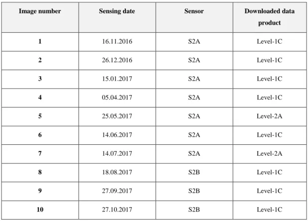
The S2 data products downloaded are 10 sets of 13 bands respectively, each representing the 10 000km2 large site defined in Chapter 3.1. An overview of the data products used is in Table 2. The parameters to identify the appropriate products for the analysis were the following: a sensing period time frame of November 2016 to October 2017 and a cloud coverage percentage of up to 10%. Data could both be derived from S2A and S2B missions. The initial data format is JP2.
3 Copernicus Open Access Hub (2018). Available at: https://scihub.copernicus.eu/dhus/#/home. Last
20 The data products selected are eight Level-1C (L1C) and two Level-2A (L2A) products. L1C data contains top-of-atmosphere reflectance values in a fixed cartographic geometry of combined UTM projection and a WGS84 ellipsoid (Zone 29 North). The L2A data preserves the cartographic geometry, yet contains bottom-of-atmosphere reflectance values (ESA, 2017b).
Unlike data products on lower levels (Level-1A and 1B), these products are radiometrically and geometrically corrected (including orthorectifications and spatial registrations) (ESA, 2017a). To work with the L1C tiles, an additional processing step was required: Through further corrections of atmospheric effects, they were converted to L2A products using the Sen2Cor processor (Louis et al., 2016). The Sen2Cor processor is a tool available in the S2 Toolbox developed for the ESA in the common Sentinel Application Platform (SNAP). It allows analysis, visualisation and processing of MSI data derived from the S2 missions. Processing to Level 2A products calculates bottom-of-atmosphere reflectances in the same cartographic geometry and conducts scene classifications and atmospheric corrections (ESA, 2017c; ESA, 2017d). Details of this process will be provided in Chapter 4.3.
Image number Sensing date Sensor Downloaded data
product 1 16.11.2016 S2A Level-1C 2 26.12.2016 S2A Level-1C 3 15.01.2017 S2A Level-1C 4 05.04.2017 S2A Level-1C 5 25.05.2017 S2A Level-2A 6 14.06.2017 S2A Level-1C 7 14.07.2017 S2A Level-2A 8 18.08.2017 S2B Level-1C 9 27.09.2017 S2B Level-1C 10 27.10.2017 S2B Level-1C
21 The bands used for ground geometry were preselected for the research. Of the 13 bands available through the MSI on Sentinel-2 the following were used: 10m spatial resolution bands B2 (490nm), B3 (560nm), B4 (665nm), and B8 (842nm), and the 20 m spatial resolution bands B5 (705 nm), B6 (740 nm), B7 (783 nm), B8a (865nm), B11 (1610nm), and B12 (2190nm) (ESA, 2017b). The three bands with 60m spatial resolution (B1 (443nm), B9 (940nm), and B10 (137nm)) were each excluded from the analysis. This was done since their data was not useful for this study. Additionally, downscaling them to 10m resolution would drastically decrease the quality of data and output.
The 20m resolution bands were downscaled to 10m using the “raster” package in R (Hijmans et al., 2017). Therefore, the Minimum Mapping Unit (MMU) of this study is a pixel of 10m x 10m.
3.2.2. LUCAS Data and Nomenclature Composition
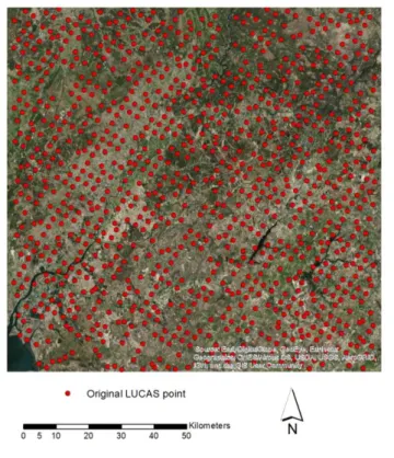
964 LUCAS points were available as ground truth in the study area selected. The records represented 43 sub-categories according to the LUCAS classification which were merged into their eight main land cover categories according to EUROSTAT (2017) (Table 3). The locations of the point features are visible in Figure 2.
LUCAS category
Artificial land
Cropland Woodland Shrublan d Grassland Bare land Water Salt marshes Sample size 50 194 471 79 137 17 14 2
22 The point features were reclassified based on nomenclature used by GeoVille for their HR Land Cover Map for Austria in 2017 (Steidl, 2017) based on a recommendation of Dr. Caetano. The LUCAS technical reference document C3 by Eurostat (EUROSTAT, 2017) was used to correctly reassign every LUCAS sub-class accordingly. The classes composed and their corresponding sample size are visible in Table 4. Definitions of the GeoVille nomenclature class criteria were derived from published material and email contact with Ms. Steidl. In the process, two points of the class “Salt marshes” (H21) were excluded, since the GeoVille nomenclature did not include a comparable class. It was concluded that the removal will not negatively impact the training data. This resulted in a final sample size of 962.
23 Since differentiating permanent from periodic herbaceous is difficult using only spectral values of one month, it was decided to use a binary reclassification scheme for the “Herbaceous periodic” class for the single month maps. Thus, samples of “Herbaceous periodic” were either reassigned to “Non-vegetated unsealed surfaces” or “Herbaceous permanent” (only referred to as “Herbaceous” in single month maps) according to their NDVI value. The threshold for reassignment was set at 0.3, based on recommendations by Dr. Caetano and literature such as Esau et al. (2016). Said paper describes the threshold as significant, stating that surfaces with an NDVI lower than 0.2 normally corresponds to non-vegetated surfaces while green vegetation canopies correspond to an NDVI of >0.3. This process was applied on every single month map to take the Land Cover Change (LCC) caused by seasonal variability into consideration.
From the first experimental classifications with the LUCAS data as training set for the classifier, it became apparent that the data needed to be modified to obtain results with acceptable accuracy. Initial tests on classifying a single month set of imagery achieved an accuracy of 38%. As Table 4 shows, the distribution of samples on classes is unbalanced with sample sizes ranging from 14 to 650 per class. Unbalanced data means an underrepresentation of an important class in the overall data set (Cieslak and Chawla, 2008). In this sample distribution, “Non-vegetated unsealed surfaces” and “Water” can be described as such.
Unbalanced training data is a common occurrence in data science (Cieslak and Chawla, 2008; Jiménez-Valverde and Lobo, 2006), and it is a phenomenon that frequently occurs when studies use LUCAS data (e.g. Karydas et al., 2015; Mack et al., 2017). To increase classification accuracy, the same approach as in Nitze et al. (2015) and Mack et al. (2017) was taken: Additional samples for the classes two and
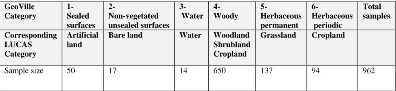
GeoVille Category 1- Sealed surfaces 2- Non-vegetated unsealed surfaces 3- Water 4- Woody 5- Herbaceous permanent 6- Herbaceous periodic Total samples Corresponding LUCAS Category Artificial land
Bare land Water Woodland Shrubland Cropland
Grassland Cropland
Sample size 50 17 14 650 137 94 962
24 three were added to increase information given to the classifier, thus easing the identification of said classes. The approach was to visually identify pure pixels containing a single type of land cover for each class mentioned and label them accordingly. The quantity of added samples was determined by passing the threshold of 50 samples to create more balance and compensate for inaccurate classification attempts during trials. Moreover, initial classification attempts showed the inability of the classifier to distinguish the spectral signatures of water and dense, dark vegetation canopy. Thus 21 samples were added to the class “Woody” to provide additional information. This resulted in a final total sample size of 1056. In addition to this process, some clearly mislabelled sampling points were identified via photointerpretation and moved to reflect their respective class. Not all points were checked. The results of the modifications are in Figure 3.
Table 5 shows the final nomenclature used and how it responds to the input LUCAS nomenclature including its subcategories. The final number of samples can be seen in the right column. Added samples are indicated by their label.
25
ID
Austrian nomenclature
LUCAS main
category LUCAS Sample sub-category No. of samples
1 Sealed surfaces Artificial land A A11 - Buildings with one to three floors
A21 - Non built-up area features A22 - Non built-up linear features
17 13 20 2 Non-vegetated unsealed surfaces Bareland F
F10 - Rocks and stones F20 - Sand
F40 - Other bare soil Additional samples
2 1 14 34
3 Water Water G G11 - Inland fresh water bodies
G21 - Inland fresh running water Additional samples
8 6 39 Excluded Snow and ice Excluded Excluded Excluded 0
4 Woody Woodland Shrubland Cropland C D B C10 - Broadleaved woodland C22 - Pine dominated coniferous woodland
C32 - Pine dominated mixed woodland
C33 - Other mixed woodland D10 - Shrubland with sparse tree cover
D20 - Shrubland without tree cover B71 - Apple fruit
B72 - Pear fruit B73 - Cherry fruit B74 - Nuts trees
B75 - Other fruit trees and berries B76 - Oranges B81 - Olive groves B82 - Vineyards B83 - Nurseries Bx2 - Permanent crops Additional samples 363 80 25 3 53 26 4 3 1 1 5 2 65 15 1 3 21 5 Herbaceous permanent Renamed to "Herbaceous" in single month maps
Grassland E
E10 - Grassland with sparse tree/shrub cover
E20 - Grassland without tree/shrub cover
E30 - Spontaneously re-vegetated surfaces 33 75 29 6 5 or 2 Herbaceous periodic Reclassified into "Herbaceous" or "Non-vegetated unsealed surfaces" depending on NDVI value in single month maps (Threshold: 0.3) Cropland B B11 - Cereals B12 - Durum wheat B15 - Oats B16 - Maize B17 - Rice B18 - Triticale B19 - Other cereals B21 - Potatoes B31 - Sunflower B42 - Tomatoes
B43 - Other fresh vegetables B53 - Other leguminous and mixtures for fodder
B54 - Mixed cereals for fodder B55 - Temporary grasslands Bx1 - Arable land 2 1 5 33 7 1 1 4 1 13 3 2 1 10 10 Excluded Reeds Excluded Excluded Excluded 0 Excluded No match Excluded Excluded H21 - Salt marshes 2
26
4. APPROACH, METHODOLOGY AND TOOLS
This section will give an overview over the approach selected as well as the methodology used. Chapter 4.1 explains the approach taken and gives an overview over the general methodology of the work. It is followed by Chapter 4.2, which gives an overview over all tools used in this study. Chapter 4.3 contains detailed information on the processing of S2 and LUCAS data, followed by the detailed methodology of the analysis conducted in R in Chapter 4.4. Finally, the processing of the modified LUCAS data is described in Chapter 4.5.
4.1. Approach and General Methodology
The general approach to answering the research questions was kept in close co-operation with the DGT and the co-supervisor of this thesis, Dr. Mário Caetano. The mapping approach is raster-based with 10m pixel size as the MMU, using categorical values for the land cover classification. For choosing this approach the characteristics of the satellite data, such as its spatial and temporal resolution, as well as the type of thematic information to be extracted have been considered. The characteristics of the geographical area to be mapped, specifically the existing land cover types, and the availability of ancillary data have also been taken into consideration in the general approach, resulting in the nomenclature introduced in Chapter 3.2.2. Regarding the classification algorithm, a hard (crisp) classification was used. Unlike with soft (fuzzy) classification, each pixel gets assigned a membership in one definite class (De Matteis et al., 2015). RF was selected, since it is a non-parametric classifier it does not require any assumption about the statistical distribution of the training data while providing good computational efficiency and easy understanding of the classification process (Belgiu and Dra, 2016).
The sample selection for the training phase of the classifier was entirely based on the LUCAS data. Thus, the basic sample size was pre-determined. Additional samples were added to balance underrepresented classes in the training data set as discussed in Chapter 3.2.2.
Equalised stratified random points were created in ArcGIS were used as accuracy assessment points of 50 samples per class, following the recommendation of the DGT.
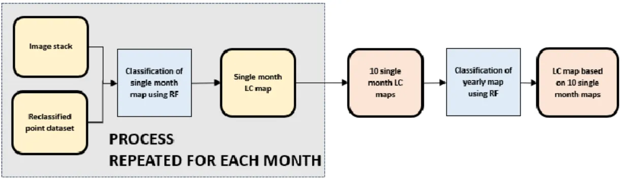
27 The flowchart showing the methodology to conduct the classification comparison is provided in Figure 4. The general flowcharts is composed of the elements listed: unprocessed input data (grey), processes (blue), interstage products (yellow), and final outputs (orange). The grey box indicates the process which had to be repeated ten times, once of each set of single month data.
It consists of six processes necessary to answer the research questions. These sub-processes will be explained in the Chapter 4.3 and following. All tools used for the analysis are detailed in Chapter 4.2.
28 Figure 4. Flowchart showing the methodology of the classification comparison
29
4.2. Tools
This chapter provides an overview of the tools used in this thesis. Table 6 shows the tools and respective versions involved in the processing steps. Due to issues with processing capabilities of the author´s computer, the initial computing of the single month maps and all predictions for answering the second research question were done at the DGT using multicore computing. All codes written are in Appendix C.
Process Tool Version
General processing PC 4-core system
300 Gigabyte disc space Multicore computing PC 8-core system
1,8 Terabyte disc space Processing S2 L1C to L2A
data
SNAP and Sentinel Toolbox 6.0.0 Sen2Cor 2.4.0 Python 2.7.13 Conversion of S2 data from JP2 to TIF GDAL 202 MSVC 2010 Win64
Processing of LUCAS data ArcGIS Desktop 10.5.1
Creation of accuracy assessment points Pixel redistribution analysis Map creation Downscaling of 20m resolution bands R/ RStudio 3.4.2 (64-bit) Value conversion/NDVI calculation Reclassification of
nomenclature Packages caret ggplot2 raster sp lattice rgdal randomForest e1071 lulcc snow Random Forest classifications Accuracy assessment
Creation of graphs Excel 1712 Class change analysis
Table 6. Tools and related processes in overview
6.0-77 2.2.1 2.6-7 1.2-5 7.3-47 1.2-16 4.6-12 1.6-8 1.0.2 0.4-2
30
4.3. Processing of S2 and LUCAS Data
This chapter gives an overview on the processing flows of S2 and LUCAS data used to create the basic interstage products. All future processing is dependent on the execution of those steps.
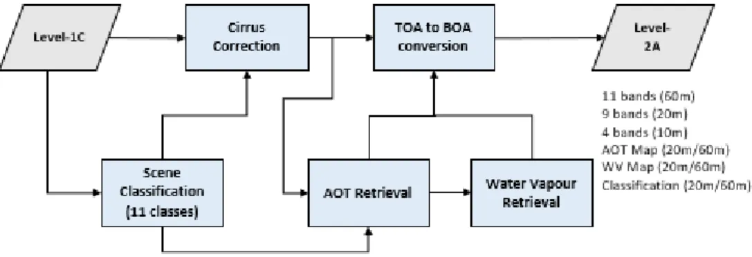
Figure 5 shows the processing steps of the S2 data to create the image stack used with the classifier. All 130 bands are processed using SNAP´s Sen2Cor toolbox. In this process radiance values are converted into reflectance. This step includes the 30 bands of 60m resolution, since they need to be included in the batch for the processor to function. Additionally, the S2 L2A processing creates L2 ortho-image reflectance products (BOA reflectance) from L1C granules in TOA reflectance. The L2A-processing can be divided into two parts: The Scene Classification provides a pixel classification map (cloud, cloud shadows, vegetation, soils/deserts, water, snow, etc.) and the Atmospheric Correction aims at transforming TOA reflectance into BOA reflectance (Figure 6) (ESA, 2017e) .
The processing starts with the Cloud Detection/Cirrus Correction and Scene Classification followed by the retrieval of the Aerosol Optical Thickness (AOT) and the Water Vapour content from the L1C product. The final step is conversion from
Figure 6. Sen2Cor main processing steps (adapted from Louis et al. (2016)) Figure 5. Methodology flowchart of S2 data processing
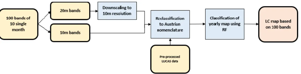
31 TOA to BOA (ESA, 2017e). The L2A products are in JP2 format and need to be converted to GeoTIFF for processing in R (2017). For the conversion of all bands, batch conversion was advisable. Thus GDAL (GISInternals, 2017) USGS Raster Conversion Scripts (USGS, 2017) via Windows Command Prompt was used. Subsequently, the bands are divided into monthly batches. The following processing step is the division of the bands according to their spatial resolution in R. The 30 bands of 60m resolution are removed and the 60 bands of 20m resolution are disaggregated to 10m resolution and joined with the initial 40 bands of 10m resolution to a raster stack consisting of 100 bands. Additionally, the NDVI values are extracted from each 10-band single month dataset as a raster using the following equation:
NDVI= (Band 8-Band 4)/(Band 8+Band 4)
This corresponds with the general formula for calculating the NDVI:
(Matsushita et al.,2007; Schmidt et al., 2014).
The processing of the LUCAS 2015 data is shown in Figure 7. After a data type conversion from CSV to shapefile, the data is processed in ArcGIS. This includes removal of unconfident sample points, data cleaning, cropping and additional
sampling, as explained in Chapter 3.2.2. It is then reclassified in R using the Austrian nomenclature and “Herbaceous periodic” values are reassigned to “Non-vegetated unsealed surfaces” or “Herbaceous permanent” respectively depending on their NDVI value (Chapter 3.2.2).