Does Quantitative Easing have an impact on
European equity markets?
Joana Pereira dos Santos Penida
152415011
Dissertation written under the supervision of Joni Kokkonen
Dissertation submitted in partial fulfilment of requirements for the
MSc in Finance, at the Universidade Católica Portuguesa, April 2017.
Does Quantitative Easing have an impact on European equity
markets?
Joana Pereira dos Santos Penida
ABSTRACT
English
We examine whether the European Quantitative Easing program has an impact on equity markets, considering eight benchmark equity indices and applying a multivariate regression model. During the announcement period of the program, we find evidence of positive abnormal returns in 5 out of 8 benchmark indices, consistent with the portfolio rebalancing
mechanism. When considering the launch period, we find positive abnormal returns in the
German index (DAX30) and negative variations for both Spanish (IBEX35) and French (CAC40) indices. Furthermore, we suggest that the benchmark indices seem to react differently, depending on the country exposures to the program, for both announcement and launch periods.
Português
Examinamos se o programa europeu de Quantitative Easing tem impacto nos mercados de ações, considerando oito índices de referência e aplicando um modelo de regressão multivariada. Durante o período de anúncio do programa, encontramos evidências de retornos anormais positivos em 5 de 8 índices de referência, resultado consistente com o mecanismo de reequilíbrio de portfolio. Quando considerando o período de lançamento, encontramos retornos anormais positivos no índice alemão (DAX30) e variações negativas para os índices espanhol (IBEX35) e francês (CAC40). Além disso, sugerimos que os índices de ações de referência parecem reagir de forma diferente, dependendo da exposição do país ao programa, tanto considerando o período anúncio como o período de lançamento.
Acknowledgements
Writing a master thesis has showed me how hard is to know when and where to stop and start, within so many readable knowledge. We need to have a strong and determined filter to make the right or the most accurate analysis.
First, I would like to thank my supervisor Professor Joni Kokkonen who helped and clarified me every time I had questions. His support and readiness were key elements to overcome my doubts and explore new matters. At the beginning, I thought it could be not possible to approach such a recent topic in the markets but then we found the way to get the method.
I also thank Católica Lisbon School of Business and Economics as an institution of excellence. Likewise, I acknowledge Fundação para a Ciência e a Tecnologia (FCT) for financial support.
Furthermore, I think this work could not be done without all conversations and discussions with Martim. His love and patience made me realize how important is to close a chapter in our lives with constant effort and resilience. I would also thank my family to their presence and comfort.
Contents List
Acknowledgements ... ii
1 Introduction ... 1
2 Quantitative Easing in the European Union ... 5
3 Methodology ... 7
3.1. Event Study: Multivariate and Seemingly Unrelated Regression Models ... 7
4 Data ... 10
4.1. Descriptive statistics ... 10
5 Main Results ... 13
5.1. PSPPa – Quantitative Easing program announcement ... 13
5.2. PSPP1 – Quantitative Easing program launch ... 14
5.3. All dummies - Average ... 16
5.4. Time-varying dummies ... 18
5.5. Excluding the market portfolio ... 20
6 Further Research ... 24
7 Conclusions ... 25
8 References ... 27
1 Introduction
Monetary policy is characterized by the control of money supply in the economy, where price stability is reached through changes in key interest rates. According to Keynes (1936), interest rates are the equilibrating factor between liquidity and its demand, which is directly affected by investors’ liquidity preference. Moreover, adjustments in interest rates occur as a result of changes in inflation target levels (Taylor, 1999).
At the end of the 80s, conventional monetary policy is empirically analyzed and studies from Clarida et al. (1999) point out that the policy is effective in influencing the short-term path of the real economy. Over expansionary times, central banks have a conventional intervening role in managing the liquidity conditions in the market and price stability by controlling the interest rates’ levels and regulating the target inflation. The most common use of such role is to lower interest rates to levels close to the zero lower bound, creating an environment of increasing levels of both individuals’ consumption and firms’ investment.
However, when an economy is already under zero interest rates, one might question whether the policy is producing effective results for the economy. Hereupon, unconventional monetary policies emerge under the zero lower bound (ZLB) environments as a solution to re-establish economic relations (including financial intermediation) and to push the economy towards sustainable growth. Usually, this policy follows a mechanism of large expansion of banks’ reserves through asset purchases programs, inducing potential changes in long-term key interest rates rather than only in short-term official rates (Joyce et al., 2012).
The most well-known case of unconventional monetary policy is Japan’s economy in the end of the 90s. Under a deflationary environment combined with the Zero Lower Bound (ZLB), the Japanese conventional monetary policy lacks in terms of its means to stimulate aggregate demand, where the expansion of liquidity levels does not increase the investors’ willingness to spend extra cash. This phenomenon is known as liquidity trap (Krugman, 1998). To settle this flaw, in March 2001 the Bank of Japan introduced its Quantitative Easing program where the high level of central cash reserves held by the banks would be more than sufficient to spread across the economy (Joyce et al., 2012), yet the huge Japanese national debt and persistent levels of zero inflation made it difficult.
According to Schenkelberg and Watzka (2013), although there is a decrease in the Japanese long-term interest rates and an increase in price levels, those effects are transitory and only supported the economy and inflation growth for a short-term period. Moreover, factors such as exchange rates and US stock prices also influenced Japanese stock prices (Kurihara, 2006).
From the beginning of the financial crisis in 2007-2008, other central banks have been conducting similar unconventional monetary policies. In the United States, one of the largest responses by the Federal Reserve (FED) is the Troubled Asset Relief Program (TARP). Intended to support the banking and the financial system as a whole, the program includes large purchases of non-performing assets from financial institutions. Empirical evidence suggest that the program has been helpful in mitigating the credit risk associated with the financial turmoil, however Black and Hazelwood (2012) indicate that, for large TARP recipients, the average risk-taking increased more than for non-TARP recipients. Furthermore, Harris et al. (2013) state that banks’ efficiency decreased for TARP banks since asset managers of TARP receipts may default in terms of achieving the desired asset management quality.
Between the end of 2008 and October 2014, the Federal Reserve decided to extend its interventions and implements the Large-Scale Asset Purchase Program (LSAP) to enhance the economic activity and further stimulate job creation. According to Gagnon et al. (2010), the program is successful in stimulating the US economy mainly by lowering both the 10-year term premium and long-term private borrowing rates. However, the program has little marginal effect on inflation levels and GDP growth evidence is tiny (Chen et al., 2011).
Following the collapse in the US markets, the Bank of England approached its monetary policy and adopted the same unconventional policy applied at that time. According to Joyce et al. (2012), both the United States and the Bank of England’s Quantitative Easing programs are projected to create shocks in the yields / prices rather than merely solve banking liquidity issues. In detail, the first round of the UK’s Quantitative Easing program (March 2009 to February 2010) is effective in reducing conventional gilt yields by 100 basis points (Joyce et al., 2011). Moreover, FTSE All-Share index and other international equity indices register a decrease in their respective prices around the announcement of the UK’s QE program, suggesting a slightly negative effect on equity markets.
Observing these complex changes in developed economies, it may be relevant to understand if the adopted monetary policies based on money supply are truly effective to reach its economic goal and which factors influence potential losses of effectiveness. This fact may bring the discussion whether there is demand for market liquidity by consumers and investors or, instead, they have decreased their levels of risk tolerance. The persistent world crisis that perpetuates and the zero lower bound (ZLB) environment, combined with weak projected long-term economic growth, made Krugman (2013) refresh Alvin Hansen’s idea where the world is presented as being under a secular stagnation, in which the pattern is characterized by insufficient investment demand and low consumption regarding new sources of capital. Likewise, Summers (2015) supports and claims that the risk of moving towards a secular
stagnation is greater for the Eurozone and Japan’s economies rather than for the United
States.
In this study, we analyze the impact of the European Quantitative Easing on equity markets since there is a lack of literature in analyzing the effects of the program in this specific asset class. For implementation, the study is conducted for eight European benchmark equity indices where we apply a Multivariate Regression Model (MVRM), proposed by Binder (1985) and jointly estimate the regression coefficients under the context of the Seemingly Unrelated Regression Model (SURM), presented by Zellner (1962). The intuition behind this estimation lays on the possibility of having event clustering in the analysis, potentially inducing contemporaneous covariance between the equity indices’ residuals (Section 3.1.). We choose an event window of (-5,5) days to sufficiently cover the effects around the Quantitative Easing program announcement and launch.
Our results show that in the days around the program announcement, the European equity markets seem to react positively although in some cases (Spain, Austria and Portugal) the announcement evidences negative abnormal reaction for the benchmark equity indices. The political instability and the uncertainty associated with changes in governments may be factors that better explain this effect. For the days around the launch, we obtain negative variations in most of the indices, except for Germany. Here, it may be plausible to claim that the existing correlation between German economic system and the purchases from the ECB is crucial to influence asset prices to go up. This positive change may be also consistent with the mechanism of portfolio rebalancing (Tobin, 1969), evidencing a positive perception from investors to allocate their wealth into riskier assets as it is the case of equity classes.
Additionally, when excluding the market portfolio as an explanatory variable, we identify a positive pattern of abnormal equity returns in reaction to the Quantitative Easing announcement, especially for the three countries with the highest value of cumulative monthly net purchases from ECB (Germany, France and Italy). Therefore, one might point the exposure of different equity markets to the program as an explanatory factor for these abnormal variations in returns. During the days of the program launch, it seems that the program causes positive abnormal changes in returns (except for Spain) yet it lacks statistical significance.
This study is organized as follows: Section 2 presents an overview regarding the effectiveness of Quantitative Easing, proposed by ECB, and which mechanisms the program may induce. Section 3 describes the applied methodology for this study and Section 4 presents the chosen sample data. Section 5 outlines the main results obtained following the methodology; likewise, it presents some explanations for them. Section 6 presents a suggestion regarding further research on this topic. Lastly, Section 7 exposes a reflection and main conclusion remarks that include both results and arguments that support all research.
2 Quantitative Easing in the European Union
After establishing the Economic and Monetary Union in the end of 90s, the European Central Bank (ECB) defined a monetary policy focused on maintaining price stability by setting the inflation rate close and up to 2 percent. For that purpose, it uses conventional policy instruments to achieve the main economic goal, by simply managing key interest rates.
Nevertheless, in response to the financial crisis of 2007-2008, the ECB changed its monetary policy approach since it faced a downward environment trapped by large public and private debts. With interest rates below one percent, the European Union introduced its initial program of asset purchases in May 2010 where the central bank began its Securities Markets Program (SMP) to steady the economic transmission mechanism. Two years later, the program is substituted by the Outright Monetary Transaction (OMT).
In literature, Gambacorta et al. (2014) analyze the macroeconomic effects of asset purchases policies and, by using a panel vector autoregression (VAR) for eight advanced economies including the Euro area, find that an injection of liquidity on central banks’ balance sheets creates a transitory positive effect in the economic output and an increase in asset prices. However, the continuous decline in the Eurozone inflation rate combined with low interest rates leads us to consider that the programs fell short on expectations.
Under the persistent goal of achieving price stability and generating extra stimulus in the economy under the Zero Lower Bound (ZLB) environment, on January 22, 2015 the ECB announced the Public Sector Purchase Program (PSPP), known as Quantitative Easing (QE), characterized by massive purchases of long-term assets. In detail, it incorporates Eurozone national government bonds and other assets from the private sector.
From the program launch on March 9, 2015, there is already plenty of research discussing how effective the European Quantitative Easing program may be in supporting the economy in the long-term as well as in achieving the target inflation rate. For instance, Demertzis and Wolff (2016) point out that the effects of the European Quantitative Easing program are too premature to identify and it is hard to understand which are the most affected asset classes relative to the program’s magnitude. Nevertheless, Andrade et al. (2016) find a positive general progression in the European economy, with higher prices in all sectors, subsequently of the PSPP announcement. Likewise, Bernanke and Kuttner (2004) claim that a decrease in
target interest rates leads to an increase in stock price indices. Additionally, Claeys and Darvas (2015) discuss that stock prices should increase due to the portfolio rebalancing
channel. One might suggest that, if the long-term interest rates move towards zero as a
reaction of large purchases of long-term assets, investors may be influenced to rebalance their portfolios by allocating their wealth from bonds to riskier asset classes, as it is the case of the stock market.
This mechanism is initially approached by Tobin (1969) and assumes that money may not be a perfect substitute for government bonds (assumption of imperfect substitutability). Indeed, whether this hypothesis applies, equities and corporate bonds seem to be the closest substitutes for the purchased assets (Joyce et al., 2011) because the portfolio shift from investors intends to increase rates of return and, therefore, improve portfolio’s performance. Considering that this adjustment occurs on risky assets demand, one might state that it causes an upward movement in prices as well as a risk-return trade-off for investors, since the increasing levels of risk enhances portfolio returns. Further, the portfolio rebalancing channel is pointed out by Joyce et al. (2011) and Demertzis and Wolff (2016) as the first response mechanism from investors in reaction to unconventional monetary policies of asset purchases.
On the other hand, the current economic situation is unconventional and the economic relations may not hold. For instance, the mechanism of portfolio rebalancing may not be adequate to reflect investor’s decisions. A research from Assefa et al. (2016) shows the presence of negative effects of interest rates on stock market indices returns of developed countries (characterized by falling interest rates). Those effects may be a result from the lack of effectiveness from the unconventional monetary policy under the Zero Lower Bound environment (ZLB). Whether we consider the weak economic recoveries over time, one might suggest that investors would have less risk tolerance levels and distrust regarding the European financial system as well as related monetary policies (Delivorias, 2015). Furthermore, one might also identify the existing political and unstable economic environments in the Eurozone countries as explanatory factors for the negative reactions from equity markets to the Quantitative Easing program.
3 Methodology
According to MacKinlay (1997), an event study can be defined as the methodology to evaluate whether there is an abnormal change in returns caused by an impact from a certain economic or political event on a set of financial variables. The methodology aims to verify whether the returns are statistically normal or abnormal, in comparison with their realized returns. Thus, this study tries to understand whether there is a short-term impact of the European Quantitative Easing program on financial markets, across a set of Eurozone countries by considering the benchmark equity index for each country.
3.1. Event Study: Multivariate and Seemingly Unrelated Regression Models
In this study, the event windows overlap across equity indices meaning that the calendar days of the event are common to all. This may be a constraint for the standard application of the event study methodology. When event clustering occurs, one might state the presence of correlation between the standard error estimates (Pynnönen, 2005), heteroscedasticity and contemporaneous covariance between country-based residuals (Henderson, 1990).
To handle and overcome these statistical issues, we employ a Multivariate Regression Model (MVRM), proposed by Binder (1985), that incorporates dummy variables for the days into the event window, accounting for the existence of an certain event. Conceptually, M equations are jointly estimated under the context of a Seemingly Unrelated Regression Model (Zellner, 1962), which takes into account residual terms’ correlations among equations. Similar approaches have been applied by a considerable number of authors as it is the case of Collins and Dent (1984), Thompson (1985) and, recently, by Kim, Nam and Wynne (2009).
The multivariate regression is estimated by using a (-5,5) event window and it incorporates dummy variables 𝐷𝑖𝑡 for each day in the event window, including the event day. Here, the regression coefficients represent the abnormal returns of the financial variables. The multivariate regression model is structured as the following:
𝑅𝑖,𝑡 = 𝛼𝑖 + 𝛽𝑖𝑅𝑚,𝑡 + ∑ 𝛾𝑖,𝑎𝐷𝑎,𝑡+ 𝜀𝑖,𝑡 (1)
where 𝑅𝑖,𝑡 is the log return of the index i during the day t, 𝛼𝑖 is the intercept for index i, 𝛽𝑖 is the slope coefficient on the market portfolio and 𝑅𝑚,𝑡 is the log return of the market portfolio.
Then, 𝛾𝑖,𝑎 is the slope coefficient on the dummy variable, 𝐷𝑎,𝑡, that represents either the Quantitative Easing announcement (PSPPa) or launch (PSPP1) if 𝐷𝑎,𝑡 = 1 in all days in the event window and zero otherwise. 𝜀𝑖,𝑡 is the error term (residual), representing the remaining factors that may affect the returns of each index i during the days t, apart from the studied unconventional monetary policy.
All M multivariate equations are jointly estimated by using a two-step estimator of the Seemingly Unrelated Regression Model (SURM), where each regression estimator is first estimated by an OLS regression and then optimized to obtain a FGLS estimator. Approached by the theory, under the presence of heteroscedasticity, a FGLS estimator incorporated in a suitable model (as it is SURM, for instance) is more effective than the single OLS estimator.
In application, we conduct the model in four different forms. First, we include an event dummy 𝐷𝑎,𝑡 in the multivariate regression (1). For each time-series equation we regress the dependent variable (index i) on both market portfolio 𝑅𝑚,𝑡 and on the dummy variable 𝐷𝑎,𝑡. The regression does not include two dummies (PSPPa and PSPP1) simultaneously.
𝑅𝑖,𝑡 = 𝛼𝑖 + 𝛽𝑖𝑅𝑚,𝑡+ 𝛾̅𝑖,𝑎𝐷𝑎,𝑡+ 𝜀𝑖,𝑡 (2)
Second, we consider a single dummy 𝐷𝑎,𝑡 = 1 in all days of the existing event windows, each time we consider an event related to the European Quantitative Easing. Applying the multivariate regression (2), it only shifts the interpretation of 𝛾𝑖,𝑎 in (1) from individual abnormal returns to average abnormal returns 𝛾̅𝑖,𝑎 of index i. While the first methodology is used to access the individual impact of each event (either PSPPa or PSPP1), the second approach shows its average impact in a certain index.
Third, we incorporate time-varying dummies in the multivariate regression (1), as referred by Pynnönen (2005) and recently followed by Rivolta (2014). Here, for each day in the event window, we apply a dummy variable 𝐷𝑎,𝑡 equal to 1, allowing the analysis of existing variations of index returns in each day and pointing out which day represents the highest change, inducing the presence of abnormal returns.
There are only 10 time-varying dummies as consequence of excluding the T-5 dummy, avoiding potential problems associated with the correlation between two or more predictors
(i.e. dummies)1. The model is jointly estimated for both PSPPa and PSPP1 (announcement and launch, respectively).
In the last application of the model, we exclude the market portfolio (EUROSTOXX) from the multivariate regression (1) to isolate the impact of the program on equity indices and to verify which abnormal variations occur in returns by considering a single explanatory variable: The Quantitative Easing dummy (either PSPPa - announcement or PSPP1 - launch). We also do the process for the average abnormal return approach, by using the average dummy variable 𝛾̅. For this last process, we only consider the full sample period.
To verify the appropriateness of the model, which takes into consideration potential correlations among country residuals as well as non-constant variance, we present the Breusch-Pagan test of independence (3), a 𝜒2statistic with 𝑀 (𝑀−1)
2 degrees of freedom, for all processes where we apply the Seemingly Unrelated Regression model. The test (𝜆) is estimated as the following:
𝜆 = 𝑇 ∑ ∑ 𝑟𝑚𝑛2 𝑚−1 𝑛=1 𝑀 𝑚=1 (3)
where 𝑟𝑚𝑛 represents the correlation between the errors of the M equations and T the number of sample observations. Here, the null hypothesis is the presence of homoscedasticity, i.e., constant variance. If the null hypothesis is rejected, we may state the statistical evidence of heteroscedasticity.
1
4 Data
Our sample comprises of daily log returns of eight European benchmark equity indices from Eurozone countries, where each index is used to represent a particular country involved in the European Quantitative Easing program.
We include the following equity country indices: DAX30 index for Germany, CAC40 index for France, MIB is the FTSE MIB for Italy, AEX index for the Netherlands, IBEX35 index for Spain, ATX index for Austria, BEL20 index for Belgium and PSI20 index for Portugal. These countries are chosen based on the amount of cumulative monthly net purchases, as at 31st October 2016, available on ECB website2, following the criteria “greater or equal than 20 trillion of euros” (See Table 9 in the Appendix). Additionally, in the multivariate regression, we include market portfolio as an explanatory variable. We consider EUROSTOXX index, which is a liquid subset of the STOXX EUROPE 600 index that represents large to small capitalization companies of eleven Eurozone countries: Austria, Belgium, Finland, France, Germany, Ireland, Italy, Luxembourg, the Netherlands, Portugal and Spain. All data for the study is extracted from Thomson Reuters DataStream.
We include full sample observations from January 2, 2012 to October 31, 2016 to cover both announcement (PSPPa) and launch of ECB Quantitative Easing (PSPP1): January 22, 2015 and March 9, 2015, respectively. We do not include data before 2012 to exclude the periods of financial crisis, since it is an event with significant impact on the European economy and its financial markets. Also, we consider a subsample period with observations ranging from January 2, 2014 to December 31, 2015 to access comparing or distinct results that may occur during the 5-year sample period, due to the existence of other potential relevant financial or economic events.
4.1. Descriptive statistics
This subsection presents essential descriptive statistics for each European benchmark equity index, to evidence the key differences across Eurozone countries. In Table 1, the descriptive statistics are Mean and Standard Deviation. Moreover, in this subsection, Table 2 presents the correlation coefficients between the eight European benchmark equity markets.
Panel A of Table 1 presents the summary statistics for the full sample period from January 2, 2012 to October 31, 2016. According to the panel, most of the chosen European benchmark equity indices register, on average, positive returns except the Portuguese market index (PSI20). Panel B presents the summary statistics for the subsample period from January 2, 2014 to December 31, 2015. On average, some negative returns emerge for certain benchmark equity indices, as it is the case of IBEX35 and ATX, while the remaining European benchmark equity indices hold their positive mark.
Table 1 – Summary Statistics. This table presents the summary statistics for the eight European benchmark
equity indices plus the market portfolio. The benchmark equity indices are the following: DAX30 is the German index, CAC40 is the French index, MIB is the FTSE MIB for Italy, AEX is the Dutch index, IBEX35 is the Spanish index, ATX is the Austrian index, BEL20 is the Belgium index and PSI20 is the Portuguese index. EUROSTOXX is the proxy for market portfolio. Panel A presents the summary statistics for the full sample period from January 2, 2012 to October 31, 2016. Panel B presents the summary statistics for the subsample period from January 2, 2014 to December 31, 2015. Here, both mean and standard deviation (Std Deviation) are presented in percentage and annualized from daily log returns of each index (one average, each year includes 250 daily observations).
Panel A: Full Sample Panel B: Subsample
Mean (%) Std Deviation (%) Mean (%) Std Deviation (%)
Germany (DAX30) 11.89 19.25 4.99 20.33 France (CAC40) 7.40 19.59 4.22 19.54 Italy (MIB) 2.57 25.82 5.99 23.98 Netherlands (AEX) 7.62 17.01 4.93 17.97 Spain (IBEX35) 1.43 23.01 -1.62 20.14 Austria (ATX) 5.55 19.42 -2.99 18.37 Belgium (BEL20) 10.96 16.43 12.09 15.96 Portugal (PSI20) -3.20 20.84 -9.96 22.57 Eurozone (EUROSTOXX) 7.72 18.59 4.84 18.71
Panel A of Table 2 reports the correlation coefficients between the chosen eight European benchmark equity indices, for the full sample period from January 2, 2012 to October 31, 2016. In this range of observations, all correlation coefficients are positive and greater or equal 0.70. According to Knif et al. (2007), high correlation coefficients may be explained by the presence of volatility in both internal and external markets. Moreover, the increasing level of market integration may also cause the increasing correlation among national stock markets. Further, Hyde et al. (2007) recall that market integration tends to influence stock returns correlations, especially when under bear market periods.
Table 2 – Correlation coefficients. This table presents the correlation coefficients between the eight chosen European benchmark equity indices, for the full sample period
ranging from January 2, 2012 to October 31, 2016. The eight country benchmark equity indices are the following: DAX30 is the German index, CAC40 is the French index, MIB is the FTSE MIB Italy, AEX is the Dutch index, IBEX35 is the Spanish index, ATX is the Austrian index, BEL20 is the Belgium index and PSI20 is the Portuguese index. All results are followed by their statistical significance levels: 10%, 5% and 1%, represented by *, ** and *** respectively.
Panel A: Full Sample
Germany (DAX30) France (CAC40) Italy (MIB) Netherlands (AEX) Spain (IBEX35) Austria (ATX) Belgium (BEL20) Portugal (PSI20)
Germany (DAX30) 1.00 0.93*** 0.82*** 0.91*** 0.79*** 0.78*** 0.89*** 0.70*** France (CAC40) 1.00 0.87*** 0.93*** 0.86*** 0.80*** 0.92*** 0.74*** Italy (MIB) 1.00 0.82*** 0.89*** 0.78*** 0.84*** 0.74*** Netherlands (AEX) 1.00 0.80*** 0.78*** 0.91*** 0.72*** Spain (IBEX35) 1.00 0.77*** 0.83*** 0.74*** Austria (ATX) 1.00 0.80*** 0.69*** Belgium (BEL20) 1.00 0.73*** Portugal (PSI20) 1.00
5 Main Results
In this section, we present all relevant results obtained by following the four different methodologies described in Section 3. In detail, we analyze the abnormal variations in equity returns caused by both European Quantitative Easing program announcement and launch.
In the following subsections, the multivariate regressions coefficients for both full sample (from January 2, 2012 to October 31, 2016) and subsample periods (from January 2, 2014 to December 31, 2015) are reported based on each dummy or dummies: PSPPa – Quantitative Easing program announcement; PSPP1 – Quantitative Easing program launch; All dummies – Average; Time-varying dummies; Excluding the market portfolio. For consistence, each of the following subsections results presents the Breusch-Pagan test of independence (3), obtained by considering each residuals’ correlation matrix.
5.1. PSPPa – Quantitative Easing program announcement
Panel A of Table 3 presents the coefficients of the multivariate regression (1) for the full sample period from January 2, 2012 to October 31, 2016. The multivariate regression includes eight equations, one for each European benchmark equity index, and considers two independent variables: the EUROSTOXX, a proxy for the market portfolio, and the dummy PSPPa accounting for the program announcement. Although most of the obtained coefficients for the PSPPa dummy are positive, they lack statistical significance.
On the other hand, the announcement impact on the ATX index seems to be negative, statistically significant at 10% level. Here, one might suggest that the Austrian investors may not adjust their portfolio allocations during the announcement period, hence not pushing equity prices up. Indeed, at the days that followed the announcement of the program, the Austrian index (ATX) register, one average, more negative returns in comparison with the remaining equity indices (See Table 10).
Panel B of Table 3 presents the same coefficients of the multivariate regression (1) for the subsample period from January 2, 2014 to December 31, 2015. The coefficient results regarding PSPPa (announcement) are consistent with the full sample period results, however they lack statistical significance.
Lastly, for both Panel A and Panel B of Table 3, the Breusch-Pagan test of independence (3) presents a p-value equal to zero, indicating that the applied methodology is suitable and powerful in settling the heteroscedasticity statistical issue, emerged from event clustering.
Table 3 – Seemingly Unrelated Regression Model considering both market portfolio and PSPPa dummy.
This table presents the coefficient results from the multivariate equation (1), described in Section 3.1. Panel A presents the full sample results of the multivariate regression when considering the Quantitative Easing announcement (on January, 22 2015) as the dummy variable. The regression includes both the market portfolio and the dummy variable (PSPPa) as explanatory variables. In total, the model incorporates eight equations with different dependent variables (indices i) and the same independent variables (EUROSTOXX and PSPPa). The full sample period is from January, 2 2012 to October, 31 2016, which incorporates 1232 daily observations. Panel B presents the subsample results for the same multivariate regression. The subsample period is from January, 2 2014 to December, 31 2015. which incorporates 507 daily observations. The eight benchmark equity indices are the following: DAX30 is the German index, CAC40 is the French index, MIB is the FTSE MIB for Italy, AEX is the Dutch index, IBEX35 is the Spanish index, ATX is the Austrian index, BEL20 is the Belgium index and PSI20 is the Portuguese index. EUROSTOXX is used as a proxy for market portfolio. The table reports regression coefficients, t-statistics and the Breusch-Pagan test of independence, distributed as a 2. The
statistical significance levels are 10%, 5% and 1%, represented by *, ** and *** respectively.
Panel A: Full Sample Panel B: Subsample
EUROSTOXX 𝛽 PSPPa 𝛾0 Obs. EUROSTOXX 𝛽 PSPPa 𝛾0 Obs.
Germany (DAX30) 0.996 0.001 1 232 1.050 0.000 507 (122.09)*** (0.56) (83.31)*** (0.16) France (CAC40) 1.035 0.001 1 232 1.026 0.001 507 (184.87)*** (0.72) (118.74)*** (0.84) Italy (MIB) 1.262 0.001 1 232 1.177 0.001 507 (76.26)*** (0.28) (52.25)*** (0.68) Netherlands (AEX) 0.867 0.001 1 232 0.916 0.000 507 (104.38)*** (0.51) (70.63)*** (0.16) Spain (IBEX35) 1.106 -0.003 1 232 0.993 -0.002 507 (69.58)*** (-1.27) (52.91)*** (-1.09) Austria (ATX) 0.873 -0.004 1 232 0.793 -0.003 507 (53.01)*** (-1.90)* (30.47)*** (-1.58) Belgium (BEL20) 0.831 0.001 1 232 0.805 0.001 507 (97.20)*** (0.93) (64.02)*** (1.18) Portugal (PSI20) 0.859 -0.001 1 232 0.948 -0.001 507 (41.78)*** (-0.22) (28.34)*** (-0.46) Breusch-Pagan test 2 (28) = 1553.42 p = 0.00 2 (28) = 655.45 p = 0.00
5.2. PSPP1 – Quantitative Easing program launch
Table 4 shows the coefficient results for the multivariate regression (1) which considers two independent variables: the EUROSTOXX, a proxy for the market portfolio, and the dummy
regarding the full sample period from January 2, 2012 to October 31, 2016, while Panel B reports the results for the subsample period from January 2, 2014 to December 31, 2015.
Table 4 – Seemingly Unrelated Regression Model considering both market portfolio and PSPP1 dummy.
This table presents the coefficient results from the multivariate equation (1), described in Section 3.1. Panel A presents the full sample results of the multivariate regression when considering the Quantitative Easing launch (on March 9, 2015) as the dummy variable. The regression includes both the market portfolio and the dummy variable (PSPP1) as explanatory variables. In total, the model incorporates eight equations with different dependent variables (indices i) and the same independent variables (EUROSTOXX and PSPP1). The full sample period is from January 2, 2012 to October 31, 2016, which incorporates 1232 daily observations. Panel B presents the subsample results for the same multivariate regression. The subsample period is from January 2, 2014 to December 31, 2015. which incorporates 507 daily observations. The eight benchmark equity indices are the following: DAX30 is the German index, CAC40 is the French index, MIB is the FTSE MIB for Italy, AEX is the Dutch index, IBEX35 is the Spanish index, ATX is the Austrian index, BEL20 is the Belgium index and PSI20 is the Portuguese index. EUROSTOXX is used as a proxy for market portfolio. The table reports regression coefficients, t-statistics and the Breusch-Pagan test of independence, distributed as a 2. The statistical
significance levels are 10%, 5% and 1%, represented by *, ** and *** respectively.
Panel A: Full Sample Panel B: Subsample
EUROSTOXX 𝛽 PSPP1 𝛾1 Obs. EUROSTOXX 𝛽 PSPP1 𝛾1 Obs.
Germany (DAX30) 0.995 0.003 1 232 1.048 0.003 507 (122.64)*** (2.85)*** (84.14)*** (2.71)*** France (CAC40) 1.036 -0.001 1 232 1.027 -0.001 507 (185.42)*** (-1.68)* (119.58)*** (-1.65)* Italy (MIB) 1.262 -0.001 1 232 1.179 -0.001 507 (76.43)*** (-0.71) (52.54)*** (-0.67) Netherlands (AEX) 0.868 0.000 1 232 0.916 0.000 507 (104.56)*** (-0.03) (70.92)*** (-0.18) Spain (IBEX35) 1.106 -0.004 1 232 0.992 -0.004 507 (69.72)*** (-1.97)** (53.33)*** (-2.37)*** Austria (ATX) 0.871 -0.002 1 232 0.790 -0.001 507 (52.93)*** (-0.80) (30.4)*** (-0.66) Belgium (BEL20) 0.832 -0.001 1 232 0.806 -0.001 507 (97.45)*** (-1.11) (64.4)*** (-1.09) Portugal (PSI20) 0.859 -0.001 1 232 0.947 -0.001 507 (41.85)*** (-0.41) (28.42)*** (-0.49) Breusch-Pagan test 2 (28) = 1551.07 p = 0.00 2 (28) = 652.45 p = 0.00
By assessing the results from Table 4, we verify a positive abnormal variation in the German index (DAX30) returns, statistically significant at 1% level. In fact, Germany is the Eurozone country that incorporates the highest amount of liquidity coming from the European Quantitative Easing program (See Table 9). Then, one might also suggest that the strong stock market activity in Germany and the high correlation between DAX30 and EUROSTOXX indices seem to be plausible explanations for positive abnormal reactions in the German
benchmark equity index. Moreover, this change is consistent with the portfolio rebalancing
mechanism (Tobin, 1969) where investors rebalance their portfolio as an expectation of
performing better in the stock market.
The remaining benchmark equity indices show negative abnormal variations in their returns, statistically significant at 5% and 10% levels for Spain (IBEX35) and France (CAC40), respectively. When considering the subsample period, the statistical significance for the Spanish benchmark index (IBEX35) improves to 1% level. Here, these negative changes in returns may be contextualized by a non-change in investors’ portfolio structure due to a decrease in their risk tolerance levels. In detail, for Spain (IBEX35) the negative impact caused be the program launch seems to be a consequence of the unstable national political environment throughout the year of 2015. Further, this reason may be also applicable for France (CAC40) and the Netherlands (AEX), where the role of governments is crucial to drive the effectiveness of the unconventional monetary policy under the Zero Lower Bound (ZLB) environment.
5.3. All dummies - Average
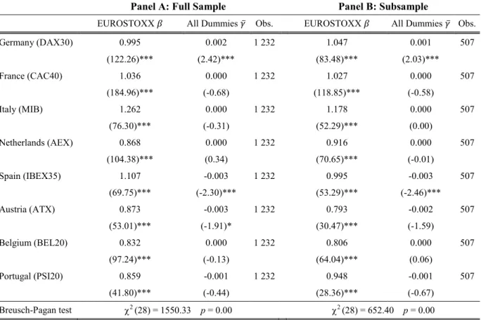
In this subsection, we apply the multivariate regression (2) to access the average abnormal variations in equity returns caused by both program announcement and launch. As proposed by Binder (1985), we apply a single dummy 𝛾̅ into the multivariate regression (2) that incorporates both announcement (PSPPa) and launch (PSPP1) at once, accessing the overall changes in equity markets. Table 5 shows the coefficient results from the eight European benchmark equity indices for both full sample and subsample periods.
In Panel A of Table 5, the overall results show that the European Quantitative Easing program seems to cause, on average, negative abnormal changes in 6 out of 8 benchmark equity markets, only statistically significant for Spain (IBEX35) and Austria (ATX) at 1% and 10% levels, respectively. The result is consistent with the recent study conducted by Assefa et al. (2016). In line with the isolated analysis of the program launch (PSPP1), here Spain (IBEX35) exhibits a negative average reaction in its benchmark equity index. Perhaps, the unstable political environment and associated uncertainty may be two relevant explanatory factors for the loss of Quantitative Easing program effectiveness, meaning that investors might not be willing to either invest or rebalance their portfolios during periods of instability.
Furthermore, in Table 5 the German index (DAX30) has a statistically significant positive abnormal return, at 1% level, consistent with Andrade et al. (2016). Although this positive reaction does not describe a clear path among most of the European equity indices, whether the portfolio rebalancing mechanism holds, it may evidence that German investors chose new asset classes (such as stocks or benchmark indices) due to the large liquidity available in markets.
Table 5 – Seemingly Unrelated Regression Model – Two-Step Estimator. This table presents the results from
the multivariate regression (2). This regression includes a single dummy 𝐷𝑎,𝑡= 1 for all days into the event
windows, each time we consider a related-event of European Quantitative Easing, and zero otherwise. The coefficient 𝛾̅ measures the average abnormal returns of each index i. In total, the model considers eight equations, different dependent variables (indices i) and the following independent variables: market portfolio (EUROSTOXX) and average dummy 𝛾̅. Panel A presents the results for the full sample from January 2, 2012 to October 31, 2016, that incorporates 1232 daily observations. Panel B presents the results for the same regression model, for a subsample from January 2, 2014 to December 31, 2015, that incorporates 507 daily observations. The eight country benchmark equity indices are the following: DAX30 is the German index, CAC40 is the French index, MIB is the FTSE MIB for Italy, AEX is the Dutch index, IBEX35 is the Spanish index, ATX is the Austrian index, BEL20 is the Belgium index and PSI20 is the Portuguese index. EUROSTOXX is used as a proxy for market portfolio. Both panels report regression coefficients as well as its t-statistics. The statistical significance levels are 10%, 5% and 1%, represented by *, ** and *** respectively.
Panel A: Full Sample Panel B: Subsample
EUROSTOXX 𝛽 All Dummies 𝛾̅ Obs. EUROSTOXX 𝛽 All Dummies 𝛾̅ Obs.
Germany (DAX30) 0.995 0.002 1 232 1.047 0.001 507 (122.26)*** (2.42)*** (83.48)*** (2.03)*** France (CAC40) 1.036 0.000 1 232 1.027 0.000 507 (184.96)*** (-0.68) (118.85)*** (-0.58) Italy (MIB) 1.262 0.000 1 232 1.178 0.000 507 (76.30)*** (-0.31) (52.29)*** (0.00) Netherlands (AEX) 0.868 0.000 1 232 0.916 0.000 507 (104.38)*** (0.34) (70.65)*** (-0.01) Spain (IBEX35) 1.107 -0.003 1 232 0.995 -0.003 507 (69.75)*** (-2.30)*** (53.29)*** (-2.46)*** Austria (ATX) 0.873 -0.003 1 232 0.793 -0.002 507 (53.01)*** (-1.91)* (30.47)*** (-1.59) Belgium (BEL20) 0.832 0.000 1 232 0.806 0.000 507 (97.24)*** (-0.13) (64.04)*** (0.06) Portugal (PSI20) 0.859 -0.001 1 232 0.948 -0.001 507 (41.80)*** (-0.44) (28.36)*** (-0.67) Breusch-Pagan test 2 (28) = 1550.33 p = 0.00 2 (28) = 652.40 p = 0.00
In conclusion, this incongruity among results indicates a non-regular path for general Eurozone countries, based on the analysis of benchmark equity indices. For instance, the
country reactions to the program may be justified by certain country-specific features, such as political, economic and banking regulations. Moreover, since financial markets are influenced by forward expectations, investor’s liquidity preferences and their levels of risk tolerance (Tobin, 1958), one might expect an early integration of the program’s information by investors and financial agents (Bernanke and Kuttner, 2004). Therefore, we assert that investors from countries in the Eurozone react differently to monetary policy shocks and, by this study, it is not possible to access the investment magnitude in equity markets as well as which potential changes occur in real portfolios’ composition.
5.4. Time-varying dummies
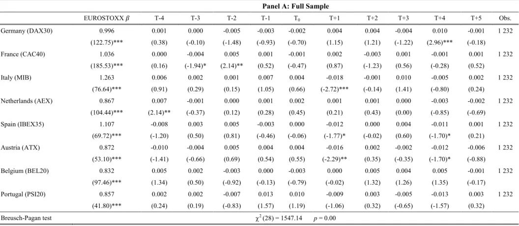
In this subsection, we present the results regarding the day-by-day analysis of equity abnormal returns for the European benchmark equity indices. Following the modified methodology applied by Rivolta (2014), we use 10 time-varying dummies into the multivariate regression (1) to access the abnormal changes in returns that may occur in each day of the chosen event window. For those dummies, the T-5 dummy is excluded to avoid potential collinearity problems. For each Quantitative Easing event (program announcement or launch), we jointly estimate the coefficients following the SURM, correcting for the potential presence of correlation between the countries’ residuals.
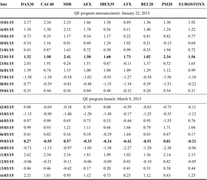
Table 6 shows the multivariate regression results from the modified model for the Quantitative Easing announcement, its levels of statistical significance as well as the Breusch-Pagan test of independence. For each day from January 15, 2015 to January 29, 2015 the model incorporates a dummy 𝐷𝑎,𝑡 = 1, excluding the day T-5, and zero otherwise. Overall, among all European benchmark equity indices, the path of the abnormal returns varies from index to index. For instance, there seems to be a negative reaction caused by the program announcement in the day T+1 for Italy (MIB), Spain (IBEX35) and Austria (ATX). For the German index (DAX30), it seems that a negative change occurs from T-2 to T0, indicating an anticipation from investors regarding the program announcement, yet not statistically significant. Contrary to portfolio rebalancing channel, perhaps investors kept on allocating the portfolio wealth in bonds or holding cash, yet not changing to riskier asset classes. However, this path changes after T0 until T+4 where positive abnormal change presents statistical significance, at 1% level. Also, for France (CAC40), it seems that T-3 and T-2 days are relevant in terms of abnormal variations in returns, however they are opposite in sign.
Table 6 – Seemingly Unrelated Regression Model – Two-Step Estimator by using Time-Varying Dummies for PSPPa event period. This table presents the coefficients
results from (1) obtained by following the modified methodology described in Section 3.1. Panel A presents the coefficients of a multivariate regression that includes 10 time-varying dummies and a proxy for market portfolio, for the full sample from January 2, 2012 to October 31, 2016, that incorporates 1232 daily observations. The time-time-varying dummies are considered from T-4 day to T+5 day. In detail, T-4 corresponds to January 15, 2015 and T+5 day is January 29, 2015. The eight multivariate regressions are jointly estimated. The eight country benchmark equity indices are the following: DAX30 is the German index, CAC40 is the French index, MIB is the FTSE MIB for Italy, AEX is the Dutch index, IBEX35 is the Spanish index, ATX is the Austrian index, BEL20 is the Belgium index and PSI20 is the P ortuguese index. EUROSTOXX is used as a proxy for market portfolio. The panel reports regression coefficients, its t-statistics as well as the Breusch-Pagan test of independence, distributed as a 2. The statistical
significance levels are 10%, 5% and 1%, represented by *, ** and *** respectively.
Panel A: Full Sample
EUROSTOXX 𝛽 T-4 T-3 T-2 T-1 T0 T+1 T+2 T+3 T+4 T+5 Obs. Germany (DAX30) 0.996 0.001 0.000 -0.005 -0.003 -0.002 0.004 0.004 -0.004 0.010 -0.001 1 232 (122.75)*** (0.38) (-0.10) (-1.48) (-0.93) (-0.70) (1.15) (1.21) (-1.22) (2.96)*** (-0.18) France (CAC40) 1.036 0.000 -0.004 0.005 0.001 -0.001 0.002 -0.003 0.001 -0.001 0.001 1 232 (185.53)*** (0.16) (-1.94)* (2.14)** (0.52) (-0.47) (0.87) (-1.23) (0.56) (-0.28) (0.52) Italy (MIB) 1.263 0.006 0.002 0.001 0.007 0.004 -0.018 -0.001 0.010 -0.005 0.002 1 232 (76.64)*** (0.91) (0.29) (0.15) (1.05) (0.66) (-2.72)*** (-0.14) (1.41) (-0.80) (0.24) Netherlands (AEX) 0.867 0.007 -0.001 0.000 0.001 0.002 0.001 0.001 0.000 -0.003 -0.002 1 232 (104.44)*** (2.14)** (-0.37) (0.12) (0.28) (0.45) (0.21) (0.43) (0.00) (-0.85) (-0.69) Spain (IBEX35) 1.107 -0.008 0.003 0.005 -0.003 0.000 -0.012 0.000 0.004 -0.011 0.001 1 232 (69.72)*** (-1.20) (0.50) (0.81) (-0.46) (-0.06) (-1.77)* (-0.02) (0.60) (-1.70)* (0.21) Austria (ATX) 0.872 -0.010 -0.004 0.005 0.004 0.004 -0.016 0.002 -0.002 -0.012 -0.006 1 232 (53.10)*** (-1.41) (-0.66) (0.69) (0.54) (0.55) (-2.29)** (0.35) (-0.35) (-1.70)* (-0.88) Belgium (BEL20) 0.832 0.005 0.002 -0.003 0.000 -0.003 0.000 0.005 0.004 0.005 -0.001 1 232 (97.46)*** (1.34) (0.50) (-0.92) (-0.13) (-0.79) (-0.02) (1.32) (1.26) (1.35) (-0.17) Portugal (PSI20) 0.857 0.002 0.002 -0.007 0.013 0.010 -0.009 0.003 -0.005 -0.013 0.003 1 232 (41.80)*** (0.24) (0.19) (-0.83) (1.57) (1.19) (-1.06) (0.32) (-0.65) (-1.57) (0.32) Breusch-Pagan test 2 (28) = 1547.14 p = 0.00
Table 7 shows the results from the multivariate regression that includes 10 time-varying dummies. Here, T0 is the day of the Quantitative Easing launch (PSPP1). The overall results lack statistical significance although there are unexpected results for certain indices. For the Austrian index (ATX), we find opposite signs in the reactions around the launch day, statistically significant at 5% level. Before the launch, the index reacts positively to the event while it reverses at the day T+1.
Additionally, the Portuguese index (PSI20) registers negative abnormal returns at the days T-3 and T+1, statistically significant at 1% and 5% levels respectively. Since the exposure of the Portuguese index (PSI20) to the European equity markets as well as to monetary policies in the European Union may be limited in comparison with higher traded indices in Europe such as DAX30 (Germany), one might suggest company-specific factors, other than the Quantitative Easing program itself, for the obtained negative abnormal variations in PSI20 index returns.
Overall, the results indicate a loss of power associated with subsequent events after the announcement of the Quantitative Easing program. According to Schweitzer (1989), the influence of subsequent events may persist even though the direction of returns (either positive or negative) lacks consistency.
5.5. Excluding the market portfolio
In this last subsection, we present the coefficient results for the multivariate regression (1), when excluding the market portfolio (EUROSTOXX) as an explanatory variable (𝑅𝑚,𝑡). Here, we intend to isolate the effect of the program and understand which variations are verified based on a single explanatory variable: The Quantitative Easing dummy (either PSPPa or PSPP1). We also do the process for the average multivariate regression approach (2). The chosen sample is the full sample from January 2, 2012 to October 31, 2016.
According to Panel A of Table 8 we find a clear positive reaction from the European equity markets to the Quantitative Easing announcement (PSPPa). For 5 out of 8 European benchmark equity indices, the abnormal results are statistically significant at 5% level. This abnormal change is supported and may be verified by the portfolio rebalancing channel where investors seem to be willing to shift their short-term asset allocations into riskier assets (as it may be the case of stocks or benchmark equity indices).
Table 7 - Seemingly Unrelated Regression Model – Two-Step Estimator by using Time-Varying Dummies for PSPP1 event period. This table presents the coefficients
results from (1) obtained by following the modified methodology described in Section 3.1. Panel A presents the coefficients of a multivariate regression that includes 10 time-varying dummies and a proxy for market portfolio, for the full sample from January, 2 2012 to October, 31 2016, that incorporates 1232 daily observations. The time-time-varying dummies are considered from T-4 day to T+5 day. In detail, T-4 corresponds to March, 2 2015 and T+5 day is March, 16 2015. The eight multivariate regressions are jointly estimated. The eight country benchmark equity indices are the following: DAX30 is the German index, CAC40 is the French index, MIB is the FTSE MIB for Italy, AEX is the Dutch index, IBEX35 is the Spanish index, ATX is the Austrian index, BEL20 is the Belgium index and PSI20 is the Portuguese index. EUROSTOXX is used as a proxy for market portfolio. The panel reports regression coefficients, its t-statistics as well as the Breusch-Pagan test of independence, distributed as a 2. The statistical significance
levels are 10%, 5% and 1%, represented by *, ** and *** respectively.
Panel A: Full Sample
EUROSTOXX 𝛽 T-4 T-3 T-2 T-1 T0 T+1 T+2 T+3 T+4 T+5 Obs. Germany (DAX30) 0.995 0.000 0.002 0.000 0.002 0.005 0.002 0.005 0.000 0.004 0.010 1 232 (122.58)*** (-0.08) (0.64) (-0.13) (0.70) (1.43) (0.74) (1.45) (-0.01) (1.29) (2.90)*** France (CAC40) 1.036 0.002 0.002 -0.001 -0.002 -0.003 -0.001 0.001 -0.002 0.000 -0.003 1 232 (185.19)*** (0.79) (0.85) (-0.63) (-0.71) (-1.44) (-0.57) (0.51) (-0.67) (0.05) (-1.24) Italy (MIB) 1.264 0.000 -0.003 -0.001 -0.001 0.008 0.002 -0.006 0.000 -0.010 -0.006 1 232 (76.47)*** (0.03) (-0.46) (-0.16) (-0.09) (1.23) (0.35) (-0.82) (-0.06) (-1.43) (-0.92) Netherlands (AEX) 0.867 -0.002 0.001 0.002 0.000 -0.002 -0.002 -0.001 0.000 -0.002 0.000 1 232 (104.31)*** (-0.65) (0.20) (0.60) (0.09) (-0.45) (-0.64) (-0.15) (-0.04) (-0.61) (0.11) Spain (IBEX35) 1.107 -0.002 -0.005 -0.005 -0.005 -0.001 -0.003 -0.013 0.000 -0.003 -0.007 1 232 (69.73)*** (-0.35) (-0.78) (-0.76) (-0.74) (-0.17) (-0.49) (-1.97)** (-0.05) (-0.43) (-1.00) Austria (ATX) 0.872 0.008 -0.011 0.008 0.015 -0.002 -0.014 -0.009 0.001 0.000 -0.008 1 232 (53.21)*** (1.20) (-1.63) (1.12) (2.21)** (-0.36) (-2.13)** (-1.27) (0.12) (0.05) (-1.24) Belgium (BEL20) 0.832 -0.003 0.003 -0.001 -0.001 -0.003 -0.004 -0.004 -0.001 0.000 0.001 1 232 (97.32)*** (-0.90) (0.89) (-0.23) (-0.32) (-0.95) (-1.13) (-1.21) (-0.15) (-0.10) (0.24) Portugal (PSI20) 0.858 0.006 -0.022 0.008 0.007 0.002 -0.016 0.003 0.009 0.000 -0.002 1 232 (41.94)*** (0.74) (-2.62)*** (0.97) (0.86) (0.22) (-1.85)* (0.35) (1.03) (0.00) (-0.28) Breusch-Pagan test 2 (28) = 1550.66 p = 0.00
Table 8 – Seemingly Unrelated Regression Model without the market portfolio – Two-Step Estimator.
This table presents the results of the multivariate regression (1), excluding the market portfolio EUROSTOXX as an explanatory variable for the eight European benchmark equity indices returns. Panel A presents the results for the full sample from January, 2 2012 to October, 31 2016, that incorporates 1232 daily observations. In total, the model considers 8 different equations, different dependent variables (indices i) and both PSPPa 𝛾1
(announcement) and PSPP1 𝛾2 (launch). Panel B presents the results for the same sample, applying the same
process described for Panel A. Here, there is a single independent variable: All Dummies 𝛾̅. The eight country benchmark equity indices are the following: DAX30 is the German index, CAC40 is the French index, MIB is the FTSE MIB for Italy, AEX is the Dutch index, IBEX35 is the Spanish index, ATX is the Austrian index, BEL20 is the Belgium index and PSI20 is the Portuguese index. Both panels report regression coefficients as well as its t-statistics. The statistical significance levels are 10%, 5% and 1%, represented by *, ** and *** respectively.
Panel A: Full Sample Panel B: Full Sample
PSPPa 𝛾1 PSPP1 𝛾2 All Dummies 𝛾̅ Obs.
Germany (DAX30) 0.008 0.006 0.007 1232 (2.12)** (1.51) (2.56)** France (CAC40) 0.008 0.002 0.005 1232 (2.18)** (0.48) (1.87)* Italy (MIB) 0.010 0.002 0.006 1232 (2.07)** (0.48) (1.79)* Netherlands (AEX) 0.007 0.002 0.005 1232 (2.13)** (0.74) (2.01)** Spain (IBEX35) 0.006 -0.001 0.003 1232 (1.34) (-0.12) (0.86) Austria (ATX) 0.003 0.001 0.002 1232 (0.69) (0.22) (0.64) Belgium (BEL20) 0.007 0.001 0.004 1232 (2.21)** (0.32) (1.78)* Portugal (PSI20) 0.006 0.002 0.004 1232 (1.55) (0.45) (1.41) Breusch-Pagan test 2 (28) = 23055.40 2 (28) = 23056.53 p = 0.00
In detail, for Germany (DAX30), France (CAC40) and Italy (MIB) we strongly point out the amount of cumulative monthly asset purchases as a plausible explanation for the positive abnormal returns around the announcement of the Quantitative Easing program (PSPPa). These three countries are highly exposed to the European monetary policies and may have strong equity market activity. These results are consistent with Andrade et al. (2016) who find higher stock prices in all European sectors after the policy announcement.
Although the results regarding the PSPP1 dummy (accounting for the launch of the program) indicate positive abnormal variations in returns, they are not statistically significant. This may be justified by the power of the event (higher in announcements) and by the portfolio
allocation near the announcement, thus not leading to a re-allocation around the Quantitative Easing launch period.
Panel B of Table 8 presents the results for the multivariate regression (2) with a single dummy variable 𝛾̅. This accounts for the average abnormal returns in benchmark equity indices when considering the dummy PSPPa (announcement) and PSPP1 (launch) into the regression, simultaneously. According to the panel, it seems that the program caused, on average, positive abnormal returns in the 8 European benchmark equity indices. The positive change is notorious for Germany (DAX30) and for the Netherlands (AEX), statistically significant at 5% level, and for France (CAC40), Italy (MIB) and Belgium (BEL20), statistically significant at 10% level.
Again, the Breusch-Pagan test of independence (3) with a p-value equal to zero shows the appropriateness of the applied methodology and the power in settling the heteroscedasticity statistical issue, emerged from event clustering.
Overall, by analyzing the four applied methodologies, the results show that countries with higher exposure to the program (such as Germany (DAX30), France (CAC40) and Italy (MIB))3 seem to react positively to the program, by both considering the announcement and the launch of the program. Moreover, although we do not measure the real magnitude of investors’ allocations into equity assets, we may suggest the portfolio rebalancing mechanism to support the positive market reaction in equity markets. On the other hand, we may identify political and company-specific issues, as well as unstable economic country environments, as potential explanatory factors for certain negative abnormal variations in country returns (such as for Portugal (PSI20), Spain (IBEX35), France (CAC40) and Austria (ATX)).
6 Further Research
While the effects of the Quantitative Easing program may seem to have both short-term and distinct impact on the economy, mainly due to the artificial creation of liquidity or notable through the portfolio rebalancing channel, a longer-term effect might emerge regarding asset allocation, readjustments in both risk and term premiums and, therefore, boosting the real effects for the economy. Although in the literature some authors point out the existence of portfolio rebalancing by investors in periods where Quantitative Easing program is either announced or launched, this mechanism may require longer periods of time to demonstrate consistence and a regular path from investors decisions.
A fact is that the program is still active in European markets and the economic effects are far from being presented in such a short measure of time. Therefore, the aim of this section is to provide some perceptions and mention further research regarding a longer-term analysis of the European Quantitative Easing program, enhancing the consistence of the results obtained in this study as well as the real effects observed in the economy.
There are some interesting stances that may be discussed and analyzed. First, one may try to understand whether the European Quantitative Easing program has a long-term influence on relative supplies of both monetary and real assets, rather than on aggregate demand (Tobin, 1969). Secondly, through a macroeconomic model of analysis, understand if the existent liquidity in the market (mainly held by national banks and other organizations involved in the program) causes positive effects in terms of demand for investment, consumption by individuals as well as by companies. Lastly, one may try to use the applied methodology in this study, with different event window and number of observations, in order to access comparable measures and improve the obtained results.
7 Conclusions
This study analyzes whether the Quantitative Easing program has an impact on European equity markets. The existing literature regarding this unconventional monetary policy covers its impact on bonds and on interest rates, since they are the most affected asset instruments by long-term asset purchases programs. However, little research has been focused on the impact of the program on the European equity markets. According to Bernanke and Kuttner (2004), monetary policy surprises are only liable on a cramped parcel of overall stock prices fluctuation, that may not be a priori an outcome from monetary policy effects on target interest rates.
Nevertheless, our study approaches the impact of the program on equity markets through benchmark indices. We consider the contributions of Binder (1985) and Pynnönen (2005) in the context of incorporation of dummy variables into the multivariate regression (MVRM). Due to potential issues regarding correlation between regression residuals and the presence of heteroscedasticity, a FGLS estimator is incorporated under the Seemingly Unrelated Regression Model (SURM). Then, we apply the methodology in four different forms with eight benchmark equity indices returns and dummy variables, depending on the event which is being analyzed.
Regarding the announcement of the program (PSPPa), it seems that positive abnormal variations in returns emerge for equity indices as a consequence of investors’ decisions around the announcement day. When excluding the market portfolio as an explanatory variable, we find evidence of positive abnormal returns during the Quantitative Easing announcement period (PSPPa) in 5 out of 8 European benchmark equity indices. One might recall the portfolio rebalancing mechanism (See Section 2) as the first channel whereby the investors shift the allocation of their assets in the portfolio by taking riskier positions in the markets. The results are supported by Joyce et al. (2011) and Andrade et al. (2016). The negative abnormal changes in returns are consistent with Assefa et al. (2016) and may be explained by the differences in country environments (including both political and economic issues) as well as the potential lack of effectiveness associated with the Zero Lower Bound (ZLB) environment.
Regarding the launch of the program (PSPP1), we find evidence of strong positive abnormal returns in DAX30 index (Germany) and negative abnormal returns in IBEX35 (Spain) and
CAC40 (France) indices. The first result may be associated with the exposure of the country to the large assets purchase program (See Table 9) while the second is associated with country politics (mainly Spain’s election in 2015). When excluding the market portfolio as an explanatory variable, the results lack statistical significance.
Lastly, although the Quantitative Easing program is a crucial influencer for the European financial markets, its long-term effects are problematic to identify by merely looking at backward data with little number of observations. Nevertheless, for the short-term analysis and apart from other macroeconomic factors, the program influences benchmark equity markets in the selected period of the events and the reaction from equity indices may depend on the countries exposure to the program.
8 References
Andrade, P., Breckenfelder, J., Fiore, F., Karadi, P., Tristani, O. (2016). The ECB's asset purchase program: an early assessment. European Central Bank. ECB Working Paper No. 1956, September 2016
Assefa, T., Esqueda, O., Mollick, A. (2016). Stock returns and interest rates around the World: A panel data approach. Journal of Economics and Business.
Bernanke B., Kuttner, K. (2004). What Explains the Stock Market’s Reaction to Federal Reserve Policy?. Federal Reserve Bank of New York Publications, March 2004.
Binder, J. (1985). On the Use of the Multivariate Regression Model in Event Studies. Journal
of Accounting Research. V23, 370-383.
Black, L., Hazelwood, L. (2012). The Effect of TARP on Bank Risk-Taking. International Finance Discussion Papers - Board of Governors of the Federal Reserve System, IFDP 1043.
Chen, H., Cúrdia, V., Ferrero, A. (2011). The Macroeconomic Effects of Large-Scale Asset Purchase Programs. Federal Reserve Bank of New York Staff Reports. Staff Report 527.
Claeys, G., Darvas, Z. (2015). The Financial Stability Risks of Ultra-Loose Monetary Policy. Policy Contribution No. 03, Bruegel.
Clarida, R., Galí, J., Gertler, M. (1999). The Science of Monetary Policy: A New Keynesian Perspective. Journal of Economic Literature. V37, 1661–1707.
Collins, D., Dent, W. (1984). A Comparison of Alternative Testing Models Used In Capital Market Research. Journal of Accounting Research. V22, 48-84.
Delivorias, A. (2015). The ECB's Expanded Asset Purchase Programme: Will quantitative easing revive the euro area economy?. European Parliamentary Research Service (EPRS). February of 2015.
Demertzis, M., Wolff, G. (2016). The Effectiveness of the European Central Bank’s Asset Purchase Program. Policy Contribution No. 10. Bruegel.
Gagnon, J., Raskin, M., Remache, J., Sack, B. (2011). The Financial Market Effects of the Federal Reserve’s Large-Scale Asset Purchases. International Journal of Central Banking. V7, 3-43.
Gambacorta, L., Hofmann, B., Peersman, G. (2014). The Effectiveness of Unconventional Monetary Policy at the Zero Lower Bound: A Cross-Country Analysis. Journal of Money,
Credit and Banking. V46, 4.
Harris, O., Huerta, D., Ngo, T. (2013). The impact of TARP on bank efficiency. Journal of
International Financial Markets, Institutions & Money. V24, 85-104.
Henderson, G. (1990). Problems and solutions in conducting events studies. The Journal of
Risk and Insurance. V57, 282-306.
Hyde, S., Bredin, D., Nguyen, N. (2007). Correlation Dynamics between Asia-Pacific, EU and US Stock Returns. In Asia-Pacific Financial Market: Integration, Innovation and Challenges, International Finance Review. V8, 39–61.
Joyce, M., Tong, M., Woods, R. (2011). The United Kingdom’s quantitative easing policy: design, operation and impact. Bank of England Quarterly Bulletin 2011 Q3. V51, 200-212.
Joyce, M., Miles, D., Scott, A., Vayanos, D. (2012). Quantitative Easing and Unconventional Monetary Policy – An Introduction. Royal Economic Society - The Economic Journal. F271-F288.
Keynes, J. (1936). The General Theory of Employment, Interest and Money. Edited by Palgrave Macmillan.
Kim, Y., Nam, J., Wynne, K. (2009). An event study approach to shocks in gold prices on hedged and non-hedged gold companies. Investment Management and Financial Innovations. V6, 112-119.
Knif, J., Kolari, J., Pynnönen, S. (2007). What Drives Correlation Between Stock Market Returns?. International Evidence. NBER Working Paper No. 8109.