Examining the relationship between time and factor anomaly returns

Examining the relationship

between time and factor

anomaly returns

Nuno Gontardo Vaz

Student Number 152417012

Dissertation written under the supervision of Joni Kokkonen

Dissertation submitted in partial fulfilment of requirements for the MSc in

Examining the relationship between time and factor anomaly returns

Nuno Gontardo Vaz

Abstract

By examining the return characteristics of 10 different, long minus short, accounting-based anomaly portfolios, we find that a portfolio that rebalances daily, based on either 10-K or 10-Q releases, is optimal when transaction costs are low (around 2% or less) and the anomalies are robust, with a 4.5% annualized return differential being created versus a yearly rebalance. However, when that is not the case, we find that a yearly rebalancing is best. Furthermore, we determine that no other common rebalancing periods (such as weekly) should be used as they consistently fail to outperform either the daily or yearly ones. We also find a significant clustering of anomaly returns around the release of 10-K and 10-Q financial statements, primarily up to 15 days, corroborating theories connecting news releases to anomaly returns. Nonetheless, we find anomaly returns to still be consistently present up to 365 days after a financial statement release, opposing the idea of fast market responses to information and large clustering. Overall, there appears to be a connection between anomaly returns and time considerations that warrants further study.

Keywords: Rebalancing, factor investing, anomalies, abnormal returns, market efficiency.

Examinando a relação entre tempo e retornos de factores anormais

Nuno Gontardo Vaz

Resumo

Ao examinar os retornos gerados por 10 portfólios de anomalias baseados em factores contabilísticos, e que são “long” menos “short”, concluí-se que um portfolio que faça rebalanceamento de forma diária, com informação de um formulário10-K ou 10-Q, tem uma desempenho melhor que um que faça o mesmo, mas anualmente, quando os custos de transacção são baixos (por volta de 2%) e as anomalias são robustas (com uma diferença, média anual, de retornos de 4.5% entre um e o outro). Nas situações em que isto não acontece, o rebalanceamento anual é superior. Para além disso, concluí-se que nenhum outro método de rebalanceamento comum (como por exemplo, semanalmente) deve ser usado, pois não demonstram um desempenho melhor que o método diário ou anual. Nesta análise, também encontramos evidência de um agrupamento de retornos de anomalias à volta da disponibilização de informação (para os formulários 10-K ou 10-Q), particularmente até 15 dias após esta ocorrer. O que corrobora as teorias que conectam a disponibilização de informação ao mercado com retornos associados a anomalias. De qualquer modo, verificamos que os retornos de anomalias continuam a ser consistentes até 365 dias após a informação ser disponibilizada, o que contradiz a ideia de um grande nível de agrupamento nos retornos e de uma resposta rápida e eficiente, pela parte do mercado, à nova informação. De forma geral, existe evidência de uma ligação entre retornos de anomalias e tempo que exige maior estudo.

Palavras-chave : Rebalanceamento, investimento factores, anomalias, retornos anormais,

Acknowledgments

In this section, I wish to thank and acknowledge individuals who have not only, directly, helped in the development of this dissertation by providing ideas, reviews, suggestions and comments but also those who, through personal support, have also, indirectly, contributed.

First, and foremost, I wish to thank Professor Joni Kokkonen, my thesis supervisor, who was always supportive and helpful during the entire process. Thank you for always being available for meetings, discussions and reviews and for guiding me throughout the thesis with numerous suggestions, corrections and constructive criticism. I always felt that I had support and that is incredibly important.

A thank you to Simon Schmidt, a friend and mentor during my summer internship, who first introduced me to the research papers on which this study is based and which first suggested and discussed with me the primary investment strategy idea present in this dissertation.

A thank you also to my parents and aunt who were incredibly helpful, encouraging and motivating during my research and throughout my life. Their never-ending support, love and availability is incredibly important to me.

A final appreciation note to the Fundação para a Ciência e a Tecnologia (FCT) for the financial support.

1

1. Introduction

Recent academic research, in asset pricing anomalies, has corroborated the theory that the existence of factor anomalies is closely related to the release of news or information. The idea being that the abnormal returns identified, for example around earnings announcements, could reflect market mispricing, with investors having biased expectations which are corrected as the information is released to the public. Engelberg, McLean and Pontiff (2017) have recently studied this argument, by analysing more than 6 million news days and their respective abnormal returns. They concluded, firstly, that anomaly returns are, on average, 6 times higher on earnings announcement days and 50% higher on corporate news and that this effect is mainly due to investor’s biased expectations being corrected as news arrive. Secondly, they also found that analysts typically overestimate earnings for short anomalies portfolios and underestimate it for long portfolios (explaining the success of these factor portfolios in capturing abnormal returns). Their personal theory is that all forms of news can potential create anomaly returns, as long as their arrival can correct those biased beliefs held by investors, but with earning’s announcements being more significant than any others.

As a follow on, a working paper by Bowles, Reed, Ringgenberg and Thornock (2018), finds that anomaly returns are earned, almost exclusively, around the release of information, in particular in the first 30 days and mainly for information regarding fundamentals. They also find that hedge funds which are quicker to react to this information have greater abnormal returns, suggesting an idea of quickness as a factor in earning abnormal returns. Finally, they conclude by suggesting that anomalies should not be thought of as buy-and-hold portfolio strategies but as trading opportunities, happening around the release of information, and that, contrary to Engelberg et al (2017), not all information releases create anomaly returns but only that which drives the formation of these same long-short anomaly portfolios.

This dissertation research can be seen as a complement to these two above-mentioned papers, in particular the one by Bowles et al. (2018), on whose methodology it is grounded. The objectives here can then be divided into two lines of research. To, firstly, examine whether there truly is a robust connection between the release of information and factor anomaly returns and a significant degree of concentration and dependence on time (by investigating the time profile of these abnormal returns around news release days), in particular, for the publishing of financial statements (namely 10-K and 10-Q, which are the annual report and the quarterly report respectively) and their effects on 10 different accounting-based anomaly factors. While,

2 the second line of research, is to test the practical validity of these same 10 accounting-based anomaly factors as investment strategies, by building on the idea of “trading opportunities happening around the release of information” and focusing on short rebalancing timeframes around 10-K and 10-Q financial statement releases, rebalancing up to daily to try and quickly update anomaly portfolios to capture these “bursts” of abnormal returns. The idea here being to identify which form of rebalancing is best, for this particular task, and, in particular, when a transaction cost trade-off is introduced.

For the first line of research, an analysis, similar to an event study, is constructed, with stocks that had a financial statement release which would warrant their admission into an anomaly portfolio, throughout a 20 year period, being added to a portfolio which averages their returns up to the 365 days, with point zero being the news release day. The idea here being that days which are closer to point zero should outperform those days that are farther away in time. This analysis finds that is the case, at least up to the 15 days point, with the 1 day and 7 day point being particularly strong, in this regard, as they present a 14.9% and a 5.8% annualized return spread versus the 365 day point when in a combo portfolio (a portfolio that merges the 10 anomalies together). This also means that, past the 15 day point, abnormal returns are generally earned in a quite consistent fashion up to 365 days past a financial statement release. These results are present even when the periods are analysed independently of each other or when they are compared in cumulative terms.

On the other hand, for the second line of research, different anomaly investment strategies, with multiple rebalancing intervals (of daily, 7 days, 15 days, etc.) are backtested for the 1996 to 2017 period and their returns compared, with and without transaction costs, as to see which ones perform the best. Findings are that a daily rebalancing strategy, which combines the 10 anomalies into a combo portfolio, outperforms the same one but rebalancing annually by a 4.5% spread of annualized return, averaged over 20 years. These findings are also, mostly, consistent for the individual themselves and are particularly strong for those anomalies which relate to profitability, such as return on equity which features a 9.7% spread.

When transaction costs are taken into account, however, these profitability related anomalies are the only ones which consistently continue to outperform the yearly rebalancing, showing that a daily rebalance can only provide outperformance, when transaction costs are accounted for, if the anomalies are sufficiently robust and the transaction costs are low to moderate. It is also determined that other rebalancing periods, besides daily and yearly, are mostly irrelevant

3 as they fail to outperform either one consistently (with the best form of rebalancing being daily, when there is confidence in the robustness of the factor strategy, or yearly if that is not the case). This paper, from here on, is then divided into 4 major sections. Background & Literature Review, where more information is given as to the history behind these questions and the academic literature that exists surrounding them. Data & Methodology, where the databases used, and their construction, is described in detail as is also done for the two types of studies that have been referred to above. Empirical Results, which comments and analyses the findings that come from these studies and is divided into two sections, one for each study. And, finally, Conclusions, Limitations and Future Research where the results are presented in a more condensed form with notes as to potential limitations from them and ideas for future lines of research.

4

2. Background & Literature Review

This paper is associated with the broad literature on the topic of asset pricing anomalies, as such, an overview of the subject matter and its most current developments is presented as a preamble to the research.

An anomaly is habitually defined as an abnormal return event that is outside of what is predicted by financial models (such as the CAPM or the Fama-French model) and whose empirical testing results are divergent from what is to be expected from the risk-return relationships implied by these models (e.g. they produce an “alpha”, an excess risk-adjusted return). These abnormal returns, if they are to exist, contradict, partially, the efficient-market hypothesis (or might indicate the use of an incorrect equilibrium model) and, if exploited, may allow for market outperformance. Usual examples of anomalies are the January effect (where stocks that underperform in the last quarter over perform in January of the following year) and the size effect (smaller firms typically outperforming larger firms). At least more than 300 such anomalies have been identified, according to Harvey, Campbell, Liu, and Zhu (2015), and economic theory would imply that once these anomalies are acknowledged, their magnitude should decrease as investors seek to exploit them. While some papers find this to be true for some anomalies, other studies show that the majority of anomalies are persistent. For the reasons above, there is a great deal of interest surrounding the study of anomalies in academia and a significant debate as to whether these anomalies do in fact exist, their persistence and the extent of their effects.

Seminal papers that focus on the topic of asset pricing anomalies include Ball & Brown (1968) which pioneered the study of anomalies by first establishing a relationship between accounting net income and abnormal returns and Fama and MacBeth (1973) which developed the use of regressions on risk factors to evaluate market efficiency and first established market beta as a factor in predicting returns. Banz (1981) first discovered the size factor effect by finding that small stocks (by market capitalization) have abnormally high average returns when compared to larger ones. Basu (1977) finds that stocks with low relative price to earnings ratio outperform those with higher. Fama and French (1992) and Carhart (1997) introduce common factors models, based on these newly discovered anomalies and the arbitrage pricing theory (APT), to better capture new risk premium.

5 However, even though there are more than five decades of research into the topic, definitive answers for the drivers of these anomaly returns are still inconclusive. There are, commonly given, explanations that are not, by themselves, necessarily mutually exclusive nor exhaustive. Firstly, there is the possibility that these anomalies are the result of differences in risks, which will be reflected in the discount rates that were used to value the assets in the first place, but that are not being actually modelled. An example of this is the paper by Bansal, Dittmar and Lundblad (2005) which finds that 62% of the variation in risk premium, across 3 anomalies, can be explained by the cash flow beta (which is a measure of cash flow risk) and which is not usually accounted for in models (such as the CAPM). The logic being that, as asset prices reflect the value of the discounted cash flows, the cash flow risk should have some bearing on the total risk compensation of the asset.

A second explanation, is linked to market inefficiency from behavioural biases and biased expectations from investors. If investors in a market were to have biased expectations on information, such as cash flows, and a specific anomaly was correlated to this then the arrival of new information, for example on the release of a 10-K, would lead to a price correction and an abnormal return for this anomaly’s portfolio. Recently, Engelberg, McLean, and Pontiff (2017) examine this connection between information release and anomaly returns by comparing news release days against non-news days. They find that on corporate news release days abnormal returns are 50% higher and, on average, 6 times higher on earnings announcement and conclude that this effect is mainly due to biased expectations and the following price corrections on information arrival.

Other potential explanations, are the existence of a time-varying risk premium which can be forecast, and therefore w ill show correlation to anomaly portfolios, but only due to the state of the macro economy, not due to any understanding on the future behaviour of stocks, and, therefore, will not allow you to consistently profit. A final explanation can also be the existence of limitations (including simple trading costs) to arbitrage that simply do not allow the anomalies to be exploited in practice as they are studied in theory.

While, as described before, there is academic agreement and confidence in the existence of anomalies, some more recent academic developments have also brought into question the idea of robustness, in itself, for most of the recently discovered anomalies, mostly due to the application of a more rigorous set of statistical tests and methods than before. With the idea being that most anomalies originate from data mining and the data-snooping of fixed datasets.

6 Harvey et al. (2015), for example, tests more than 300 anomalies proposed in the last decades, and concludes that “most claimed research findings in financial economics are likely false” arguing that “it is a serious mistake to use the usual statistical significance cuoffs (e.g., a t-statistic exceeding 2.0) in asset pricing tests”. This, he says, because finance is working with very limited datasets and, therefore, data mining is a very prevalent issue. The paper recommends “a t-statistic of 3.0 (which corresponds to a p-value of 0.27%)” as a minimum to properly conclude on the significance of an anomaly. As a follow on, Hou, Kewei, Xue, and Zhang (2018) apply these more rigorous statistical testing hurdles to 452 anomalies and find that “most published U.S. stock market anomalies are not replicable after reasonably demoting microcaps to a very minor role, and especially after raising the threshold for significance to account for data snooping”. Of the 452 anomalies presented, 65% cannot clear the previous 1.96 t-value standard and 82% fail a 2.78 test hurdle. They find that the well-studied anomalies, such as value, momentum, investment or profitability, replicate well, while others, such as trade frictions, do not. The conclusion being that “capital markets are more efficient than previously recognized” since very few of the studied anomalies actually are significantly present in the data but that the existence of some anomalies, by themselves, is not yet ruled out.

Lu, Stambaugh, and Yuan (2017) decides to better verify the idea of robustness in some anomalies by looking at “a pre-specified set of nine prominent U.S. equity return anomalies” and find that all of them also produce significant alphas in Canada, France, Germany, Japan, and the U.K which goes against the general idea of data mining and corroborates the idea of some anomalies being consistently significant (since these are less commonly used datasets). A similar paper by Hanauer and Lauterbach (2018) further tests a broad set of anomalies on 28 emerging countries and finds that “variables of the categories value, profitability, and investment, but also momentum, exhibit t-values of the long-short hedge portfolio returns well above 2”, further strengthening the idea of robustness for some anomalies.

As for accounting anomalies in specific, the current literature is similar in its conclusions. Linnainmaa, Juhani, and Roberts (2016) report that “the majority of accounting-based return anomalies are most likely an artifact of data snooping” when examined out-of-sample. However, once again, the paper still finds that some of the main accounting anomalies, such as accruals, growth in inventory or profitability appear conclusively robust. Other papers corroborate this idea, for example, Green, Hand, and Zhang (2017) who study 94 accounting anomalies and find that 12 are robust to data-snooping.

7 Consequently, and as a summary, academic literature appears to be in agreement in three primary notions. Firstly, in an increasing scepticism towards the bulk of recent anomaly results and the demand for higher quality statistical criteria before result presentation so as to increase its own credibility. Secondly, in the idea that there are some anomalies which are persistently present and therefore are worthy of further study. And, thirdly, in the lack of a definitive answer as to what concrete phenomenon is behind the existence of those anomalies that are indeed deemed robust.

8

3. Data & Methodology

As mentioned in the introduction, this paper focuses primarily on two axis of research. Firstly, through an event type study on the cumulative anomaly portfolio return, an analysis as to the connection between news information release dates and anomaly portfolio assignment, as a potential explanation for the anomaly factor returns and the clustering of abnormal returns near these news days, identified in Engelberg et al (2017). Secondly, examining both the importance of different rebalancing periods in the accumulation of abnormal returns and their viability as investment strategies, and the possibility of improving them, by comparing the returns from investment strategies with the same anomaly factors but different timeframes.

For both of these lines of research, there is a need to define a news information release date (a signal) and its relationship to the anomaly portfolios. Therefore, market-based anomalies, such as size, have to be excluded as they are continuously updated. The same can be said for behavioural anomalies, such as the January effect. Accounting-based anomalies are, then, the natural choice. The two most significant accounting-specific news information releases, per Engelberg et al (2017), that can be known beforehand, are earnings announcements and financial statements releases, in the form of a 10-K (annual report) or a 10-Q (quarterly report) which are company specific financial statements that are mandatory for public companies to be filed with the Securities and Exchange Commission (SEC). However, earnings announcements do not have a predefined set of information that is to be released (some companies may release more information than others) and are typically lacking in information (only presenting some key values), as such, they are not adequate for this type of analysis (which relies on a set date and a set number of key accounting values). Financial statement releases are, hence, the most adequate option, in particular because as of their release date we can be sure that all data for our anomaly portfolios is available to the market (since there is a pre-set legal requirement, for public companies, by the SEC, to present certain data such as revenues, inventories, profits, etc.) and, therefore, that portfolio reassignment will happen, which leads to a more robust study as there is a smaller risk of our anomaly portfolios anticipating the market (by investing using information not yet available to the public). Financial statements release dates are also easily identifiable and available to the public at no cost or friction (and this is true even before they occur).

Since Compustat is missing K filing dates, there is a need to compile a proper dataset on 10-K release dates from other sources. For this, two different datasets were collected and merged

9 (as to minimize any potential for missing dates). The first dataset is a compendium of 10-K filing headers, for public companies, provided by Bill McDonald in his website1 _{(from which}

release dates can be extracted). The second dataset is similar, also containing header values, and is provided by the WRDS repository2_{. Dates are available for the period from 1994 to 2017.}

Since both these datasets contain a CIK number (a SEC identification number), which is also available on Compustat, a connection is then possible to be drawn between the two datasets based on this CIK number and the fiscal year of the financial statement data available in both Compustat and the datasets. Proper checks where run to confirm that no dates were replicated and that no more than one set of financial information was available for each fiscal year. As for 10-Q release dates, they are available in Compustat, under the FDATEQ variable. However, this variable is severely lacking in data and, therefore, there was a need to find an added solution. The variable RDQ was also used, which stands for the report date of earnings, and a delay of 20 trading days (approximately equal to one month) was used as to avoid any look-ahead bias. With the average gap between earnings release and financial statement being of just 4 days, we feel this is a conservative approach.

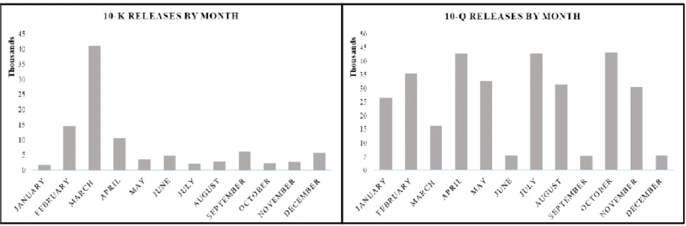
Figure I: Total number of financial statements (left is 10-K and right is 10-Q) used in

calculations by month of release.

Since stock return data is also needed, the CRSP database is used. To connect the Compustat and CRSP databases to the 10-K dates, PERMCOs are associated to the CIK numbers. Values from 1994 to end of 2017 are retrieved. Data filtering is done on both of these databases to ensure proper values. For the Compustat data, revenue, total assets, net income must exist, as well as an associated fiscal year/quarter. Afterwards, if any of the essential components of a

1 _{https://www3.nd.edu/~mcdonald/}

10 particular anomaly calculations are missing, for example missing equity when calculating return on equity, the particular stock is ignored. For the CRSP data, stocks with price below 5$ are removed, only NASDAQ, AMEX and NYSE exchanges are considered, share codes are restrict to 10 and 11 (common stock), and shares outstanding must be above 10 million. When it comes to daily holding returns retrieved from CRSP, any further computation involving returns on news days only considers the holding period return from the day after (which is the return from price close from the news day to close to on the day after) so as to be precautious and ensure there is no risk of anticipating the market, and creating an overestimation of the anomaly effects on returns, by having information that is not yet available to the public being present in portfolio choice. Finally, data above the 98th _{or below the 2}nd _{percentiles (for CRSP}

daily holding period returns) are also removed to further safeguard the analysis from the effect of overtly strong outliers or incorrect CRSP data.

The subsequent phase in the study is the construction of the anomaly portfolios. As to the anomalies themselves, due to the data mining concerns discussed in the background section, it is best to select anomalies which have a robust and well-established academic history and which change at a distinct and specific observable point in time (matching with the 10-K or 10-Q financial statements release, from which the necessary data is available). The final 10 anomalies selected were based on the Bowles, Reed, Ringgenberg and Thornock (2018) working paper, and their corresponding reference papers, but may not necessarily follow the same construction method. The specific methodology for each anomaly’s calculation is described in Table I. After the calculation of each of these 10 anomalies, the underlying stocks are ranked (a relative rank based only the anomalies themselves) and then divided into deciles. The long and short portfolios will be defined based on either the 1st or the 10th decile, depending on the specific anomaly in question, as detailed in the Table I descriptions. For example, the long portfolio for the Accruals anomaly will correspond to the 1st _{decile, which matches the lowest values, and}

the short to the 10th _{decile. It is also important to note that, for all cases, the portfolios are strictly}

built on an equal-weight basis and so is any form of return calculation presented in this paper. At this point, there is a split in the methodology, between the two lines of research mentioned in the first paragraph of this chapter. Any methods mentioned beforehand are equal, for the two. We begin with the methodology for the second mentioned analysis topic: the studying of rebalancing portfolio investment strategies, for different time period intervals of 365, 180, 90, 30, 15, 7 and daily, and with including potential transaction costs. A starting portfolio, for each

11 anomaly and each time period interval, with the same construction methodology as mentioned beforehand, is formed on the first trading day of 1996 (so as to have 2 years of accumulated financial statement data). Afterwards the portfolio is rebalanced according to its respective time interval. This means that, for example, the daily portfolio may be rebalanced in the second trading day of 1996 but that will only happen if there are any new stocks that have an information release and entered either the top or bottom decile. If that is not the case then the portfolio is not altered. This is a continuous approach. The 7 day portfolio, on the other hand, works the same but may be rebalanced only once one week passes (regardless of whether it is rebalanced or not, another week must be waited) and so on for the other time intervals. The rebalance dates are select as being the trading day closest to the timing schedule (so if, for example, after waiting one month, for the 1 month rebalance strategy, the rebalance date ends up on a Sunday, the rebalancing date is pushed to Monday). The only time interval that is handled slightly different is the 365 days interval, which is rebalanced on the last trading day of June of the respective year and, therefore, does not start in the first trading day of the year. This is to ensure that the yearly rebalancing portfolio is working on optimal settings, for fair comparison, as June is the typical rebalancing month for yearly portfolios used in prior research. A “combo” portfolio, which aggregates the 10 anomaly portfolios by equal-weighting them, is also present, for each time interval.

This portfolio building strategy is now repeated, in the exact same fashion, but in a way which accounts for transaction costs (so as to achieve a more practical threshold and to compare results between the two). For these transaction costs, an approach was chosen based on academic research. Lesmond, Ogden and Trzcinka (1999), a common academic source for these types of estimations, finds that transaction costs typically range between 1% of stock market value, for high market capitalization stocks, to 10% value, for the lowest. However, this paper was also published two decades ago and transaction costs have significantly decreased with the increase in electronic trading. Edelen, Evans and Kadlec (2013), for example, find an average of 1.4% transaction costs for mutual funds in the US. Therefore, a decision is made to assume that the total transaction costs (buy and sell included) are a fixed 2% market value of the stock. If the rebalancing strategy entirely fails to hold even in these beneficial standards, then it may be dismissed, otherwise it may be deemed worthy of further study. This means that, in practice, each time a new stock enters the anomaly portfolio (long or short) 2% of market value for that stock is immediately removed creating a more immediate trade-off for the portfolios with shorter rebalance intervals.

12 Finally, as an added study, a portfolio that goes long in the daily rebalancing portfolio (which itself is the long-short portfolio for the anomaly) and shorts the yearly portfolio (which is also long-short) is also examined through the 1997 to 2017 period, without transaction costs. The point here is to better scrutinize whether there is a sufficiently significant return spread, not just as a final average but throughout the whole period, between the common yearly form of anomaly portfolio rebalancing and this, more continuous, form of daily rebalancing. If no such spread exists for the more active form of rebalancing, daily, then we can conclude that yearly rebalancing is likely optimal. This same portfolio’s returns are also regressed on the five Fama-French Factor models to examine, firstly, if there is “alpha” creation for the daily vs yearly rebalancing (meaning that a portion of the returns cannot be explained by these commonly factors) and to examine, for each anomaly, their correlation to these same explanatory factors. Now, we move on to the event time type study, which was the first one mentioned in the introduction. Some methodology aspects are similar but not identical. Firstly, the factor deciles are built in the same way. Nonetheless, the event time anomaly portfolios now only accounts for the returns from stocks that have an information release that leads to a stock being in the top or bottom decile (in the rebalancing portfolios all stocks on the top and bottom deciles are accounted for, not only those that had a news release on that date). That is to say that once a stock enters a long or short portfolio, its returns are lined up in event time, with the information release date being date zero for this stock. This way, only the return effects that are directly connected to the release of information are considered. Also, important to mention, is that while the time intervals are the same as for the rebalancing portfolios, in this particular case they represent the length of time that the returns are accumulated for and not the rebalancing time interval. This means that, for example, if a stock has a news release that puts it into the top decile the 365 days portfolio represents the accumulated returns for that stock for the next 365 days while, for example, the 7-day portfolio will only consider it for the following 7 days. Comparison between the 365 days and the shorter time period portfolios will allow to draw conclusions as to how much of the anomaly abnormal returns are received in each specific timeframe. The greater the significance of the shorter period portfolios the greater the connection we can draw between information release and abnormal returns.

As a final note, it is important to mention that there are, for both of these studies, small differences between the 10-K and 10-Q sections, such as the 10-Q naturally having more data points than the 10-K, but, irrespective of this, the methodology described above is practically identical for both.

13

4. Empirical Results

This section now comprises the results from the whole research and is divided into 3 parts. The first part, which is this one, discusses figures that are general to both studies (such as the standard deviation of the anomaly values). The two other parts, particularize on their respective studies.

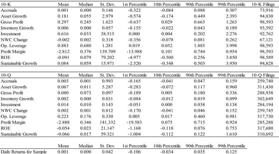
In Table II summary statistics for the 10 studied anomalies are presented, as well as for the daily holding period returns used throughout the study. From 1994 to 2017 there are 7103 different stocks used, with the average number of total 10-K filings utilized being around 90,000 and the average for 10-Q being around 293,000 (the differences in the number of information releases, for each anomaly, come from some 10-K or 10-Q having missing values).

In regards to the anomaly factors themselves, in Table II, there is a large parallel between summary statistics for the 10-K and 10-Q statements, which is to be expected and demonstrates data consistency across the two study sections. The average firm appears to have strong operational losses as the average profit margin, of -280%, is significantly negative, however the median is surprisingly positive, at 37%, showing that the most likely scenario is for a small portion of outlier firms being severely unprofitable. The same is true for return on equity. This will be relevant, later on, as a large part of profitability related anomaly returns are based on the short component. Discrepancies between 10-Q and 10-K statements for factors that use income statement items, such as operating leverage, can be explained by the fact that the 10-Q will only show income statement data for a quarter while 10-K will do it for a year. The factors relating to working capital (namely Accruals and NWC Change) also appear with mean and median close to zero, which may mislead into thinking that these suffer from data problems but this is not the case but simply the fact that the changes in percentage are typically small and equally distributed on both the positive and negative sides leading to averages near zero. Asset growth suffers from a quite strong standard deviation, of more than 200%, mostly due to the fact that the firms present in the data are not separated by size. Therefore, you will typically have the smaller firms having asset growths on a much larger scale than the bigger, well established firms, which also means that both the long and short portfolios for asset growth are likely to contain small size firms as they are much more likely to have extreme values.

Also in Table II, the bottom row is “Daily Returns for Sample” which is summary statistics for the entire sample of daily holding period returns retrieved from 1995 to 2017. The average daily return for this dataset is 0.1%, which may appear small but corresponds to a 25% annualized

14 return. The median return is also positive but smaller. On the other hand, a 4.2% daily average standard deviation represents an annualized standard deviation of 66%, a somewhat high value. Nonetheless, these represent a Sharpe ratio of approximately 0.4, which is in line with the usual values for the market.

Bowles, Reed, Ringgenberg and Thornock (2018) whose methodology this paper is based on, also present a sample summary statistic for their anomalies, albeit only using 10-K statements (in their paper they only use 10-K). So, a comparison is easy to make between the two. In general, most statistics are very similar between both researches which is a good sign for data consistency. For example, their 1st _{and 99}th _{percentile for daily returns, for the whole sample,}

are -9.38% and 10.64% while this paper’s are -10.6% and 12.5%. Profit margin on average, in their research, also have a similarly strong negative bias of -373%. And, overall, profitability anomalies match in their extremeness. A few of the significant differences that are worth pointing out are in the asset growth anomaly, which has a much lower standard deviation of 38%, albeit mean and median are similar, and in the investment anomaly which has a significantly higher mean of 1.1 versus our own 0.6 value.

4.1 Empirical Results – Investment Strategies

This part now contains the results from the different time intervals rebalancing investment strategies discussed in the methodology section. This is the strategy that forms anomaly portfolios based on going long or short on the top and bottom decile and then rebalances according to a pre-defined interval schedule (daily, 7 days, 90 days, etc.) therefore updating for any releases of information that may affect the extreme deciles. The strategies are backtested from 1996 to 2017. All 10 previously mentioned anomalies are shown and a “combo” portfolio, of the 10, is also formed, based on equal weighting the 10 anomalies. Here, as discussed before, the objective is to accept the assumption that anomaly abnormal returns are clustered around information release and see how good strategies which take more immediate advantage of information release are, in practice, when compared to slower updating periods at capturing abnormal anomaly returns. Firstly, by examining without considering for transaction costs and, then, with estimations for transaction costs as these will be very relevant for practical implementability.

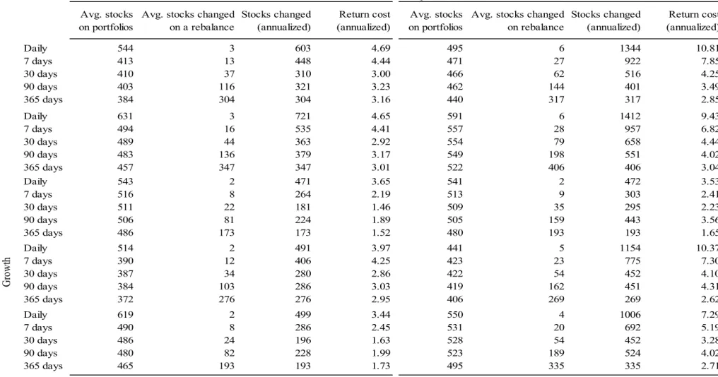
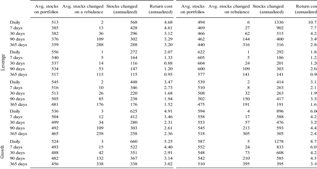
15 As a preliminary to the discussion on the results of the investment strategies, Tables III and IV are auxiliary tables that contain important summary information for understanding the rebalancing methods and, from these, the estimation of transaction cost (which will be used in the investment strategies). Shown are the number of stocks that are in both the long and the short anomaly portfolios together (on average) as well as information on the number of stocks bought, on average, in each rebalance, result which is then annualized to better compare between strategies. Finally, transaction costs incurred in the form of lost return, by rebalancing the portfolios, are also shown in annualized terms (meaning the cost for a whole year of rebalancing the portfolio using the specific time interval). From these tables, we can conclude, firstly, that the average number of stocks held at a random point in time is around 470 for the 10-K strategies and slightly higher for the 10-Q, at an average of 500, which implies well-diversified portfolios, at all points in time. Secondly, that, on average, the number of stocks bought is slightly greater for the 10-Q section and that this number is usually increasing with the increase in time between rebalances, as it is expected, although the 365 days timeframe, which as detailed in the methodology section rebalances only on end of June, may frequently rebalance more than the 90 days one, in annualized terms. The asset growth anomaly appears to be the one of the most rebalanced with an average of 1412 stocks bought per year for the daily strategy, potentially due to the already discussed high volatility in asset growth values for the dataset, while operational leverage is the opposite with only 292. Thirdly, transaction costs do typically have a negative correlation with the length of the timeframe, as it makes sense, but this is not a linear relationship as the daily and 7 day rebalancing are exponentially more costly while the remaining strategies are closer together in cost (potentially due to the discussed clustering in the financial statement release dates). With the cost up to 90 days often only being slightly different from the 365 ones in the 10-Q section (probably due to the 10-Q being released quarterly). This is interesting as there may be an optimal inflection point between the extra returns from shorter timeframes rebalancing and the extra costs from such rebalancing. As an example, the yearly portfolio ends up changing an average of 58% of its stocks, each year, while the 90 days portfolio, for example, changes 62%, on an annualized average. Not a large and significant difference. The average yearly transaction cost for the daily rebalancing appears to be around 7% for the 10-Q section and 4% for the 10-K while for the 365 rebalance it is only around 3% and 2% respectively. A significant difference. However, if we compare with the 90 days, which have transaction costs of 3.7% and 2.5% respectively, the difference is much smaller.

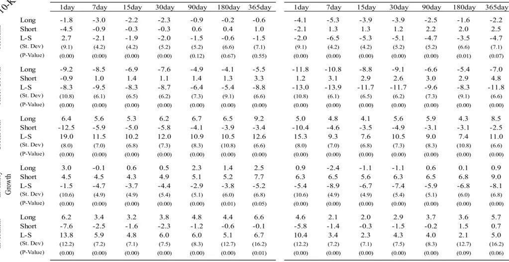
16 Now, we examine the results from the investment strategies themselves, which are present in in Tables V to VI. Of these four tables, the first two use 10-K statements to rebalance while the last two use 10-Q statements. Each strategy is parted into its long and short component, to better understand the source of returns, and the final, long minus short, is also shown. For these, the results are given as absolute annualized daily return averages, for each respective time period (shown in the header row). A standard deviation, for the final long minus short component, which is similarly annualized and in absolute terms, is also presented. Finally, a p-value is calculated as to determine the significance of the long-short anomaly portfolio results when compared with a 0% return. Each table is split in two, with the left-side having the strategies with transaction costs being ignored, and the right-side having transaction costs being taken into account (as detailed in the methodology section).

If, for now, we ignore transaction costs (meaning that we only look at the left-side panels of these tables), an immediate overview can be had by looking at the combo strategy (which is on the bottom left corner of Tables VI and VIII) and seeing that, without transaction costs, the daily strategy outperforms any other rebalancing interval by a considerable margin, in particular, the daily strategy returns 9.0% for the 10-K and 7.7% for the 10-Q while, for example, the annual rebalancing only returns 4.5% and 5.5% respectively. And, this, without producing significantly more standard deviation, 9.2% for the daily versus 7.4% for the annual and, in the 10-Q section, actually producing less with 6.8% versus 9.7%. This may seem strange but it does somewhat make sense considering that, even for the daily rebalancing, only a few stocks are actually having information releases (which is the period with the most standard deviation) of the total average 500 stocks in the portfolio (which stands as a well diversified portfolio). Furthermore, these are also long minus short portfolios which typically have lower standard deviations as they are more “protected” against overall market variations. For the most part, we can say that the daily rebalancing combo appears great, as an investment strategy, with a Sharpe ratio, for both sections, above 1.

If we now look at the 10 individual anomaly portfolios (which are above combo on the tables), the results show that the overall strong combo performance is severely dependent on the strong performance of 4 anomaly portfolios in particular: ROE, sustainable growth, profit margin, and gross profit which have returns of 31.4%, 19.2%, 20.1% and 19% respectively, for the 10-K section, and 31.4%, 19.2%, 20.1% and 19%, for the 10-Q. These 4 anomalies are all, somewhat, related to profitability measures which have been shown, for example in Lu, Stambaugh, and Yuan (2017), to be very robust. The other timeframe portfolios, including the yearly one, also

17 have strong positive returns, although significantly lower than the daily one and much closer together. If the combo portfolio did not include these 4 anomalies the daily portfolio’s return would be much closer to 0%. Although this is also, in part, because of strong negative returns from Asset Growth and Operating Leverage.

In general, for the 10-K section, out of the 10 anomalies the daily rebalance portfolio clearly amplifies the return effect for 8 out of 10 of them, with 6 of these having a significant positive return effect. The exceptions are for net working capital change and inventory growth where the rebalancing timeframe has a negligible impact on returns while for asset growth and operating leverage it does have an amplification impact but it is negative. The results are quite similar for the 10-Q section, with the 4 profitability variables having strong results and asset growth and operating leverage large negative ones but with a smaller amplification factor, possibly due to the 10-Q section being delayed from the news release more than the 10-K. As mentioned, the asset growth anomaly performs quite poorly, with -8.3% returns on the 10-K and -16.8% on the 10-Q, with its long component having consistently large negative returns. A potential reason for this is the large standard deviation observed in the asset growth variable, which could affect correct portfolio decision choice. Furthermore, the long portfolio is built with the lowest asset growth stocks and, since no separation was done for company size (except in weighting for total assets), it is likely that smaller firms are primarily being chosen. Operating leverage which, similarly, performs rather poorly, with returns of -9% and -4.6% can likely suffer from the same problem.

The overall inference from these results appears to be that the daily rebalance tends to have an amplification factor for the anomaly returns, even in an annualized basis, and be they positive or negative when compared to the typical year to year rebalance. Proof of this is that, out of the 20 p-values for the daily rebalancing, not a single one is non-significant, while, for the yearly rebalancing only 11 are significant at a 0.05 cutoff point. A daily rebalancing can therefore be, for now, considered theoretically the better one when the investor is sure of the robustness of its anomaly factors.

As a comparison to these results, Bowles et al. (2018), referred to before as the inspiration for this paper, does a similar rebalancing daily portfolio based on the same 10 anomalies but only for 10-K and only using daily rebalancing. Their results, for equal-weighted portfolios, are somewhat similar. When it comes to the combo portfolio, for example, they obtain a 5.55% annualized return for a daily strategy versus a 1.1% for an annual. All of their profitability

18 measures, with the exception of ROE also have a positive spread over the yearly rebalancing portfolio. Strangely, their best performing anomaly is asset growth with an 11.1% annualized returns, while asset growth, as mentioned before, is one of our worst performers with an -8.3% return. As they do not detail much of their anomaly construction methods, further conclusions (for these differences), are difficult. Regardless of this, their conclusions seem similar to ours: when not including transaction costs, a daily rebalancing portfolio is, overall, better at capturing anomaly abnormal returns.

If, now, however, transactions costs are taken into consideration (by looking at the right-side panel of Tables V to VIII) the validity of these conclusions becomes more questionable. For example, the aforementioned daily to yearly spreads in returns, for the combo portfolio, becomes much less significant, being reduced to a 3.2% spread for the 10-K (versus a 4.5% spread before), and even becoming negative for the 10-Q section (likely do to the larger number of transactions performed). The profitability anomalies discussed before do remain strong in their returns (ROE, for example, still returns 26.5% in the 10-K daily rebalancing versus a 19.3% yearly and 23.6% in the 10-Q versus 20.1%) but the differences are now less pronounced. All the other anomalies lose a significant portion of their edge over the yearly portfolio, especially for the 10-Q section (where only the 4 profitability anomalies have positive spreads and with the combo portfolio no longer having a significant p-value). Since the transaction costs assumptions are quite conservative in nature, as discussed in the methodology, then we can presume that, in reality, costs may be much higher and that these strategies probably lack proper implementability in practice. Daily rebalancing for profitability anomalies, or other anomalies the investors is confident about their robustness, may still remain somewhat usable, especially if investor’s average transaction costs are low, however the spread may not be sufficient to warrant rebalancing daily over yearly.

An interesting result, that has not yet been properly discussed, is that it appears that, when it comes to capturing anomaly returns, shorter rebalancing intervals, besides the daily one, are overall not significantly better than the 365 day one, even when transaction costs are not accounted for. Some do have some slightly higher returns, for a few anomalies, but not in a consistent fashion, across multiple anomalies, like the daily one does (for example, they are all slightly better than yearly in the 10-K section combo portfolio but worse in the 10-Q while daily is better in both). It would be somewhat reasonable to expect that, for example, the 7 days portfolio rebalance should outperform the annual one, by the simple fact that it is capturing some information release, but this does not appear to be necessarily true.

19 Another interesting fact, is that by looking at the long and short components of the combo portfolio, it appears that the over performance, when it exists, is largely dependent on the short portfolio’s performance: for the 10-K section the long only returns 1.9% while the short will return 7.1% and, for the 10-Q section, the returns are respectively 3.0% and 4.7%. Matter of fact, if the strategy was long only, it would underperform versus the larger rebalancing period strategies (in particular to the yearly one) for both sections. This is an interesting result that is often not properly approached in academia as short-term rebalancing portfolios are not commonly studied and, when they are, their long and short individual components are not often discriminated. Bowles et al. (2018), for example, do have a similar model but since they do not discriminate between the long and short components comparison is difficult. This is problematic in general as shorts are much more difficult and costly to implement in real life than longs, especially for small firms and in periods of financial statement releases (which have high volatility). The overuse of shorting is, in fact, one common criticism/explanation for anomaly returns as a limit to arbitrage. Looking at the anomaly portfolios individually, this appears to not just be an artifact of the combo portfolio but to be a general characteristic. It also helps explain the strong performance seen for the 4 profitability variables (with Sharpe ratios of more than 2): their anomaly returns are mostly coming from the short portfolio, and there is a very real possibility that a significant portion of these shorts, related to companies with bad profitability, would not have been implementable in the real world.

As there is still some uncertainty about the strength of a daily rebalancing versus a yearly one, Table IX facilitates comparisons by showing an annualized average return differential between the daily rebalancing portfolio and the annual rebalancing portfolio (meaning its strategy is to go long on the portfolio that updates daily, which itself is a long minus short portfolio for a specific anomaly, and shorts the annual updating portfolio). This is done throughout the years 1997 to 2017, so that it can be measured year by year, finally concluding with “ALL”, an average of these 20 years, and a p-value being calculated with this average and the 20 year standard deviation (with the null hypothesis being that the differential equals zero). This is, once again, done for both the 10-K and 10-Q sections. As for results, once again, by looking at the combo portfolio, we can more clearly see that the daily rebalancing does typically perform better than the yearly: all average returns are strongly positive, except for the years 2003 in the 10-K and 10-Q and also 2016 in the 10-Q, concluding with an average annual differential, for the combo portfolio, of 11.9% for the 10-K and 8.3% for the 10-Q, with a strongly significant p-value for both. Overall, this means that the return results we have seen, in the previous tables

20 when comparing the daily versus yearly rebalancing, are not just due to some over performing years but generally appear to be somewhat constant over time.

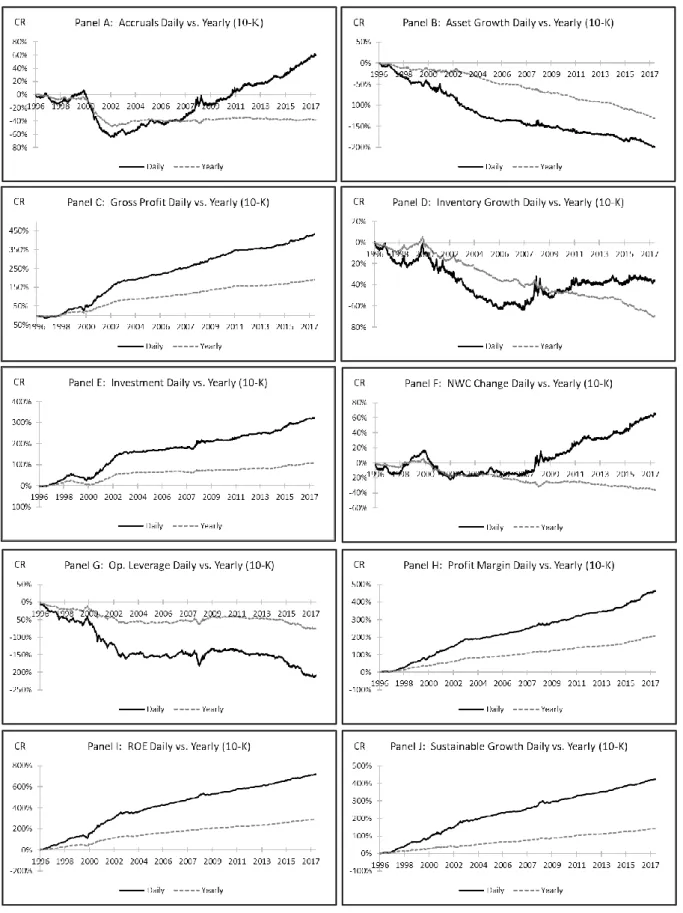
Figure II: Both the daily and yearly updating combo portfolios cumulated returns (CR) are

graphed throughout the years. Figure III, in the appendix, presents the same concept but for each individual anomaly. The over performance of the daily portfolio can be clearly seen.

Continuing with Table IX, the individual profitability anomalies perform as expected, with strong annual returns and almost no negative returns except for a few years. An interesting observation about these variables, and which connects to the previous discussion on the overdependence on shorting stocks, can be had: some of the robust profitability variable returns are clearly due to particularly years of economic crisis which significantly push the overall average return up, with ROE, for example, having a 145.7% spread during the year 2000, with this return most likely coming from shorting poorly performing stocks. The difficulties of actually achieving these shorts, in real life, in these specific circumstances of economic crisis, should be self explanatory.

Out of the 10 anomalies, only 5 are significant, based on p-value, for the 10-K section, while only 4 are significant for the 10-Q. This may seem a poorer result, when compared to the previous tables, however, these p-values are computed using the year to year standard deviation, and so only the strongest of differentials are deemed significant. When it comes to direct return comparison, 8 out of the 10 anomalies, for the 10-K section, have positive average return differentials, with 7 of these being larger than 5%, and 7 out of 10 have the same results for the 10-Q.

Table X, in the appendix, utilizes this daily minus yearly portfolio to present a five Fama-French regression on this portfolio’s daily returns, for both the 10-K and the 10-Q sections, with it also accounting for the risk-free rate of return. The idea being to better examine whether rebalancing daily versus yearly does still lead to an “alpha” creation, when an explanatory model is used,

21 and, to see, if some of these returns are correlated to, or explained, by these five Fama-French factors.

As for the results, for the 10-K section, an impressive 8 out 10 anomalies have a positive “alpha” (the exceptions, as expected, being asset growth and operating leverage), with the profitability anomalies creating the most. The average “alpha” is around 0.02%, for all anomalies, and 0.05% for the profitability anomalies. For the 10-Q section, 6 out of 10 anomalies create an “alpha” with the ones creating the most being, similarly, profitability anomalies, and with investment and inventory growth now creating negative “alpha”. These profitability anomalies show most positive correlation to the RMW (robust minus weak, an operating profit factor) as is to be expected, but are still sufficiently strong to consistently create strong positive “alpha”, even with this explanatory factor.

Overall, and as a closing remark to this examination of the different portfolio rebalance strategies section, it appears fair to say that, firstly, the daily portfolio performs generally better than all other typical forms of portfolio rebalancing, and that this is generally consistent throughout the period. Furthermore, the other rebalancing intervals, besides the daily one, fail to reliably outperform the yearly one and, therefore, should not be used. When transaction costs are accounted for, most of the extraordinary abnormal returns, from daily rebalancing, become insignificant when compared to the yearly one, except when using anomaly factors that relate to profitability. However, these profitability factors are also overly dependent on their short components which raises concerns as to their implementability. It seems that a daily portfolio rebalance strategy can only signify a better abnormal return performance when the investors is confident in the robustness of its anomaly strategy and its implementability.

4.2 Empirical Results – Event Study

The following sections now pertains to the results for the event time study discussed previously in the methodology, and in the introduction, and focuses no longer on investment strategies, as these contained numerous other stocks in the portfolios and did not focus solely on those having information releases, which makes them not as adequate for studying explanatory relationships in anomaly returns in a theoretical manner.

By examining more closely the relationship between abnormal returns and information release, again specifically for 10-K and 10-Q, the expectation is to see a stronger average return closer

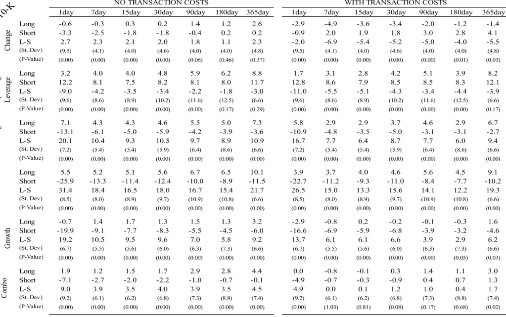
22 to the news release dates so as to imply that the market is updating to this new anomaly information and that, therefore, information, by itself, is primarily driving the anomaly returns. If these returns are not significantly present nearer to a news day, say when compared to the following 365 calendar days, then that is somewhat direct evidence against this explanation. The anomalies used are the exact same 10 as before and are also computed in the same way. A combo portfolio is also, once again, present. Here, however, the construction of the portfolios is quite different but simple in its approach: a stock that upon a financial statement release immediately warrants entry into a long or short portfolio, by being in the top or bottom decile for a specific factor, is lined up in an event type study with point zero being the news release. All stocks that fit this criteria, throughout 1996 to 2017 are then merged, so as to compute average returns for the first, second, third, and so forth days until a calendar year has passed (reducing period and firm specific effects to a minimum). Also, it is important to assert that these portfolios studied here are not replicable in real life, as investment portfolios (and this section has no interest in this aspect) as they are not fixed at a specific point in time but, instead, aggregate data from a 20 year period. Similar portfolios could, theoretically, be built but they would be severely undiversified and high on standard deviation and transaction costs (since they could only contain the few stocks that had financial statement releases on that day). Table XI and XII, in the appendix, present the overall results for this event time study. The left side of these tables presents data for 10-K statements and the right side 10-Q. The first table contains the first five anomalies and the second one contains the five remaining and the combo portfolio. Returns are presented in annualized absolute percentages for each of the anomalies and their respective long and short “legs”, as well as for the final “L-S”, long minus short, anomaly portfolio. These returns are averages of the daily returns up to the X days in the header row of the table. Standard deviation, on the other hand, represents the volatility within those X days holding periods. Finally, the p-value presented is in significance versus the 365 days annualized return (so as to properly test the null hypothesis that near news release returns are not significantly different from those farther from it).

Firstly, an overall look at the results. If the combo portfolio is taken, by itself, then it appears that the 10-K section establishes a clear relationship between proximity to news release and abnormal returns, with annualized returns up to 7 days all being strongly statistically significant versus the 365 day period (p-values are all below 0.01). Return spread, in annualized terms, for the 1 day, for example, versus the 365 days is 14.9% while, for the 7 days, it is 5.8%. This outperformance, however, is only present for both the short and long components, for the 1 day

23 returns. The 10-Q section, on the other hand, also has significant returns up to the 7 day mark, with a 1 day spread of 3.6%, however, these are also much weaker than for the 10-K. Other periods, above the 7 day mark, do not show significant differences from the 365 day return. From these, we can, for now, say that the first 7 days after a news information release, have a great impact in abnormal returns, with the news day itself, the 1 day mark, having more significance than the other 6 days. This corroborates the theory of a connection between information release and abnormal returns, in particular, the one with a quickly reacting market. This goes, somewhat, against the results by Bowles et al. (2018), whose methodology when calculating abnormal is slightly different but, nonetheless, relevant. In this paper, they find, similarly to our results, a statically significant abnormal return for the first days following a news release. However, this significance, for them, goes until the first 120 days, which supports a theory of slower to update market portfolios. A result also contrary to Bowles et al. (2018) is that they find non-news days to be equally important, in the first 30 days period, as the news day themselves. This is not necessarily the case for our results. For the 10-Q, this is somewhat true as the spread between 1 day and 7 days is merely 0.1%, and for the 1 day to 30 days it is 2.5%. However, for the 10-K section, we can clearly establish a significant difference with the news day returning 9.1% more annualized returns than the 7 days and 16.9% more than the 30 days.

As for the individual anomalies by themselves, we find that, in general, for the 10-K section, 7 out of the 10 anomalies have annualized returns, up to the first 7 days after a news release, which significantly differ from the annualized returns for the remainder of the year, with 5 of these also having a significant positive return difference. For the 10-Q, these numbers are 6 and 5 respectively. If we look only at the news day itself, these numbers increase to 9 and 6, for the 10-K, and 7 and 5, for the 10-Q. Considering that the 10-Q section is purposefully delayed, as to avoid look-ahead bias, more importance should be given to the 10-K section, which shows a clear significance for the days following a news release, even when looking at individual anomalies.

Once again, for both the 10-K and 10-Q, the anomalies related to profitability are the most important and consistent drivers for the overall combo portfolio’s strong positive returns near the news day (although they are not the only ones with, for example, accruals returning 45.4% on the averaged news days for 10-K). In fact, out of the 4 profitability factors (gross profit, profit margin, return on equity and sustainable growth) only gross profit and profit margin fail

24 to not be performing consistently better, up to the 7 days point, over the remainder 365 days. Regardless of this, when the significance exists, the spread in returns ends up being quite large (for example, sustainable growth has a 50% annualized return difference on the news day versus the 365 days, for the 10-K section). These results corroborate the over performance for these variables we have seen in the rebalancing investment strategies. Strong results, for these variables, were found also found by Engelberg et al (2017), who related the idea of biased cash flows expectations (which are contained within the profitability factors) being corrected on news arrival as the driver for returns and the general academic studied robustness. It seems this research somewhat validates this idea. Bowles et al. (2018) also, similarly, has significant results for these profitability anomalies.

As for other anomalies, asset growth continues to perform the poorest in the news day, albeit with a clearly stronger effect nearer to news days. Interestingly, net working capital change, operating leverage and accruals perform particularly well, with returns of 45.8%, 45% and 45.4%, for the 10-K section, but this performance only happens on the news day itself, contrarily to profitability factors, with returns quickly averaging down with time, which potentially explains why their performance was not seen in the rebalancing portfolio strategies.

Figure V: Cumulative returns (CR) are presented for the combo portfolio for both 10-K and

10-Q sections. With the long, short and the long-short portfolio returns discriminated. Point zero represents the day of a financial statement release (10-K or 10-Q) for a stock that warrants being included in the anomaly portfolio and then returns are accumulated for the following 240 trading days (approximately equal to 365 calendar days). Figure VI and VII, in the appendix, present the same but for each individual anomaly portfolios.

For the combo portfolios, evidence seems to suggest that there is no significant form of return clustering around the periods closer to a news release (as the evolution is quite linear). However,

25 these portfolios are also quite dependent on the profitability anomalies, which have this same characteristic.

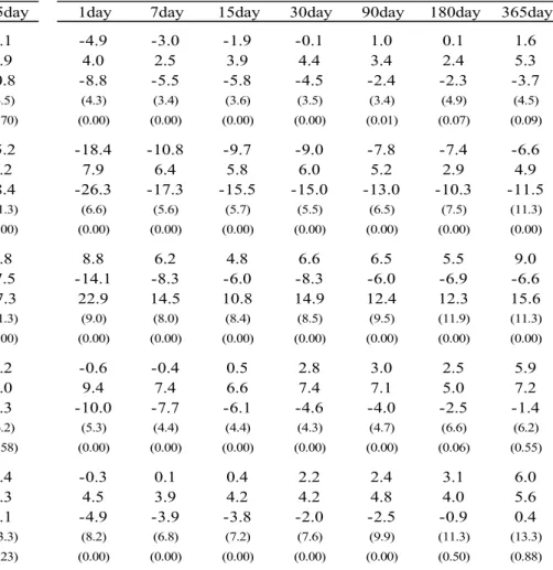
Table XIII further improves the comparability of the event time study by splitting the average annualized returns into calendar time intervals, specifically between 1 to 7 days, 7 to 15, 15 to 30, 30 to 90 and 90 to 365 days. This means each period is independent of each other and the returns are only averaged within the specific period, which makes comparisons between the different periods easier and less influenced by a particular strong result in either one.

Since news days themselves are now included within the 1 to 7 days period, they are not directly comparable. However, we feel, as discussed before, that their significance has already been established. Looking at the 10-K data, we find the combo portfolio not to be significant for the 1 to 7 and 7 to 15 periods. However, this is only due to the averaged return, coincidentally, being near the 90 to 365 one as, for the 1 to 7 days period, all 10 anomalies are deemed significantly different from the longer period, with 5 having a strong positive difference between them. As for the anomalies in the 10-Q section, these points generally remains true, but with more consistency than the 10-K section. The 1-7 combo portfolio is significant, and so are 7 out of the 10 anomalies for this period, with 6 of these having a solid return spread versus the 90-365 period. The first 3 time periods are also, generally, more significant than it was the case for the 10-K section.

Overall, there is a clear loss of significance as the days go by. It is, also, very rare, for the 90-365 period to ever improve on the anomaly returns by more than what had already been had from previous periods. That is to say that there is a never a consistent case for average annualized anomaly returns improving as they move to farther away, from news release, periods. This points to an idea of clustering of abnormal returns around the release of information.

However, reaching definitive conclusions is also difficult, as it appears that there is a great deal of volatility with return strength around the first 3 presented periods (for example, gross profit, on the 10-K section, has 24.1% returns for the first 7 days after a news release, which is then reduced to a 8.9% return for the 7-15 period and, then, a 25.6% return for the 15-30 period). It, generally, looks as if there is a large degree of market overreaction and correction, for these early periods, that eventually sets on a trend which continues for the remainder of the year. Largely, yes, periods closer to a news release do often create more abnormal returns than normal (potentially due to the discussed market over response to this news release) but it is also true