Mestrado em Biologia da Conservação
Dissertação
Évora, 2018
Esta dissertação inclui as críticas e as sugestões feitas pelo júri
Does habitat reachability affect the distribution of a
range expanding species in a fragmented landscape?
Cláudio Damásio João
Orientação: António Paulo Pereira de Mira
Pedro Alexandre Marques da Silva Salgueiro
Maria do Carmo Matos da Silva Salgueiro
ESCOLA DE CIÊNCIAS E TECNOLOGIA
ESCOLA DE CIÊNCIAS E TECNOLOGIA
DEPARTAMENTO DE BIOLOGIA
Does habitat reachability affect the distribution of
a range expanding species in a fragmented
landscape?
Cláudio Damásio João
Orientação:
António Paulo Pereira de Mira
Pedro Alexandre Marques da Silva Salgueiro
Maria do Carmo Matos da Silva Salgueiro
Mestrado em Biologia da Conservação
Dissertação
Évora, 2018
AGRADECIMENTOS
Primeiramente, queria agradecer aos meus pais não só pelo financiamento do meu percurso académico mas também por todo o apoio e suporte fornecido ao longo da minha vida.
Um especial agradecimento ao Pedro Salgueiro, à Carmo Silva e ao professor António Mira pela orientação e apoio para realização deste trabalho. Obrigado por todo o conhecimento que me transmitiram e pela vossa grande paciência para me explicar o maravilhoso mundo da estatística e do R que tinha passado despercebido perante os meus olhos.
Finalmente devo agradecer a todos os meus amigos que me acompanharam durante todo este percurso académico, por todas as palmadinhas nas costas que me deram, por todas as noites de trabalho intensivo passadas em conjunto e por todos os memoráveis momentos passados em conjunto que me ajudaram a moldar a pessoa que sou hoje.
Esta dissertação foi realizada no âmbito do projeto “ESTUDO E VALORIZAÇÃO DA BIODIVERSIDADE – COMPONENTE DA FAUNA - DAS FÁBRICAS MACEIRA-LIZ E CIBRA-PATAIAS, 2ª FASE”, pelo que agradeço à SECIL, Companhia Geral de Cal e Cimento, S.A., por todo o apoio disponibilizado a nível logístico e de cedência dos dados.
ÍNDICE
RESUMO ... 4
ABSTRACT ... 5
ENQUADRAMENTO ... 6
Fragmentação da paisagem e conetividade ... 6
Espécie alvo ... 9
INTRODUCTION ... 11
MATERIALS AND METHODS ... 14
Study area ... 14
Target species ... 15
Feeding and drey counts: ... 16
Environmental data ... 17
DATA ANALYSIS ... 20
Habitat suitability model - HSM ... 20
Permeability models ... 21
Model comparison ... 23
RESULTS ... 25
Habitat Suitability Model - HSM ... 25
Permeability models ... 26
Model comparison ... 29
DISCUSSION ... 32
Why to consider reachability in HSM? ... 32
Important factors describing red squirrel habitat selection and dispersion... 33
Caveats and future prospects ... 36
Contribute to conservation ... 37
CONSIDERAÇÕES FINAIS ... 39
2 ÍNDICE DE TABELAS
Tab I-Environmental data gathered and their respective landscape and patch ranges considered in this study. ... 19 Tab II-Variables incorporated in the final HSM, with the respective coefficient (β), confidence interval at 95% (C), relative importance value(RVI) and their significant p values (Sig:*<0.05;**<0.01;***<0.001) for each variable. ... 25 Tab III-Variables selected in the final permeability models with the total numer of dispersion areas considered in each dispersion distance and the respective proportion of presence/absence dispersion areas , and the respective coefficient (β), confidence interval at 95% (C), the relative importance value(RVI) and their significant p values (Sig:*<0.05;**<0.01;***<0.001), for each variable... 28 Tab IV-Variables incorporated in the final HSM+P, with the respective coefficient (β), confidence interval at 95% (C), relative importance value (RVI) and their significant p values (Sig:*<0.05;**<0.01;***<0.001) for each variable ... 30 Tab V-Variables incorporated in the final HSM and HSM+P, with the respective Akaike information criterion (AIC), the area under the curve of the receiver operating characteristic (AUC) and the threshold with the respective percentage of correct predictions for each model. ... 30
3 ÍNDICE DE FIGURAS
Fig. 1-Map of the study area with the respective land uses in Pataias and its location in Portugal (inset). Each sampled patch is marked with a dot: black dots indicate species presence, and grey dots indicate where species is absent. ... 15 Fig. 2- Simplified scheme for the modeling procedure used in the in this study. ... 24 Fig. 3-HSM and HSM+P prediction maps made using the environmental data: (A) Habitat suitability model; (B) HSM+P_1000; (C) HSM+P_1500; (D) HSM+P_2000. ... 31
4
Será que a acessibilidade de um habitat afeta a distribuição de uma
espécie em expansão numa paisagem fragmentada
?RESUMO
A fragmentação da paisagem pode influenciar a capacidade de espécies em expansão de alcançarem habitat adequado ao impedir os seus movimentos de dispersão. Para estimar este efeito, avaliamos a acessibilidade de habitat para o esquilo-vermelho numa paisagem fragmentada utilizando modelos espacialmente explícitos. Prevemos que o esquilo não ocupe todas as parcelas de elevada qualidade e que a ocupação não é só mediada pela qualidade do habitat mas também pela sua acessibilidade . Para testar estas hipóteses comparámos um modelo de adequabilidade de habitat (HSM) baseado unicamente em variáveis ambientais, com outros HSM que integravam a permeabilidade da paisagem para diferentes distâncias máximas de dispersão (1000, 1500, 2000 metros). Observamos que o HSM que integra a permeabilidade de habitat com uma capacidade de dispersão até 1000m apresenta melhor ajustamento aos dados observados. Os nossos resultados apontam que a acessibilidade do habitat influência a distribuição do esquilo vermelho.
5
Does habitat reachability affect the distribution of a range
expanding species in a fragmented landscape?
ABSTRACT
Landscape fragmentation may influence the ability of range expanding species to reach suitable habitat by impeding its dispersal movements. We used a spatially explicit modeling approach to access the influence of habitat reachability on the distribution of the red squirrel in a fragmented landscape. We hypothesize that the red squirrel does not occupy all suitable habitat patches, and patch occupancy is not only mediated by habitat suitability but also by its reachability. To test these hypothesis we compared a habitat suitability model (HSM) based only on environmental data to other three HSMs considering landscape permeability at different maximum dispersal distances (1000, 1500, 2000 meters). Our results show that the model that took in consideration a 1000m dispersal distance was better fitted to observed occupancy data. Our findings show that habitat reachability influences the distribution of red squirrel, since suitable habitat patches may not be reachable.
6
ENQUADRAMENTO
Fragmentação da paisagem e conetividade
A fragmentação de habitat e a introdução de barreiras que diminuem a conetividade da paisagem podem afetar o movimento dos indivíduos e, consequentemente a sua dispersão para novas áreas (Andersson & Bodin, 2009; Gibbs et al., 2010; Haddad et al., 2015; Merrick & Koprowski, 2017). A conetividade da paisagem pode ser descrita como a capacidade desta para promover ou dificultar o movimento de indivíduos (e fluxo genético), desempenhando um papel vital na distribuição de espécies (Uezu et al., 2005). Assim a conservação e restauro da conetividade é essencial à manutenção de populações viáveis e à conservação da biodiversidade em geral (Chardon et al., 2003; Merrick & Koprowski, 2017).
A alteração do uso do solo devido à crescente humanização das paisagens causa fortes impactos na biodiversidade. A subdivisão de um habitat originalmente contínuo em parcelas de menores dimensões origina uma área onde as parcelas de habitat nativo se encontram separadas por uma matriz mais ou menos inóspita, e onde o movimento dos indivíduos é reduzido, dando origem a uma paisagem fragmentada (Fletcher et al., 2018; Haddad et al., 2015). Nestas paisagens, efeitos como a perda de habitat, o aumento do efeito de orla e o isolamento de parcelas e populações tornam-se mais prevalentes e, consequentemente as populações que nelas permanecem ficam mais suscetíveis a fenómenos de competição, erosão genética (Pardini et al., 2018; Verbeylen et al., 2003), e a fenómenos de estocasticidade demográfica e ambiental, reduzindo a sua viabilidade a longo prazo (Pereira & Jordán, 2017). A introdução de barreiras ao movimento também contribui para um aumento do isolamento (Andersson & Bodin,
7 2009; Haddad et al., 2015; Verbeylen et al., 2003), limitando a dispersão de indivíduos para novos habitats (Gibbs et al., 2010; Wauters et al., 2010). Segundo Ronce (2007) a dispersão é um processo fundamental para o movimento de genes numa paisagem e por, isso é um aspeto crítico para garantir a persistência global da espécie em caso de extinção local. A sua limitação poderá causar uma disrupção da dinâmica populacional a longo prazo e levar as populações à extinção local (Wauters et al., 2010).
Durante a dispersão, os indivíduos iniciam um processo de seleção de território de acordo com as suas preferências de habitat (Sánchez-Clavijo et al., 2016). Este processo não é aleatório, fatores como a qualidade de habitat, risco de predação, competição inter e intraespecífica e os custos de dispersão associados são considerados durante este processo (Gurnell et al., 2002; Morris, 2003; Sánchez-Clavijo et al., 2016). O elevado risco de predação e de exploração de novas áreas tem elevados custos para o fitness do indivíduo, podendo levar à ocupação de parcelas com menor qualidade em detrimento de assumir o risco de se deslocar a grandes distâncias em busca de melhores habitat (Morris, 2003; Sánchez-Clavijo et al., 2016). Este efeito torna-se mais prevalente em indivíduos com grande mobilidade que habitam em paisagens fragmentadas altamente heterogéneas (Sánchez-Clavijo et al., 2016).
Durante o processo de dispersão, os indivíduos procuram por indícios relativos à qualidade do habitat, normalmente procurando características semelhantes do o seu habitat natal, podendo levar a uma maior tendência para um indivíduo se dispersar para parcelas adjacentes com estes atributos (Richard & Armstrong, 2010; Sánchez-Clavijo et al., 2016; Verbeylen et al., 2009). Contudo, as parcelas podem não fornecer indícios fidedignos que verdadeiramente reflitam a qualidade de habitat. Os elevados custos de
8 fitness associados à dispersão em paisagens fragmentadas juntamente com indícios de qualidade de habitat falaciosos, podem levar indivíduos a ocupar parcelas subótimas, mas acessíveis (Richard & Armstrong, 2010; Sánchez-Clavijo et al., 2016; Xu et al., 2018; Verbeylen et al., 2003), não alcançando parcelas com maior qualidade de habitat.
Assegurar uma boa capacidade de movimento para as espécies alvo, ou seja, conservar uma elevada conetividade da paisagem é fundamental para debelar estes efeitos sobre as populações (Chardon et al., 2003). Entender como a conetividade da paisagem (Merrick & Koprowski, 2017) influencia a dispersão e de seleção de habitat é um aspeto crítico para o desenvolvimento de métodos mais precisos para identificar áreas críticas para aplicar esforços de conservação.
Neste estudo iremos analisar os fatores que influenciam a distribuição de uma espécie em expansão numa paisagem fragmentada utilizando modelos baseados na presença ou ausência da espécie para avaliar o papel da acessibilidade das parcelas no processo de seleção do habitat. Para tal foi selecionado o esquilo-vermelho (Sciurus vulgaris, Lineus 1758). Esta espécie constitui um bom modelo para este estudo devido à sua elevada capacidade de dispersão e à sua recente expansão na área de estudo. Definimos duas hipóteses: (1) o esquilo-vermelho não ocupa todas as parcelas de elevada qualidade e, (2) a ocupação de parcelas não é só mediada pela qualidade do habitat mas também pela sua acessibilidade.
Para tentar responder a esta hipótese, comparamos a área potencial de ocupação do esquilo-vermelho obtida por modelação da adequabilidade de habitat (Habitat Suitability Model-HSM), unicamente baseado em características das parcelas que são relevantes para a presença do esquilo, e três modelos de adequabilidade de
9 habitat, que têm em consideração a permeabilidade da paisagem para o esquilo (HSM+P). Os modelos de permeabilidade basearam-se na simulação de possíveis rotas de dispersão aleatórias que o esquilo pode tomar entre as parcelas, utilizando o método de Brownian bridges (Codling et al., 2008).
Espécie alvo
O esquilo-vermelho é um pequeno mamífero arbóreo, diurno e com grande capacidade de dispersão que ocorre naturalmente na região Paleártica. Esta espécie era bastante comum até ao século XVI quando foram declarados extintos em Portugal. Isto deveu-se à constante pressão demográfica causada pela desflorestação de grandes áreas florestais para a construção naval e para criação de áreas agrícolas. No século XX foram implementadas novas políticas florestais que promoveram a reflorestação de grandes superfícies de pinhal em Portugal, levando ao reaparecimento do esquilo na década de 80 no norte do país. Atualmente é possível encontrar esquilo-vermelho no Norte e Centro de Portugal e em algumas regiões a sul de Lisboa (Ferreira et al., 2001; Mathias & Gurnell, 1998; Rocha et al., 2017, 2014; Vieira et al., 2015).
Em termos de habitat, prefere zonas de coníferas e bosques mistos onde existe grande quantidade de alimento ao longo do ano e árvores suficientemente grandes para a construção ninhos ou tocas. São animais bastante plásticos capazes de habitar parques perto de zonas urbanas. (e. g. Haigh et al., 2017; Lurz et al., 2005). Alimentam-se principalmente de sementes e frutos de coníferas, árvores decíduas e de arbustos. Quando estes alimentos são escassos a sua alimentação pode incluir fungos, flores, insetos, ovos, líquenes e, em casos extremos, casca de árvore (Lurz et al., 2005; Moller,
10 1983). Quando se alimenta de sementes de coníferas, nomeadamente de pinheiro-bravo (Pinus pinaster Aitom) e pinheiro-manso (Pinus pinea L.), deixa marcas facilmente identificáveis nas pinhas (Bang & Dahlstrøm, 2001), indícios normalmente usados em metodologias de censo de esquilo-vermelho (Gurnell et al., 2004).
Neste estudo foram inicialmente testadas diferentes metodologias para a deteção do esquilo, de forma a aferir a viabilidade da sua aplicação. Neste âmbito foram testadas as seguintes metodologias: 1) máquinas fotográficas de disparo automático com recurso a diferentes iscos, 2) transetos com pontos para a observação direta de indivíduos e 3) transetos para a deteção de indícios de presença. Dos três métodos testados apenas com o último se obtiveram resultados fiáveis, tendo sido este escolhido para avaliar a presença de esquilo em cada parcela. Este método apresenta a vantagem de ser mais expedito, podendo investir-se num maior número de locais amostrados, e melhorando a eficácia na obtenção de dados para responder aos nossos objetivos.
11
Does habitat reachability affect the distribution of a range
expanding species in a fragmented landscape?
INTRODUCTION
Landscape connectivity, which is the process by which landscape characteristics promote or impede individual movement (Taylor et al., 1993), can play a vital role in species prevalence as it provides suitable routes for species dispersal and expansion (Merrick & Koprowski, 2017; Ronce, 2007).
The process of habitat fragmentation begins with the transformation of native habitats in a landscape, forming a matrix of native patches separated by human-transformed habitats (Haddad et al., 2015). With increasing humanization of habitats, several pitfalls become more prevalent such as the depletion of resources, intensification of edge effects and isolation of patches and populations (Pardini, et al. 2018). Populations trapped in isolated patches become susceptible to deterministic processes (Pardini et al., 2018). These will make populations more susceptible to increased competition for resources, genetic eroding as a result of inbreeding, and demographic and environmental stochastic processes threatening their long-term persistence (Pereira & Jordán, 2017; Verbeylen et al., 2003). Thus maintaining high connectivity between patches is indispensable for maintaining healthy and viable populations (Chardon et al., 2003).
The land use changes and introduction of barriers that disturb landscape connectivity influence both species daily movement and capability of dispersion (Andersson & Bodin, 2009; Haddad et al., 2015), hindering its dissemination into new
12 habitats (Gibbs et al., 2010; Merrick & Koprowski, 2017; Verbeylen et al., 2003). According to Ronce (2007), dispersal can be defined as the movement of individuals with potential consequences for gene flow across space. During this process, each individual begins accessing new available habitats when searching for a new territory, linking species behavior with species distribution (Sánchez-Clavijo et al., 2016). The selection of a new patch to establish is not random. Factors such as habitat quality, predation risk, interspecific/intraspecific competition (Gurnell et al., 2002) and dispersion costs are considered and guide individual choices during the selection (Morris, 2003; Sánchez-Clavijo et al., 2016). Moreover, the elevated risk of predation and high energy cost of foraging large and distant areas will affect individual fitness (Morris, 2003). Some individuals might prefer to occupy less suitable patches than risking to reach distant higher quality patches (Sánchez-Clavijo et al., 2016). This is particularly relevant in heterogeneous landscapes, where animals do not have enough information about unexplored patches, thus searching for cues to infer about its suitability such as habitat structure and reliable food sources. Most cues are believed to follow general habitat requirements usually found in their natal home ranges (Sánchez-Clavijo et al., 2016; Wauters et al., 2010), which may bias dispersal movements into adjacent habitats (Richard & Armstrong, 2010). However, those cues might not give reliable information about the quality of the habitat (Patten & Kelly, 2010; Sánchez-Clavijo et al., 2016), masking potentially poor habitats. Therefore the high dispersion costs and misleading cues associated with heterogeneous fragmented landscapes may lead individuals to occupy sub-optimal (Xu et al., 2018), but reachable, patches rather than higher quality habitat patches that are far away. Understanding the drivers of dispersion and habitat selection may provide insights on the specific needs and constraints for each species to
13 move inside the landscape (i.e., functional landscape connectivity Merrick & Koprowski, 2017; Verbeylen et al., 2003), allowing the identification of critical areas where conservation efforts should be concentrated.
In this study, we aim to determine the factors that influence the distribution of a range expanding species in a highly fragmented landscape and to unveil the role of patch reachability on its distribution. We used a presence/absence modeling approach to access landscape connectivity for a species with a known high dispersal ability that recently occupied the study area in central Portugal.
To achieve our objectives, we will use data on the distribution of the Eurasian red squirrel (Sciurus vulgaris Linnaeus. 1758). This species is a suitable model to this study due to its high dispersal ability and recent expansion. We hypothesize that (1) the red squirrel does not occupy all suitable habitat patches, and (2) patch occupancy is not only mediated by habitat suitability but also by its reachability.
We compared the potential area of occupation of the Eurasian red squirrel estimated by a habitat suitability model (HSM) based only on environmental data to the area predicted by three other HSM incorporating landscape permeability. We build landscape permeability models by simulating possible movement routes between patches truncated at different maximum dispersal distances (1000m, 1500m, 2000m). We used the Brownian bridges method to simulate random connections between patches (Codling et al., 2008) in order to compute the permeability models.
14
MATERIALS AND METHODS
Study area
(Rivas-Martínez et al., 2011).
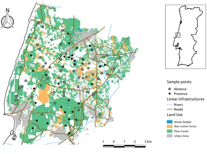
The study was carried out in Pataias (39º37´04´´N 9º01´02´´W), Leiria, Central Portugal (Fig.1), as part of the project “Study and valuation of biodiversity – Fauna componente – at Maceira-Liz and CIBRA-Pataias plants” in 2011. The study area has a total of 11 121ha and is mainly dominated by a standard production forest matrix comprised by the following land uses: Pine forest (44%, Pinus pinaster Aitom and Pinus pinea L.), orchards (17%), urban areas (9%) non-native plantations (6%, Eucalyptus globulus Labill, Acacia longifolia Wild and Acacia dealbata Link). Other land uses known to be important for squirrel, such as oak forests (Cagnin et al., 2000), were vestigial (<1%) and not considered for the study design.
The pine forests and the non-native forests in the study area are subjected to an intensive management similar to the Faustmann rotation model (Rosa et al., 2018). Each patch is subjected to a high disturbance cycle with three distinct phases: clear-cut patches are converted in to newly planted forests subjected to frequent thinning and grown to adult plantations (with different ages depending of the species). This creates an heterogeneous mosaic landscape with well-defined patches with different age and understory cover and structure (Rosa et al., 2018; Salgueiro et al., 2018).
The orography is mainly flat, with a mean altitude of 70 m a.s.l., with a predominance of sandy soils forming sandy dunes (Instituto do Ambiente, 2003). The climate is Mediterranean, with some Atlantic influence, characterized by hot summers and tempered winters (Rivas-Martínez et al., 2011; Monteiro-Henriques et al., 2016).
15
Fig. 1-Map of the study area with the respective land uses in Pataias and its location in Portugal (inset). Each sampled patch is marked with a dot: black dots indicate species presence, and grey dots indicate where species is absent.
Target species
We targeted the Eurasian red squirrel (Sciurus vulgaris L. 1758) as a model species to test our hypothesis due to its high dispersal mobility and the peculiar history in Portugal. This species was common before the 16th century when they became extinct due to heavy habitat loss, mostly from logging (Ferreira et al., 2001; Mathias & Gurnell, 1998; Rocha et al., 2014). New reforestation policies involving the plantation of large pine areas in the 20th century enabled the reappearance of the squirrel from the North
16 of Portugal in the 80´s (Santos-Reis & Mathias, 1996). Nowadays the squirrel can be found throughout the North and Central regions of Portugal and in some areas south of Lisbon where it was introduced (Ferreira et al., 2001; Rocha et al., 2017, 2014). This indicates that the species is currently expanding its range on the Portuguese territory and may have not yet occupied all the suitable habitat.
Feeding and drey counts:
We carried out pedestrian transects to identify squirrels feeding presence signs and dreys in each sampled patch. This method offers a rather efficient way to sample large areas due to its expeditious nature, making it ideal for studies concerning the distribution of squirrel within the landscape and access the connectivity between patches (Ferreira et al., 2001; Gurnell et al., 2004).
Each transect consisted in 100m linear paths in which signs were prospected. We standardized transect length at 100m to investigate the effect of smaller patches in red squirrel occurrence. Signs were prospected 20m around the transect, giving special attention to the base of older trees with high pine cone production, generally an attractive feature to red squirrels (e.g., Cagnin et al., 2000; Moller, 1983). We considered the species to be present whenever a drey or an eaten pine cone with the squirrel specific strip pattern was found during the transect (Bang & Dahlstrøm, 2001; Gurnell et al., 2004). Otherwise, if no signs were found we considered it as an absence. To minimize false positives, we only considered fresh signs of squirrel presence.
17 A total of 89 transects was performed. All the transects were at least 300m apart from each other to ensure data independency (Cagnin et al., 2000). Two replicates were made in 2011, one in spring between April and July, and other in autumn between October and December.
Environmental data
All environmental data was gathered by performing spatial analysis through geographical information systems. We produced a land use map of the area (Fig.1) using Bing Maps aerial photography (year: 2011; resolution: 30 cm), and the delimitation and classification of each patch was validated in the field using a GPS device (Garmin eTrex20).
Most of the environmental variables were extracted using a moving window approach with two buffer distances: 150m and 500m. We used a 150m radius buffer to represent the mean home range of the squirrel in similar habitats (e.g., Cagnin et al., 2000; Lurz et al., 2005) and 500m to represent the mean maximum home range observed in regions with higher latitudes (e.g., Andrén & Delin, 1994; Lurz et al., 2005).
We extracted habitat composition by calculating the area of each land use within the two buffer distances. Due to method constraints (transects were only performed on pine forest patches) we only considered two land uses for habitat suitability modelling, adult pine plantations (AdultPine) and young pine plantations (YoungPine). For other non-prospected land uses such as urban areas (towns and quarries) and non-native plantations we calculated the shortest distance from the transect to the nearest patch.
18 We also estimated the total coverage of shrub area by considering the mere presence of shrubs (above 0.30m) on the patch (variable Shrubs). Additionally, we defined three classes to disentangle the effects of shrub height: 1) areas with short (<0.30m) or no shrubs (NoShrubs); 2) areas with shrub height between 0,3 and 1m (MediumShrub); and 3) areas with shrub height above 1m (TallShrub).
We assessed landscape fragmentation for each sampled transect buffer by calculating edge (high contrast edges - edges between adult pine plantations and farmland/bare soil areas; low contrast edges- edges between adult pine plantations and young pine plantations or young pine plantations and farmland/bare soil areas; and total edge), patch size metrics (patch size and mean patch size); and landscape mosaic metrics (number of habitats, patch density, Shannon diversity index and aggregation index). We also measured the Euclidean distances to other landscape features, such as linear infrastructures (roads) and water bodies (rivers and lakes).
All variables (Tab I) were extracted using the program QGIS 2.18 (QGIS Development team, 2016) and Fragstats (McGarigal, et al. 2012).
19
Variable category
Acronym Variable description Units Study area Range
Sampled patch Range Landscape
fragmentation
dist2lce Distance to low contrast edges m [0;1468] [14.14;601.1]
dist2hce Distance to high contrast edges m [0;1033] [22.36;591.4]
lce500 Total length of low contrast edges
within 500m
m [0:108200] [0;97000]
lce150 Total length of low contrast edges
within 150m
m [0;17000] [0;10100]
hce500 Total length of high contrast
edges within 500m
m [0;74700] [0;60100]
hce150 Total length of high contrast
edges within 150m
m [0:18300] [0;9500]
dist2edge Distance to edges m [0;1033] [14.14;320]
te500 Total length of edges within 500m m [0;150600] [5200;126700]
te150 Total length of edges within 150m m [0;23300] [0;16200]
ai150 Aggregation index within 150m [74.04;100] [89.97;100]
shdi150 Shannon's diversity index within
150m
[0;1.94] [0;1.31]
pd150 Patch density within 150m [44.44;711.1] [44.44;355.6]
patchsize Area of each patch ha [0.01;383.6] [0.72;383.6]
nhabitat500 Number of habitats within 500m [1;9] [1;6]
nhabitat150 Number of habitats within 150m [1;9] [2;9]
mps500 Mean patch size within 500m ha [1780;37910] [407;32621]
mps150 Mean patch size within 150m ha [93;38364] [34;38360]
dist2water Distance to water bodies m [0;4200] [120;3730]
Land use AdultPine500 Adult pine forest area within 500m ha [0;792100] [76900;786800]
AdultPine150 Adult pine forest area within 150m ha [0;72900] [0;72900]
YoungPine500 Young pine plantations area
within 500m
ha [0;738300] [0;672300]
YoungPine150 Young pine plantations area
within 150m
ha [0;72900] [0;72900]
dist2urban Distance to urban areas m [0;1887] [64.0;1690]
UrbanArea150 Urban area within 150m ha [0,72900] [0;10600]
UrbanArea500 Urban area within 500m ha [0;584900] [0,210900]
dist2road Distance to roads m [0;1818] [22.36;1748]
dist2NonNative Distance to Non Native areas m [0;1728] [20;1024]
NonNative150 Non native plantations area within
150m
ha [0,72900] [0,29800]
NonNative500 Non native plantations area within
500m
ha [0;580200] [0;235400]
Shrub coverage NoShrubs150 Shrubless patch area within 150m ha [0;72900] [0;72900]
dist2shrub Distance to shrub areas 8 (m) m [0;1130] [31.62;874.6]
NoShrubs500 Shrubless patch area within 500m ha [0;792100] [3400;776200]
TallShrub150 Tall shrub patch area within 150m ha [0;72900] [0;72900]
TallShrub500 Tall shrub patch area within 500m ha [0;4240] [0;364900]
Shrubs150 Shrubed area within 150m ha [0,72900] [0,72900]
Shrub500 Shrubed area within 500m ha [0;792100] [15900;788700]
MedShrub150 Medium shrub patch area within
150m
ha [0;792100] [15900;792100]
MedShrub500 Medium shrub patch area within
500m
ha [0;792100] [15900;744900]
20
DATA ANALYSIS
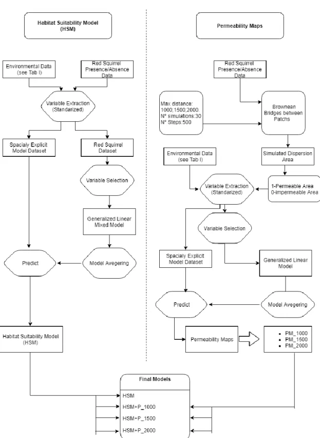
For this study we divided the data analysis in two sections, 1) we built a habitat suitability model (HSM) only considering the environmental data and 2) three habitat suitability models considering the landscape permeability (HSM+P), by simulating Brownian bridges between each sampling point. All the data analyses processes and modeling were done with R 3.4.4 (R Core Team 2018). A scheme of the model creation process can be found in Fig.2.
Habitat suitability model - HSM
All the extracted environmental variables were standardized. Extracted variables were selected after checking for outliers, normality, collinearity and homogeneity. All variables that did not met the requirements were transformed (square root and logarithmic transformations) (Zuur et al., 2010, 2009), or discarded. The remaining variables were used to create a mixed effect model based on the package lme4 (Bates et. al., 2018). Presence/absence of squirrels in each transect was accounted as the response variable and the season in which the survey was carried out (spring and autumn) as the random factor (Zuur et al., 2009). The model obtained was subjected to a model dredging process using the package “MuMin” (Bartoń 2018). Model selection was based on Akaike’s Information Criterion corrected for small samples (AICc). A model averaging approach was performed by weighting a set of competitive models (in our case, a 95% confidence interval on the cumulative sum of Akaike weights) to estimate the magnitude of the effects of the environmental variables on the response variable
21 (Pita et al., 2009), allowing a comparable measure between them by estimating their relative importance (RVI). To avoid problems related to multicollinearity, some variables were excluded from the analysis to keep variance inflation factors below 2 for all variables (Zuur et al., 2010). Residuals were plotted to check for patterns to evaluate the model fitness.
We also measure the relevance of influential samples by calculating Cooks’s distance (R core team 2018). Spatial autocorrelation was measured by Moran’s I (“ape” package, Paradis et al., 2011) and Spatial auto correlograms (“ncf” package, Bjornstad, 2018). The HSM was transposed to a spatially explicit model using the variables calculated for all the studied landscape.
Permeability models
The permeability models were based on the variables present on simulated random dispersion areas between each pair of patches. Each simulated dispersion area was created using Brownian bridges (adehabitatLT, Calenge, 2006) which allows to create random walks for a dispersing individual with a minimal amount of information input. This way we incorporated in our models the random nature of animal movement during dispersal instead of a predetermined path. Each simulated path consisted on 500 steps between each pair of patches, simulated 30 times. By stacking the 30 simulated paths we created an area where dispersion events between each pair may occur. Both the number of steps and the number of simulations were previously tested to check for effects on the size of the area of dispersion. Since further increase of the number of both parameters showed no effect, we choose to use the above-mentioned values. For each
22 area of dispersion between each pair of patches we extracted the standardized mean values of the environmental variables.
Dispersal distances for this species are referred to be many times longer than the daily movements carried out within the home range area (Gurnell et al. 2002), with larger dispersal distances for fragmented landscape (Wauters et al., 2010). For this purpose we tested several distances ranging two, three and four times the maximum distance of the home range considered in this study (500m radius), i.e. we considered as maximum distance of dispersal 1000m, 1500m and 2000m for the simulated areas of dispersion.
The simulated areas of dispersion connecting two patches where squirrels were present were considered permeable and simulated areas of dispersion connecting patches where the squirrel was present in one and absent in the other were considered impermeable.
The variable selection procedure for the landscape permeability models was similar to the methodology used in the HSM. An independent generalized linear model was built for each maximum dispersal distance. The response variable was the dichotomous classification of permeable / impermeable coded as presence / absence data.
The models obtained were subjected to a dredging process using the package “MuMin” (Bartoń, 2018) and a model averaging procedure was performed considering all models within a 95% confidence interval of the Akaike weights. All selected variables had a VIF<2. The final landscape permeability models were then used to make three Habitat Suitability Models that account for landscape permeability (HSM+P), one for
23 each dispersal distance considered: P_1000, P_1500 and P_2000. Each HSM+P was created by adding the model predictions of each permeability map to the initial HSM model as a new independent variable and rerunning these models. Each model was checked again to avoid multicollinearity (VIF<2) between the newly added variable and the initial set of variables in the HSM (Fox &Weisberg, 2011).
Model comparison
We compared the three new HSM+P models with the initial HSM. The four models were compared using both Akaike information criterion (AIC) and the area under the curve (AUC) of the receiver operating characteristic (ROC) using the package “AUC” (Ballings & Van den Poel 2013). A map was created for each model for a better visualization of the results (Fig.3).
In addition, we compare the performance of each HSM and HSM+P models by calculating the percentage of correct classifications (presence/ absence). In each model we calculated different threshold values by selecting the one that maximizes a higher percentage of correct predictions (Liu et al., 2005; Manel et al., 2001).
24
25
RESULTS
Habitat Suitability Model - HSM
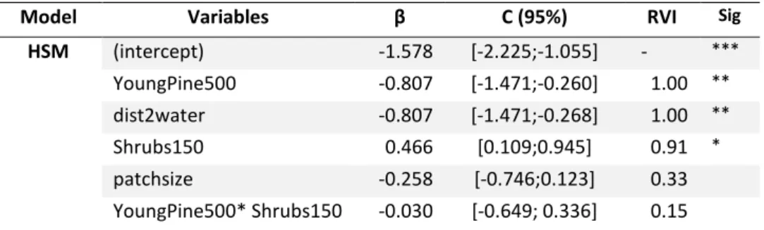
The habitat suitability model comprised five variables, from which the most important were: young pine plantation area (YoungPine500: coef=-0.807, RVI=1.0), distance to water (Dist2water: coef=-0.895, RVI=1) and areas with shrub cover (Shrub150: coef=0.466, RVI=0.91) (Tab II). The red squirrel avoided young pine plantations, preferred areas with the presence of shrubs (above 0.30m) and patches near water bodies (such as small ponds and rivers). We also detect an interaction effect between young pine plantation area and shrub cover (YoungPine500*Shrubs150: (coef=-0.30, RVI=0.15), meaning that although the species tended to avoid large young pine plantations, it can occur in small young pine plantations if the understory is dominated by shrubs. Patch size (coef=-0.258, RVI=0.31), showing a slight tendency for squirrel occurrence in smaller patches of habitat, i.e. in more fragmented areas.
Tab II-Variables incorporated in the final HSM, with the respective coefficient (β), confidence interval at 95% (C), relative importance value (RVI) and their significant p values (Sig:*<0.05;**<0.01;***<0.001) for each variable.
Model Variables β C (95%) RVI Sig
HSM (intercept) -1.578 [-2.225;-1.055] - *** YoungPine500 -0.807 [-1.471;-0.260] 1.00 ** dist2water -0.807 [-1.471;-0.268] 1.00 ** Shrubs150 0.466 [0.109;0.945] 0.91 * patchsize -0.258 [-0.746;0.123] 0.33 YoungPine500* Shrubs150 -0.030 [-0.649; 0.336] 0.15
26 Permeability models
A total of three permeability models were created according to the three different dispersal distances considered (P_1000), 1500m (P_1500); and 2000m (P_2000). Some variables were found to be consistent between models, although each model resulted on different predictions due to the different sample size (P_1000: 83 dispersion areas; P_1500: 213 dispersion areas; and P_2000: 349 dispersion areas; see Tab III for details on presence/absence ratio).
For instance, distance to water (Dist2water-PM_1000: coef= -0.004; P_1500: coef= -0.002; P_2000: coef= -0.002) and young pine plantation area (YoungPine500-P_1000: coef= -0.001; P_1500: coef= -0.001; P_2000: coef= -4.54E-4) were the most important variables in all the permeability models with an RVI>0.8. In both cases the coefficient had a negative influence, meaning that patches near water increase landscape permeability, while young pine plantation patches can act as a barrier to the dispersal of the squirrel. Patches with shrub cover (Shrub500 - P_2000: coef= 3.94E-4; TallShrub500 - P_1000: coef= 0.049; P_1500: coef= 0.001) also had a major importance in all permeability models (most RVI>0.8), assuming a positive trend, i.e., the presence of shrub cover improves landscape permeability.
In all models, non-native plantations tend to show a negative effect (Non-native500-P_1000: coef= -0.042, RVI =0.41; P_1500: coef= -0.055, RVI=1.0; P_2000: coef= -0.210, RVI=0.7), which implies that this land use also acts as a barrier to the dispersal of the red squirrel. However, in some cases, this relation has an equivocal meaning since the confidence intervals include a zero value (for example at P_1000).
27 Urban areas had a different effect in each dispersal distances, but in some cases with equivocal meaning. While it may affect habitat permeability negatively at medium distances (UrbanArea500-P_1500 coef= -0.010, RVI= 0.29), at longer distances they appear to have positive effect (P_2000, coef= 0.199, RVI= 0.8).
Variables describing habitat fragmentation show some ambiguous (and sometimes equivocal) effects from model to model. Edge effects show some opposite trends: while high contrast edges (HCE500-P_1000: coef= 0.000, P_1500: coef= 0.000,) had a positive influence at lower dispersal distances (1000m and 1500m), total edge (P_2000: coef= -0.001) had a negative influence at higher distances (2000m). Distance to road (dist2road-P_1000: coef= -0.001, RVI= 0.25; P_2000: coef= -0.001) had a negative coefficient, which shows that it may provide dispersal routes for the squirrel. Nonetheless, these variables had a lower relative importance in the models, showing an RVI below or equal to 0.4.
28
Tab III-Variables selected in the final permeability models with the total number of dispersion areass considered in each dispersion distance and the respective proportion of presence/absence dispersion areas , and the respective coefficient (β), confidence interval at 95% (C), the relative importance value(RVI) and their significant p values (Sig:*<0.05;**<0.01;***<0.001), for each variable.
Dispersion areas
Total Absence Presence β Confidence
(95%) RVI P PM_1000 88 53 35 (intercept) 2.335 [-0.973;5.642] YoungPine500 -0.001 [ -0.002;-0.001] 0.98 * Dist2water -0.004 [-0.007;-0.002] 1.00 ** TallShrub500 0.049 [0.007;0.091] 0.87 * NonNative500 -0.042 [-0.112;0.0272] 0.41 Shrubs500 0.000 [-0.000; 0.001] 0.41 dist2road -0.001 [-0.003;0.001] 0.28 hce500 0.000 [-0.006; 0.006] 0.25 PM_1500 213 135 78 (intercept) 2.391 [1.116;3.666] *** NonNative500 -0.055 [-0.097;-0.013] 1.00 * YoungPine500 -0.001 [-0.001;-0.001] 1.00 *** Dist2water -0.002 [-0.004;-0.001] 1.00 *** TallShrub500 0.001 [0.000;0.001] 1.00 *** UrbanArea500 -0.010 [-0.041;0.022] 0.29 Hce500 0.000 [-0.003;0.003] 0.26 PM_2000 349 237 112 (intercept) 0.291 [-1.848; 2.430] NonNative500(sqrt) -0.25 [-0.506; 0.007] 0.70 . YoungPine500 -0.000 [ -0.001;-0.000] 0.83 * UrbanArea500 (sqrt) 0.199 [ 0.016;0.382] 0.80 * Dist2water -0.002 [-0.003;-0.001] 1 *** Shrubs500 0.000 [0.000;0.001] 1 ** te500 -0.000 [-0.002;0.001] 0.42 Dist2road -0.001 [ -0.002;0.000] 0.41
29 Model comparison
Of all the four models compared, the HSM+P with the permeability model of 1000m (HSM+P_1000) has shown a better fit and performance (AIC=172.4, AUC=0.829) than the rest of the models (HSM: AIC=175.08, AUC=0.815; HSM+P_1500: AIC=177.05, AUC=0.814; HSM+P_2000: AIC=176.54, AUC=0.814). Even though having a higher complexity compared with the original HSM (one less degree of freedom, see Tab V for more information), the AIC difference between both models is higher than 2. A higher number of correct predictions can also be observed in HSM+P_1000 (table V), which further validates our previous statement(Liu et al., 2005; Manel et al., 2001).
The HSM+P1000m has an added value when compared with the HSM based only on environmental data, meaning that there is a higher probability for squirrel to occur in patches in highly permeable areas that are within 1000m in the surroundings of the occupied patches (P_1000: coef= 0.4507, confidence [0.041;0.907]). Furthermore, habitat permeability showed a high relative importance in the model (RVI=0.79), contrasting with the other RVI values obtained for the habitat permeability at 1500m and 2000m (0.12 and 0.24, respectively) (Tab II & Tab IV) found in the other models (HSM+P1500 and HSM+P2000). At these distances the permeability models are less suited and more equivocal in estimating red squirrel occurrence (P_1500: coef= 0.04141, confidence= [-0.410;0.480]; P_2000: coef= -0.1757, confidence= [-0.665;0.286]).
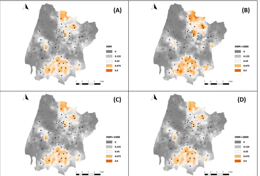
In Fig.3 we show the prediction maps (i.e. the occurrence probabilities of red squirrel for the whole study area) derived from each of the four developed HSM models. Although the prediction maps are very similar, identifying the same suitable areas, the HSM+P1000 tends to show higher probabilities of occurrence in areas where the squirrel
30 is present when compared with the HSM, showing a better fit of the model. For this reason, this model also shows a higher threshold, correctly predicting 82% of our data (Tab V).
Tab IV-Variables incorporated in the final HSM+P, with the respective coefficient (β), confidence interval at 95% (C), relative importance value (RVI) and their significant p values (Sig:*<0.05;**<0.01;***<0.001) for each variable
Model Variables β C (95%) RVI Sig
HSM+ P_1000 (intercept) -1.632 [-2.269;-1.074] - *** dist2water -0.854 [-1.542;-0.270] 1.00 ** YoungPine500 -0.768 [-1.392;-0.214] 1.00 * Shrubs150 0.424 [-4.00E-04;0.861] 0.65 . Patchsize -0.259 [-0.717;0.173] 0.17 YoungPine500* Shrubs150 -0.167 [-0.674;0.302] 0.03 * P_1000 0.451 [0.041;0.907] 0.79 HSM+ P_1500 (intercept) -1.603 [-2.229;-1.058] - *** dist2water -0.823 [-1.494;-0.263] 1.00 ** YoungPine500 -0.819 [-1.489;-0.236] 1.00 ** Shrubs150 0.519 [0.109;0.944] 0.89 * Patchsize -0.307 [-0.761;0.123] 0.31 YoungPine500* Shrubs150 -0.139 [-0.647;0.334] 0.13 P_1500 0.041 [-0.410;0.480] 0.12 HSM+ P_2000 (intercept) -1.598 [-2.218;-1.055] - *** dist2water -0.772 [-1.427;-0.225] 1.00 * YoungPine500 -0.903 [-1.587;-0.304] 1.00 ** Shrubs150 0.508 [0.094;0.936] 0.89 * Patchsize -0.252 [-0.717;0.197] 0.25 YoungPine500* Shrubs150 -0.144 [-0.668;0.342] 0.11 P_2000 -0.176 [-0.665;0.286] 0.24
Tab V-Variables incorporated in the final HSM and HSM+P, with the respective Akaike information criterion (AIC), the area under the curve of the receiver operating characteristic (AUC) and the threshold with the respective percentage of correct predictions for each model.
Model AIC AUC Threshold %correct
HSM 175.08 0.815 0.37 0.75
HSM+P_1000 172.40 0.829 0.39 0.82
HSM+P_1500 177.05 0.814 0.36 0.808
31
Fig. 3-HSM and HSM+P prediction maps made using the landscape variables: (A) Habitat suitability model; (B) HSM+P_1000; (C) HSM+P_1500; (D) HSM+P_2000.
32
DISCUSSION
Why to consider reachability in HSM?
Our results show that in fragmented landscapes optimal habitat are not fully occupied by range expanding species, as we predicted in our first hypothesis. Instead, they tend to occupy habitats with higher reachability. While testing three permeability models with different dispersion distances, we showed that HSM can be improved by including this information, thus validating our second hypothesis.
The HSM+P considering the 1000m dispersion range showed a better fit with better AIC and AUC values than the original HSM and the other HSM+P with different dispersion ranges. A higher cut-off threshold and percentage of correct predictions could also be found in HSM+P1000, meaning that the improved model has better performance and precision that any other. This means that the red squirrel in our study area is likely to disperse a maximum of 1000m from its natal breeding area. Interestingly, increasing dispersion distance in permeability models resulted on a gradual decrease of the overall fitness of HSM+P. This can be explained by the movement behavior of the squirrel, some studies based on telemetry support that this species can move up to 1000m when dispersing in fragmented landscapes (Lurz et al., 2005; Verbeylen et al., 2009; Wauters et al., 2010). Our conclusions are in accordance with these authors’ results.
Furthermore, the inclusion of permeability in habitat suitability models improve the fitenssof these models . Therefore, these models are better suited to disentangle
33 the different factors that permit or obstruct the dispersion of the target species and identify possible barriers in a landscape.
Important factors describing red squirrel habitat selection and dispersion
Most of the variables retained in the models are shared between the landscape permeability models and the HSM based only on environmental data, suggesting (as expected) that patches with suitable habitat requirements offer the least amount of resistance to dispersion (Richard & Armstrong, 2010; Wauters et al., 2010). Variables related with the general requirements of the squirrel such as food and cover availability (e.g. presence of adult pine forests, shrubs and the proximity to water bodies) share high importance values across all models and are in accordance with the feeding and foraging habits of the squirrel (Lurz et al., 2005; Moller, 1983).
It is conceivable that HSM models are more rigid while identifying the habitat and resource requirements of the red squirrel than permeability models. Nonetheless, areas lacking such requirements (non-suitable habitat areas) can still offer low resistance to movement (Andrén & Delin, 1994; Delin & Andrén, 1999, Keeley et al., 2016).
Surprisingly, distance to water revealed an important variable for red squirrel occurrence. Our results show that red squirrel tended to occupied areas near water. Although this relation has not been described in most studies relating red squirrel, Lurz (2010) refer that this relation may occur, possibly associated to specific conditions. Our study area is under Mediterranean influence, resulting in hot summers. In addition, the
34 dominant soil is mostly sandy, thus highly permeable. The combination of these conditions results on very dry summers, where water availability may be a limiting factor. The preference of red squirrels for near water territories may be a response to prevent such harsh periods.
Young pine plantations were one of the most relevant variable selected, showing a negative effect on red squirrel occurrence. Young pine plantations have a low pine cone production and a reduced canopy, being densely packed and subjected to regular trimming disturbance cycles. This intensive management hinders the growth of a shrub understory, further reducing the food and cover availability in these patches (Rosa et al., 2018), and consecutively reducing the suitability of this habitat for squirrel occurrence or movement (Cagnin et al., 2000; Gurnell et al., 2002; Lurz et al., 2005).
Shrub cover also had an important role determining the occurrence of the squirrel and landscape permeability. The red squirrel preferred patches where the understory was composed by a shrub layer, avoiding areas without cover. Shrubs can provide secondary food resources and refuge when moving on the ground (e.g. Lurz et al., 2005; Moller, 1983). Nonetheless, we found some differences between HSM and permeability models. Unlike the HSM where we only detected the presence of shrub to be important, the maximum height category (higher than 1m) was more relevant in permeability models. This preference might be related with the use of shrubs as stepping stones to cross patches where tree canopy does not form a continuous matrix (Teixeira et al., 2017).
Habitat fragmentation had a low relative importance value in the models and assumed equivocal relations to red squirrel occurrence. Most of the habitat
35 fragmentation variables identified in the models referred to patch size and edge effect, which tend to increase with increasing fragmentation. According to our results, Red squirrel tended to occur in highly fragmented areas, with lower patch size and higher edge length. Much of the suitable habitat locates in clusters of small patches alternating with lower quality habitats. The high movement ability of the squirrel may facilitate its dispersion by overcoming small patches of lower habitat quality (Cagnin et al., 2000; Delin & Andrén, 1999; Fey et al., 2016; Haigh et al., 2017; Wauters et al., 2010).
Non-native plantations had negative influence in the permeability models, possibly constituting barriers to squirrel dispersion. Some studies prove that other small rodents might use these patches as a foraging landscape or as corridors (Teixeira et al., 2017). However, in our case, the presence of non-native plantations may decrease the availability of food resources and limit the necessary cover for shelter (Lurz et al., 2005; Moller, 1983). Moreover, these land uses are also subjected to an intensive management (nine to ten-year cycles), which have an impact on canopy cover and understory.
The urban areas had an ambiguous effect on the permeability models according to the dispersal distance used to calculate them. At shorter dispersal distances, urban areas had a negative impact on the dispersion; however, a positive effect was observed at distances until 2000m, meaning that at higher dispersal distances the urban areas may be permeable. This result may be a consequence of using unsuited dispersal distances for this study area. As referred above, the 1000m dispersal distance was better adjusted, which agreed with other authors (Lurz et al., 2005; Wauters et al., 2010). In
36 our case, considering higher dispersal distances could result on unreal movement dispersion areas, biasing the variable effects.
Caveats and future prospects
Predicting animal distribution in a fragmented landscape with limited data on their movement ecology can be a challenging task. Habitat suitability models often not include connectivity related variables (e.g. Chardon et al., 2003; Uezu et al., 2005; Verbeylen et al., 2003). As our study shows, the inclusion of these metrics may prove essential to estimate correctly the distribution of a species in a fragmented landscape. However, the lack of information regarding animal movement (telemetry data)
hampers the addition of such metrics. Here we propose an alternative to estimate habitat permeability using simple occurrence data.
In this study, we tested HSM with three landscape permeability models calculated from three different maximum dispersal distances. The use of Brownian bridges in this approach allowed to simulate different random dispersion areas in contrast to the standard Euclidean lines between nodes (Poniatowski et al., 2016; Richard & Armstrong, 2010). Other methods are available to infer the probability of movement between patches, such as the least cost path modeling. However, this method depends on previous HSM models to build a resistance surface (Keeley et al., 2016). In addition, only one path is considered as a possible path between patches, which may not truly reflect the randomness of an animal movement.
37 We believe that our approach constitutes a suitable method to include landscape permeability in habitat modeling, allowing to overcome some shortfalls, such as the lack of movement data. Nonetheless, in the future, telemetry data may be a relevant resource to validate our findings.
Contribute to conservation
The creation of more informative models will allow to improve landscape management and enable more accurate predictions of future impacts of land use changes (Andersson & Bodin, 2009; Drake et al., 2017; Gurnell et al., 2002; Verbeylen et al., 2003). Our approach allowed the development of more precise models to predict occupied habitats and assess possible dispersion barriers for range expanding species while accounting for the movement ability of a species to reach suitable habitat patches.
The comparison between HSM and HSM+P can serve as a diagnosis tool to identify unreachable habitats and areas with greater resistance to dispersion. The identification and creation of small corridors with a complex matrix of shrubs between unreachable and occupied patches would facilitate the dispersion of the squirrel to suitable habitats. In addition, while identifying areas more susceptible to isolation, this methodology can serve as a basis to assess possible impacts in the distribution of populations, due to changes in management schemes, plantation of non-native species, or construction of new infrastructures (Verbeylen et al., 2003). In fact, this method can give important clues for mitigation measures aiming to avoid or minimize possible impacts on species population and distribution.
39
CONSIDERAÇÕES FINAIS
Prever a distribuição de populações em paisagens fragmentadas pode ser uma tarefa difícil. A inclusão da conetividade da paisagem em modelos de adequabilidade de habitat pode ser essencial para estimar corretamente a distribuição de populações. Contudo, a inexistência de dados relativos ao movimento dos animais, como por exemplo dados de telemetria, dificulta a inclusão desta informação nos modelos (Chardon et al., 2003; Uezu et al., 2005; Verbeylen et al., 2003). Neste estudo pretendemos desenvolver uma alternativa para estimar a permeabilidade do habitat utilizando apenas dados de ocorrência de espécie. O uso de Brownian bridges para simular o movimento aleatório de animais entre parcelas ocupadas e não ocupadas permite o desenvolvimento de modelos que incluam a permeabilidade do habitat.
Os nossos resultados apontam para que a distribuição do esquilo-vermelho em paisagens fragmentadas é também mediada pela acessibilidade das parcelas. Este facto contribui para a existência de constrangimentos na distribuição da espécie, não ocupando todo o habitat favorável disponível. Os modelos de adequabilidade de habitat para espécies em expansão podem, então, ser melhorados com a incorporação da permeabilidade da paisagem.
No nosso caso, a incorporação da permeabilidade da paisagem para os movimentos do esquilo, considerando uma capacidade de dispersão de até 1000m nos modelos de adequabilidade de habitat, melhorou significativamente o ajustamento do modelo. Este resultado comprova que a acessibilidade das parcelas influencia a distribuição das populações em paisagens fragmentadas. Ademais, a acessibilidade das parcelas está intimamente ligada à capacidade de dispersão dos indivíduos, uma vez que
40 o modelo de permeabilidade selecionado reflete aquela que é a distância de dispersão para esta espécie como referenciado em vários estudos (Lurz et al., 2005; Verbeylen et al., 2009; Wauters et al., 2010). Isto implica que há uma maior probabilidade de as parcelas de habitat adequado serem ocupadas se estiverem a uma distância máxima de 1000m de outra parcela ocupada e que a matriz entre estas não oferece resistência.
A inclusão da permeabilidade da paisagem permite identificar parcelas de habitat adequado inacessíveis envolvidas por uma matriz inóspita à dispersão de indivíduos. A identificação destas áreas pode ser útil para a implementação de medidas de conservação de forma a promover a conetividade entre parcelas de habitat adequado. Paralelamente, permite também identificar áreas vulneráveis a impactos decorrentes da alteração de usos do solo ou da construção de infraestruturas (Andersson & Bodin, 2009; Drake et al., 2017; Gurnell et al., 2002; Verbeylen et al., 2003).
A nossa abordagem parece constituir um método viável para incluir a permeabilidade do habitat em modelos de adequabilidade de habitat, permitindo a construção de modelos mais informativos para a conservação de espécies e mitigação de impactos.
41
REFERÊNCIAS
Andersson, E., & Bodin, Ö. (2009). Practical tool for landscape planning? An empirical investigation of network based models of habitat fragmentation. Ecography, 32(1), 123–132. https://doi.org/10.1111/j.1600-0587.2008.05435.x.
Andrén, H., & Delin, A. (1994). Habitat Selection in the Eurasian Red Squirrel , Sciurus vulgaris , in Relation to Forest Fragmentation relation to forest fragmentation. Oikos, 70, 43–48. https://doi.org/10.2307/3545697.
Bang, P., & Dahlstrøm, P. (2001). Animal Tracks and Signs. Ney York: Oxford University press.
Cagnin, M., Aloise, G., Fiore, F., Oriolo, V., & Wauters, L. A. (2000). Habitat use and population density of the red squirrel, sciurus vulgaris meridionalis, in the sila grande mountain range (Calabria, South Italy). Italian Journal of Zoology, 67(1), 81– 87. https://doi.org/10.1080/11250000009356299.
Chardon, J. P., Adriaensen, F., & Matthysen, E. (2003). Incorporating landscape elements into a connectivity measure: a case study for the Speckled wood butterfly (Pararge aegeria L.). Landscape Ecology, 18, 561–573.
Codling, E. A., Plank, M. J., & Benhamou, S. (2008). Random walk models in biology.
Journal of The Royal Society Interface, 5, 813–834.
https://doi.org/10.1098/rsif.2008.0014.
Delin, A., & Andrén, H. (1999). Effects of habitat fragmentation on Eurasian red squirrel ( Sciurus vulgaris ) in a forest landscape. Landscape Ecology, 14, 67–72.
Drake, J. C., Griffis-Kyle, K. L., & McIntyre, N. E. (2017). Graph theory as an invasive species management tool: case study in the Sonoran Desert. Landscape Ecology, 32(8), 1739–1752. https://doi.org/10.1007/s10980-017-0539-2.
Ferreira, A. F., Guerreiro, M., Álvares, F., & Petrucci-Fonseca, F. (2001). Distribución y aspectos ecológicos de Sciurus vulgaris en Portugal. Galemys, 13, 155–170.
Fey, K., Hämäläinen, S., & Selonen, V. (2016). Roads are no barrier for dispersing red squirrels in an urban environment. Behavioral Ecology, 27(3), 741–747. https://doi.org/10.1093/beheco/arv215.
Fletcher, R. J., Didham, R. K., Banks-Leite, C., Barlow, J., Ewers, R. M., Rosindell, J., Haddad, N. M. (2018). Is habitat fragmentation good for biodiversity?. Biological Conservation, 226, 9–15. https://doi.org/10.1016/j.biocon.2018.07.022.
Gibbs, M., Saastamoinen, M., Coulon, A., & Stevens, V. M. (2010). Organisms on the move: ecology and evolution of dispersal. Biology Letters, 6, 146–148. https://doi.org/10.1098/rsbl.2009.0820
Gurnell, J., Clark, M. J., P, W. W. L., Shirley, M. D. F., & Rushton, S. P. (2002). Conserving red squirrels (Sciurus vulgaris): mapping and forecasting habitat suitability using a Geographic Information Systems Approach. Biological Conservation, 105(1), 53–64.
42 Gurnell, J., Lurz, P. W. W., Shirley, M. D. F., Cartmel, S., Garson, P. J., Magris, L., & Steele, J. (2004). Monitoring red squirrels Sciurus vulgaris and grey squirrels Sciurus carolinensis in Britain. Mammal Review, 34, 51–74. https://doi.org/10.1046/j.0305-1838.2003.00028.x
Haddad, N. M., Brudvig, L. A., Clobert, J., Davies, K. F., Gonzalez, A., Holt, R. D., Townshend, J. R. (2015). Habitat fragmentation and its lasting impact on Earth ’ s ecosystems. Applied Ecology, 1, 1–9. https://doi.org/10.1126/sciadv.1500052 Haigh, A., Butler, F., O’Riordan, R., & Palme, R. (2017). Managed parks as a refuge for
the threatened red squirrel (Sciurus vulgaris) in light of human disturbance. Biological Conservation, 211, 29–36. https://doi.org/10.1016/j.biocon.2017.05.008 Liu, C., Berry, P. M., Dawson, T. P., & Pearson, R. G. (2005). Selecting thresholds of
occurrence in the prediction of species distributions. Ecography, 28, 385–393. Lurz, P. W. W., Gurnell, J., & Magris, L. (2005). Sciurus vulgaris. American Society of
Mammalogists, 769, 1–10.
https://doi.org/10.1644/1545-1410(2005)769[0001:SV]2.0.CO;2
Manel, S., Williams, H. C., & Ormerod, S. J. (2001). Evaluating presence – absence models in ecology : the need to account for prevalence. Journal of Applied Ecology, 38, 921–931.
Mathias, M. da L., & Gurnell, J. (1998). Status and Conservation of the Red squirrel (Sciurus vulgaris) in Portugal. Hystrix, 10, 13–19.
Merrick, M. J., & Koprowski, J. L. (2017). Circuit theory to estimate natal dispersal routes and functional landscape connectivity for an endangered small mammal. Landscape Ecology, 32(6), 1163–1179. https://doi.org/10.1007/s10980-017-0521-z
Moller, H. (1983). Foods and foraging behaviour of Red (Sciurus vulgaris) and Grey (Sciurus carolinensis) squirrels. Mammal Review, 13, 81–98.
Monteiro-Henriques T, Martins MJ, Cerdeira JO, Silva PC, Arsénio P, Silva Á, Bellu A, Costa JC 2016. Bioclimatological mapping tackling uncertainty propagation: application to mainland Portugal. International Journal of Climatology, 36(1): 400-411. doi:10.1002/joc.4357.
Morris, D. W. (2003). Toward an ecological synthesis: A case for habitat selection. Oecologia, 136(1), 1–13. https://doi.org/10.1007/s00442-003-1241-4
Pardini, R., Nichols, E., & Püttker, T. (2018). Biodiversity Response to Habitat Loss and Fragmentation. Reference Module in Earth Systems and Environmental Sciences, 0– 11. https://doi.org/10.1016/B978-0-12-409548-9.09824-9
Patten, M. A., & Kelly, J. F. (2010). Habitat selection and the perceptual trap. Ecological Applications, 20(8), 2148–2156. https://doi.org/10.1890/09-2370.1
Pereira, J., & Jordán, F. (2017). Multi-node selection of patches for protecting habitat connectivity: Fragmentation versus reachability. Ecological Indicators, 81, 192–200. https://doi.org/10.1016/j.ecolind.2017.06.002