Backtesting of an investment
strategy taking advantage of the
volatility in stock prices
Margarida Paixão
Dissertation written under the supervision of Joni Kokkonen
Dissertation submitted in partial fulfilment of requirements for the MSc in
Backtesting of an investment strategy taking advantage
of the volatility in stock prices
Margarida Paixão
Abstract
This thesis tests a strategy of Technical Analysis for the stock market which tries to catch profits from variations in stock prices (volatility) and does that by assuming that the price comes back to the mean most of the times. Therefore, the strategy sells when the price is above the mean by a certain distance and buys when it is below. The strategy was tested both on the S&P 500 index and for 30 separate companies of the US market. Intraday data of 5 minutes was used. The results for the S&P 500 are not very robust, however as expected, for separate companies the performance was better, having obtained statistically significant positive returns for the period. The risks of the strategy are associated with whether or not the stock exhibits the behavior that is expected consistently in time and more frequently than it exhibits undesired behaviors. For the period studied, the gains overcome the losses. Using a portfolio with a larger number of companies can help reduce risk.
Esta dissertação testa uma estratégia de Análise Técnica no mercado de acções. O objectivo é tentar obter lucro com as variações dos preços das acções (volatilidade), assumindo que o preço volta à média muitas vezes. Assim sendo, a estratégia vende se o preço estiver acima da média, e compra se estiver abaixo. Os testes foram aplicados ao índice S&P 500, tal como para 30 diferentes empresas no mercado americano. Os dados usados foram dados intradiários do preço das acções, com intervalos de 5 minutos. Os resultados dos testes com o S&P não se revelaram robustos, no entanto, como esperado, os resultados para empresas separadas foram bons, tendo obtido lucro significativo estatisticamente, para o período testado. Os riscos associados à estratégia passam pela dúvida de se as acções irão sempre exibir os comportamentos que a estratégia prevê, e se vão exibi-los mais frequentemente do que os comportamentos não previstos. Para o período estudado, os ganhos foram maiores que as perdas. Aumentando o número de empresas no portfólio o risco pode ser diminuído.
Acknowledgements
I would like to thank my thesis supervisor, Joni Kokkonen, for having made it possible that I executed this work and for the assistance given. I am also grateful to Fundação para a Ciência e a Tecnologia, for financial support.
Contents
Introduction... 1
Literature Review... 3
Data... 6
The Strategy Proposed... 7
Results... 11
Mean Strategy in the S&P 500... 11
Buy-Only Strategy in the S&P 500... 17
Mean Strategy for separate companies in the S&P500... 19
Conclusion... 26
Appendices... 29
Appendix A... 29
Appendix B... 30
List of Figures and Tables
Figures
Figure 1 - Diagram showing how the strategy procedure operates
Figure 2 - Alphabet stock (GOOGL) during some period on the 19th January 2018
Figure 3 - Cumulative returns of both the S&P 500 and the variations strategy and total
returns
Figure 4 - Returns from Buy and Sell parts of the strategy separately
Figure 5 - Cumulative returns of the variations strategy against the S&P 500 returns (a loss
limit of one standard deviation was applied to the strategy) and further characteristics
Figure 6 - Returns from Buy and Sell parts of the strategy separately (with a maximum loss
on the sell side equal to one standard deviation)
Figure 7 - Cumulative returns of the variations strategy against the S&P 500 returns (with a
loss limit of one standard deviation and a training window of 3 days) and further characteristics
Figure 8 - (1) Graph with Cumulative Returns; (2) further characteristics of the strategy and
the benchmark and (3) chart with the magnitude of the returns
Figure 9 - Performance of the variations strategy
Figure 10 - Distribution of returns of the 30 companies in the sample Figure 11 - Distribution of returns by sectors
Tables
Table 1 - Settings for the mean strategy executed on the S&P 500 data Table 2 - Results of buy and sell parts in the variations strategy
Table 3 - Results of buy and sell parts in the variations strategy Table 4 - Sensitivity Analysis Results
Table 5 - Settings for the buy-only strategy executed on the S&P 500 data Table 6 - Sensitivity Analysis Results
Table 7 - Settings for the mean strategy executed on separate companies' stocks
Table 8 - Results of the mean strategy for a group of 30 companies in the S&P 500. For each
company it is presented the return of the variations strategy, the returns of its separate parts: buy and sell, and the percentage of positive or zero returns that they make
Introduction
In this thesis, an investment strategy for the stock market is back-tested. The strategy takes advantage of brief variations in the stock prices, and it is built to make profits if these variations return to the mean consistently. It is one agreed factor by Academia that the returns of stock prices are random. However, posing some questions such as: "Do investors make their decisions to buy or sell the stocks based on information? Or do they do it based on how they feel about it?" or "Can people sell their shares in panic when they are loosing value?" can make us think about the way investments are being made, whether the agents in the market make rational decisions and based on information or not. I prefer to believe that there is a component of the process that generates the stock prices that is predictable, because it is generated by decisions of people who sometimes behave repeatedly. Of course in practice we would need incredibly clever tools or access to key information in order to identify exactly what effect the decisions of people influence the market, but it is possible that there are some trends in the stock prices being created by this predictable behavior.
The stock market in its microstructure is made in a way that gives investors the power to define the stock prices. Furthermore, the price changes a lot in short periods. It can happen that investors buy a stock for a price, and afterwards the price goes down, and they paid too much. Perhaps they do not look for nearby prices to decide if they are getting the best value when they buy the stock because they want the shares with urgency. In small intervals in which the stock price changes, there have not been significant changes to the company characteristics that justify the change in share price. Either the company is growing fast or there was some new information coming out, or, as it also happens, there is no change to value that justifies the volatility rather than subjective factors, rather than people imposing their opinion about the share value into the market price. Therefore, the microstructure of the market could allow for some market intermediate that sells and buys to other people and makes a profit. This could be possible given that the spreads are not too large, given that there is volatility and that the intermediate can predict what investors will want to do next: buy or sell shares. The way the strategy in this thesis is done is by having this type of "intermediate" that buys when the stock is at a lower price (perhaps a minimum) and then sells to the investors later when they want to buy, or the opposite when the stock is at a higher price. Perhaps then this intermediate would even reduce the volatility of the stock, by smoothing the
deviations. When the stock price drops he buys, so the stock price does not go as far low as it would go, and when the stock rises it would not go as far high.
If people themselves are predictable and repeat the same mistakes across time, then in general there could be some hypothetically predictable component in the market. It would be hypothetically predictable because the information needed to make conclusions is hardly available. Perhaps now with the introduction of technology, and new ways of monitoring, more information can be retrieved. Additionally, in some situations the "masses", i.e. all investors react in the same way, since they have similar psychological traits, for example with panic selling and such events, the price can generate a pattern because so many people are doing the same thing. Speculators making bets, investors who regret their decisions and then close their positions right away, agents investing without research and disagreeing with the market’s view of the stock, these are situations that could deviate the price of the stock from the fundamental value. Some investors might even trade for what they “feel” about a stock or based on what everyone else has been saying about it, which sometimes is not based on accurate information either. As long as the price of securities is decided by the laws of offer and demand and there are people on the other side making the trades, I do not believe that stock returns can be random, because people make mistakes, they are not efficient, and they repeat their mistakes.
Some technical analysis techniques already use complex measures to find patterns, mostly visual patterns, in the time series of stock prices. This thesis will not focus on these tools though, but will occupy with finding whether there are potential profits in a strategy that assumes that variations of stock prices are temporary deviations that will come back to the mean. The idea that some variations of stock prices deviate for a while but then return to the mean has already been discussed by the Literature and the phenomenon is given the name of 'mean reversion', even though this phenomenon is reported for longer periods, for example months or years whereas here the strategy takes advantage of really fast variations using intraday data. This thesis tests the strategy to understand if there are profits from this supposed phenomenon that the prices return to the mean. It is a strategy of Technical Analysis because we rely on past prices solely to evaluate the strategy and because it treats a visual pattern found in the series of stock prices. If the phenomenon happens more times than it does not happen, then the strategy proposed will yield positive returns. The volatility will also be used as an indicator in this strategy. The investment strategy will try to achieve positive returns with reduced risk, since it will aim at being right about the phenomenon most of the
times. The motivation for this strategy is also due to the fact that there are a lot of potential profits in the variations of the stock prices, which in total, make up much bigger returns than when we just choose a direction. If we would "stretch" the line drawn by the time series of prices, the variations in stock price make up a really big distance that could be taken advantage of. Furthermore, in this era of technology and given that there are already algorithms investing for institutions, rises the opportunity for investing in a very small time scale, where perhaps small differences in prices can originate profits, and emerges the opportunity of automating the strategies, which is very useful for some like the one created in this thesis, which handles intraday data.
In this thesis, tests of the strategy on the S&P 500 will be firstly executed. Then tests will be performed for 30 separate companies in the S&P, however I believe that the potential of this strategy will be maximized for the companies' stocks separately, since the S&P is an agglomerate of different stocks so the variations are not as large. I also expect the strategy to perform better for still moments, when there is no information coming out associated with that stock, though I will not test that.
Literature Review
Technical Analysis is the analysis of the price of a stock or the graph given by the price series of a stock in order to create investment strategies, not considering any other financial variables that could describe the company further. This is a topic that has generated distinct views across different parties in the Finance world. The Academia usually takes a negative position on it. They argue that Technical Analysis is not viable. Nonetheless, technical analysis indicators are used in real trade situations by investors, funds, and investment strategies are developed based on it.
Brock, Lakonishok and LeBaron (1992) published an article in the Journal of Finance where they test two technical analysis techniques: Moving Average-oscillator and trading range break-out. Inside these two techniques they also used several different variations of the sub-techniques and changed the parameters, in order to test these sub-techniques in some detail. They used data from the Dow Jones Industrial Average from 1897 to 1986. The moving average technique is performed by having two averages: one for a longer time period and another one
for a shorter period. The strategy buys when the short-term average goes above the long-term average, as this is a signal that an up-trend is starting; and sells when the short-term average is below the long-term average. The trading range break-out technique is based on buying after a local maximum and selling after a minimum. It is signaled by buying when the price is within the 'resistance level' or selling when it is within the 'support level'. Brock, Lakonishok and LeBaron (1992) found in their study some positive results defending these technical analysis techniques.
Bessembinder and Chan (1998) publish a paper refuting the results of Brock, Lakonishok and LeBaron (1992), arguing that the good results they had been obtained were due to errors from nonsynchronous trading.
Lo, Mamaysky and Wang (2000) made a study focusing on Technical Analysis and whether or not it was a field worth giving attention to. They said that Technical Analysis is not very well seen because the way Technical Analysts talk about the techniques is too elaborate for a field that sometimes seems a little subjective, and where the analyses can depend on the person who is identifying the trends. Therefore, they decided to use an objective method to identify popular technical patterns. By defining the technical rules in a systematic way through an algorithm, they made sure it was a computer (which is unbiased) identifying the patterns and not a person (who is biased). In order to remove noise in the time series they used smoothing estimators and then they ran the tests by executing kernel regressions. They found that some indicators provide valuable information.
Neftci (1991) made a study about Technical Analysis. He starts by saying that there is no reason why so much time is spent on Technical Analysis because no technique can outperform the Wiener-Kolmogorov prediction. Furthermore, he says that the statistical properties of Technical Analysis are unknown and the techniques are not well defined mathematically. However, he later states that the Wiener-Kolmogorov method is linear, which means that perhaps Technical Analysis can add value when it comes to predicting non-linear behavior. Moreover, there have been other studies that indicate that some characteristics of stock price movements are not linear. He gives the example of a bubble that ends in a crash. The crash itself cannot be described linearly. With the Wiener-Kolmogorov prediction one can only deal with up to the first and second moments, so Technical Analysis could come into play to fill this gap. Neftci (1991) tested three major classes of Technical Analysis techniques,
quantified them and formalized them. He focused on the Moving Average technique; particularly he tests a 150 days average. In the period of 1795 to 1910 the results were not significant, however for the period of 1911 to 1976 they were highly significant in confirming some predictive power of the technique. Neftci (1991) argues that the reason for it to start being significant in the later period might be because of people themselves believing that Technical Analysis has some value, which can indeed make it happen in a self-fulfilling way. Leigh, Purvis and Ragusa (2001) publish a paper in Decision Support Systems where they use techniques as pattern recognition, neural network and genetic programming in order to identify technical patterns. They show that there is potential coming from studies like this. In the Literature, there are doubts about which type of process generates the stock market's returns. It is hard to model these returns with one single process, thus what happens is different processes are used in different situations. The Black and Scholes model assumes a Brownian motion with a drift to model stock returns. And though it is not scientifically correct, as we now know, it still provides a very useful benchmark for the price of options. Some argued that the stock price exhibited the behavior of a random walk, which would have explained why it persists around its previous value, however, Lo and MacKinlay (1988) show that the stock market does not follow a random walk, not suggesting though any new process to describe stocks and also denying at the same time that the alternative of the stationary mean-reversing process could be possible. Other processes can model the mean of the returns and the volatility and different tools have been created to try to describe the stock returns, however with errors. The uniqueness of the stock prices series makes it difficult to find a constant process that could define it. The only agreeable fact in the Literature is that the S&P 500 tends to go up in the long run and that its returns exhibit a bigger number of occurrences around small positive returns than the respective Normal distribution would have. The Academia also agrees that the returns are random, i.e. that the stock is not more likely to go up than to go down and vice-versa.
Cowles and Jones (1937) made a study about sequences and reversals in the stock market. A sequence is a positive return following a positive return or a negative return following a negative return. A reversal is the opposite: a positive return following a negative return or vice-versa. They calculated the ratio of sequences to reversals and showed that there are more sequences than reversals in short and medium periods of time. From 20 minutes intervals to 3
years, all the data showed a higher number of sequences than reversals. This gives some support to Momentum strategies. The interval that Cowles and Jones (1937) showed to be the one with a higher ratio of sequences to reversals was 1 month (ratio of 1.66), which contrasts with the period of 12 months chosen by Jegadeesh and Titman (1993) for their Momentum strategy. From 4 years until 10 years intervals, the opposite occurs, i.e. reversals are more frequent than sequences, excepting for the 5 years interval where they are the same. Cowles and Jones (1937) verified the results with a probabilistic test to check if their findings could have been obtained simply by luck and concluded that such could not have happened for most of the results.
Poterba and Summers (1987) make a study where they test if stocks exhibit mean-reversing phenomena. Their study included data from the American market, as well as separate stocks, and also equities from some other countries, such as Canada. They conclude that indeed the stocks go back to the mean in the long term, by having positive serial correlation in the short term but negative correlation for longer terms. They explain that the mean reversion is there to cancel the deviations that happened to the fundamental value of the stocks in the first place. They attribute the reason for the transitory components to noise trading and the variability of risk across the different periods.
Data
The data used to implement the strategy was intraday data of the stock price with 5 minutes intervals. There were two datasets. The first dataset used was the S&P 500 index value data and went from the 16th June 2017 until the 23rd January 2018. The second dataset contained
the price series of 30 separate companies in the S&P 500 from 29th January to 28th April 2018.
The way the companies were shortlisted was by volume. The ones selected had the highest volume of trade in the previous 52 weeks to the 25th of April 2018. Appendix A contains
general information about the companies. The S&P 500 dataset had an average 78 observations per day. The data of the separate companies contained some observations of pre-market and after-hours periods, therefore the average number of observations per day was bigger and varied in the different companies. All the data used is intraday data of 5 minutes intervals because this strategy tries to take advantage of small variations in stock prices, which can only be seen with detail in data that covers short intervals of time.
The Strategy Proposed
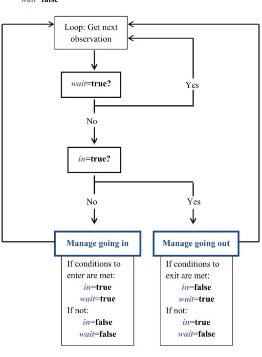
The main idea of the strategy is to take advantage from variations in the stock prices. In this thesis, variations of the stock price are viewed like "errors" as deviations are expected to return to the mean. The strategy is executed for intraday data because there are relevant variations in those intervals and also to increase the number of occurrences of the desired behavior. The way the strategy unfolds is by going observation by observation in a loop. The strategy stops at each 5 minutes interval to do some analysis. It uses a training window, with previous prices, in order to calculate some indicators, which then will be compared with the price of the current observation. Depending on the length of the training window, some observations are lost, since the strategy starts after the first training window. Then, if the strategy decides to go in (buy or sell), it waits one observation, because the order is executed one observation after the decision was made, and then it moves on to the next observation and goes on to checking whether to close the position or to maintain it. If the strategy decides not to go in, it moves on to the next observation but it keeps checking the conditions to enter until it eventually goes in. The procedure that the strategy follows in order to invest is shown in the following diagram.
If conditions to enter are met:
in=true wait=true If not: in=false wait=false If conditions to exit are met:
in=false wait=true If not: in=true wait=false Initialisation: in=false wait=false
in - Boolean type of variable; True if the strategy has a position in the stock (long or short), false otherwise.
wait - Boolean type of variable; It is only true in the moments where the strategy decides to open or close a position; it is there for the purpose of skipping one observation, because once some decision to enter or exit is made, the execution of the trade is made one observation after.
Figure 1 - Diagram showing how the strategy procedure operates.
Loop: Get next observation
in=true?
Manage going in
wait=true?
Manage going out
No
Yes
The average of prices in the training window is used as the reference to what the price of the stock should be. Apart from the mean, the volatility of prices is also obtained from the training window, by calculating the standard deviation. Since the standard deviation is, by definition, the average distance of the observations to their mean, this seems like a good indicator of the profits that the strategy can expect to make. The "entrance distance" will be called to the minimum distance between the current price and the mean that the strategy needs to find in order to buy or sell. If the current price is above the mean, it will sell. If the current price is below the mean, it will buy. The "entrance distance" is defined in relation to the standard deviation, for example it can be 70% or 100% of the standard deviation. Figure 2 shows how the "entrance distance" feature plays out. The black dashed line (horizontal line) represents the mean value that would be calculated from the prices of the training window. The green dashed line (vertical line) is the distance of the current price to the mean. In this case we would be evaluating the observation at the peak (the lines are exemplifications, the values were not calculated). In this case, if the distance to the mean was larger than one standard deviation of the prices of the training window, there would be a sell signal.
Figure 2 - Alphabet stock (GOOGL) during some period on the 19th January 2018.
Another indicator that is used is called in this document a "turning point". Turning point will be when a trend inverts direction. When the strategy buys or sells, I want to know that the stock is going the way I expect it to as soon as possible, so I only open the position when it starts going in that direction. For example, in Figure 2 it would not sell at the peak, it would sell slightly after, when it was already going down. There will be a turning point if:
I considered this indicator useful for this strategy in particular because the strategy uses intraday data, so the trends have a lot of detail, therefore it is possible to see well where they invert. To sum up, the two conditions to enter is having the minimum entrance distance to the mean and having a turning point.
Once the strategy is in, it needs to check the conditions for exiting. Here, it goes observation by observation and it checks the current price against the reference price of when it bought or sold the stock. The expression "profit target" will be used to call the minimum positive distance between the current price and the reference price that one needs to have in order to close the position. The value is calculated differently, depending if the strategy sells or buys. The positive distance is the one that gives a profit. At exit, there is also the "turning point" indicator. It aims to find the places where the trend that was being taken advantage of is finished. The goal of including this is to make sure that we get all the potential from a rise or a fall, to let the stock go as far down or as far up as it will go. Therefore, the strategy will exit if the price is doing the opposite of what the trend was doing. Thus, at exit, there is a turning point if:
If there is a profit equal or higher than the profit target at the same time as there is a turning point, then the strategy will exit. The strategy will also exit if a limit of time is reached from the moment the strategy opened the position until the current observation. The expression used in this document to designate that time limit will be the "maximum duration". Lastly, the strategy can also exit if a certain loss boundary is reached. The maximum loss that the strategy can make will be called the "loss limit".
current price (price at current observation) < previous price (the price is going down)
if current price > training window average (in this case the strategy is about to sell) current price (price at current observation) > previous price
(the price is going up)
if current price < training window average (in this case the strategy is about to buy)
current price (price at current observation) < previous price (the price is going down)
if it bought the stock current price (price at current observation) > previous price
(the price is going up)
There are some risks associated with this strategy. If in fact there are some profits coming from its implementation, and this being because the market does indeed exhibit the behavior that I am looking for, even then there is no assurance that the stock market will continue to exhibit that trend. The stock market is changing over time and a strategy that worked in the past does not necessarily work in the present. Another risk associated with the strategy is noise traders. The actual proposition in which the strategy stands that there are deviations that do not reflect the fundamental price can be turned against the strategy itself, because then, when I consider the fundamental price as being the average of previous prices, I cannot be sure that those previous prices are not themselves deviations from the fundamental price. Because with noise traders, we do not know if the price is at the fundamental value. However, in some way, that is why the average is taken: it gives a more correct estimate of the fundamental price.
Regarding transaction costs, a fixed cost per transaction would not be an impediment for this strategy because the number of shares dealt in a transaction would be increased in order to dilute the transaction costs. Therefore the transaction costs would reduce the profits but would not eliminate them.
Having a turning point feature in this strategy could have been a problem in the past because of the uptick rule, in which one could only sell after there have been two upward movements in the stock, however in 2010 this rule was updated and the restriction is now only applied to the companies that are making a 10% loss in a day. Nevertheless, if the stock dropped 10%, this strategy would buy the stock, instead of selling, so it seems to not make any difference. However, I did not consider this restriction in the tests.
Results
Mean Strategy in the S&P 500
The mean strategy was back-tested for the S&P 500 index. The data used was intraday data with 5 minutes intervals, from the 16th June 2017 until the 23rd January 2018, which is a
dataset with 12,068 observations, however the results shown later are from the 23rd June 2017
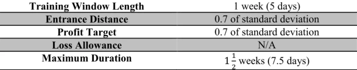
onwards because 390 observations are lost to form the training window. Table 1 provides a summary of the settings used for the test performed on the S&P 500. The number of
observations in the training window was obtained by multiplying 5 days by 78 observations per day. The 'maximum duration' indicator was set at one and a half week, so 585 observations (7.5 * 78 observations). The entrance distance and the profit target were set at 0.7 of the volatility, in an attempt to take advantage of a higher number of variations. These indicators have to do with the size of variations that we are trying to catch and their frequency. A smaller value will include more variations but with smaller amplitude and a bigger value will include the opposite: less variations but with larger distances to the mean.
Training Window Length 1 week (5 days)
Entrance Distance 0.7 of standard deviation
Profit Target 0.7 of standard deviation
Loss Limit N/A
Maximum Duration 11
2 weeks (7.5 days) Table 1 - Settings for the mean strategy executed on the S&P 500 data.
In this test the maximum loss indicator was not used. The way the strategy ended when it did not make a profit was solely through the 'maximum duration' limit. This means the strategy will exit if it exceeds a time limit.
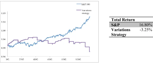
The overall result of the strategy was a negative return of 3.25%. The benchmark (the S&P 500) achieved great results in this period, having made a very high return of about 17% in seven months. The fact that the S&P 500 performed very well in this period was the reason that the variations strategy did not. The S&P showed a very steady rise in about the last four months of this period, and it exhibited few downward variations, therefore the prices did not come back to the mean, which is what we expect it to happen in this strategy. Figure 3 shows the cumulative returns of the variations strategy against the benchmark through time. They were obtained by starting with an initial wealth of 1 and applying the returns successively. The strategy was performing well, and even better than the S&P 500, until around the 25th
September 2017. From then on, it lost value with the consistent rise of the S&P 500 and it terminates with a 3% loss.
Figure 3 - Cumulative returns of both the S&P 500 and the variations strategy and total returns.
Table 2 shows the balance between the Buy and Sell parts of the strategy. From those results we can see that the number of Buy strategies is similar to the number of Sell strategies, which means that the strategy is not preferring any of the two types over the other. For both parts the number of positive returns are higher than negative returns, and for Buy there is only one negative return in 31 returns. This implies that the strategy is right most of the time about where to sell and buy, specifically it is right 97% of the times for buy and 66% for sell. However, the variations strategy exhibits an overall negative return, hence the magnitude of the returns has to be unbalanced. This can be observed in Figure 4, where the separate returns of buy and sell parts are shown. It is possible to note that the big negative returns are coming from the sell part and that this part is responsible for the overall negative performance of the strategy. Moreover, the range for the Sell returns, from -3% to 0.75% is much broader than the one from Buy, from -0.3% to 0.55%, and the negative side is much ampler than the positive side. There is an asymmetry creating a lot of downside risk. This happened because the strategy did not cap the losses but it capped the gains. It was set to stop when a certain profit was reached (a value of 70% of the standard deviation) but when it went badly it only stopped after a maximum duration had expired without having any loss limit.
Table 2 - Results of buy and sell parts in the variations strategy. 'Buy +' is the amount of buy orders with positive returns; 'Buy -' is the amount of buy orders with negative returns; 'Sell +'
is the amount of sell orders with positive returns; 'Sell -' is the amount of sell orders with negative returns. Total Return S&P 16.80% Variations Strategy -3.25%
Buy + Buy - Sell + Sell -
30 1 19 10
Figure 4 - Returns from Buy and Sell parts of the strategy separately.
Taking this unbalance into account, a mean strategy was tested with a maximum loss limit equal to one standard deviation, keeping the other indicators constant. The overall return with this modification was 0.80%. Figure 5 presents the cumulative returns for the strategy in comparison with the S&P 500 and further characteristics of the strategy and the benchmark. The returns of the S&P were statistically significant during this period, whereas the variations strategy's were not and the Sharpe Ratio of the S&P was 0.029, bigger than the strategy's of 0.0178. The reason why the loss limit feature does not give an even better result is because introducing it has the disadvantage that it cuts some of the investments that would otherwise be gains if the strategy waited longer. Here, the loss limit was applied only to the sell side, instead of for both buy and sell. Introducing this limit also changes the pattern of returns quite significantly, with this data. As it is shown in figure 6 and table 3, the number of sell returns is now 109 in total, against the 29 that it was previously. With the steady rise of the S&P 500 from September 2017 in our dataset, the strategy repeatedly thinks that it should sell because the price is above the previous average but then makes a loss.
Figure 5 - Cumulative returns of the variations strategy against the S&P 500 returns (a loss limit of one standard deviation was applied to the strategy) and further characteristics.
Figure 6 - Returns from Buy and Sell parts of the strategy separately (with a maximum loss on the sell side equal to one standard deviation).
Table 3 - Results of buy and sell parts in the variations strategy
A sensitivity analysis was made to verify how the change in parameters would impact the return of the strategy. It tests the different indicators separately considering that everything
Variations Strategy Mean 6.18E-05 Volatility 0.00347 t-stat 0.212 S&P Mean 1.33E-05 Volatility 4.57E-04 t-stat 3.135 Sharpe Ratio S&P 0.029 Strategy 0.0178
Buy + Buy - Sell + Sell -
32 1 46 63
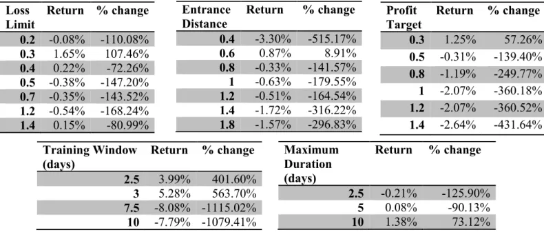
else stays constant. The results are shown in table 4. There are big variations in the returns when we change the parameters. In one way, this shows that the strategy is not very robust in relation to the parameters, but on the other hand some variation was expected because each indicator in the strategy has a meaning and a balance in relation to the others, so by changing each of them we essentially tell the strategy to do something different. One example that changing the parameters can alter the balance of the strategy is the case of the 'entrance distance' indicator. If we reduce the 'entrance distance', it will mean that the strategy buys or sells when small variations are found, but then we kept the profit target constant, so the entrance distance would not have been high enough to generate such big profits. According to this analysis a larger maximum duration of 10 days would increase the return by 73%, to 1.38%, perhaps because it would let the strategy wait for the stock price to go where the strategy wanted and this means that we might be cutting some potential profits in this strategy by exiting early. For a 'loss limit' of 30% of the standard deviation, a return of 1.65% would be obtained. By having a small 'loss limit' while keeping the target profit constant, we are telling the strategy to have smaller losses in relation to the size of the profits. For a training window of 3 days, the strategy achieved a really high return of 5.28%, which tells us that a shorter window is more efficient in this case. A longer time period would have been necessary to see how the strategy reacted to all the different behaviors of the S&P.
Table 4 - Sensitivity Analysis Results. The '% change' column gives the change in percentage from the return that was obtained with the original settings (0.8%). The 'Loss limit', 'Profit
Target' and 'Entrance Distance' are defined in relation to one standard deviation, i.e. the value used in the strategy is the value in the table multiplied by the standard deviation. Loss Limit Return % change 0.2 -0.08% -110.08% 0.3 1.65% 107.46% 0.4 0.22% -72.26% 0.5 -0.38% -147.20% 0.7 -0.35% -143.52% 1.2 -0.54% -168.24% 1.4 0.15% -80.99% Profit Target Return % change 0.3 1.25% 57.26% 0.5 -0.31% -139.40% 0.8 -1.19% -249.77% 1 -2.07% -360.18% 1.2 -2.07% -360.52% 1.4 -2.64% -431.64% Entrance Distance Return % change 0.4 -3.30% -515.17% 0.6 0.87% 8.91% 0.8 -0.33% -141.57% 1 -0.63% -179.55% 1.2 -0.51% -164.54% 1.4 -1.72% -316.22% 1.8 -1.57% -296.83% Training Window (days) Return % change 2.5 3.99% 401.60% 3 5.28% 563.70% 7.5 -8.08% -1115.02% 10 -7.79% -1079.41% Maximum Duration (days) Return % change 2.5 -0.21% -125.90% 5 0.08% -90.13% 10 1.38% 73.12%
The sensitivity analysis revealed that the strategy operates more efficiently for a training window of 3 days, therefore the characteristics with these settings are shown below. The strategy makes a return of 5.28% with a Sharpe Ratio of 0.092.
Figure 7 - Cumulative returns of the variations strategy against the S&P 500 returns (with a loss limit of one standard deviation and a training window of 3 days) and further
characteristics.
This dataset contained one of the situations where the strategy struggles. A risk of the strategy (or something to be aware of) is that the success of it has to do with the pattern that the stocks exhibit, if it is like the one that it looks for. As long as the pattern contains variations, the risk is low. However, if the stocks deviate from the mean for too long (and long here can be weeks or months), there is a risk that the strategy will perform badly. By testing past data we get results as how the data behaved then. Whether or not the stock will exhibit that behavior in the future we do not know.
Buy-Only Strategy in the S&P 500
A Buy-Only strategy is done by only allowing the variations strategy to buy, while keeping all the other rules. I would suggest having a buy-only strategy for the S&P because of the fact that the S&P goes up in trend. There will be the risk from taking a side and the strategy will be exposed to crises or crashes, however the risk of exposure to these events will be the same as that of buying the S&P itself.
The data used for this test was the same as before: the data for the S&P 500 with 5 minutes intervals, from the 16th June 2017 until the 23rd January 2018. The same indicators were used
as for the previous strategy. The maximum loss limit was not applied.
Variations Strategy
Mean 2.82E-04
Volatility 0.00308
Training Window Length 1 week (5 days)
Entrance Distance 0.7 of standard deviation
Profit Target 0.7 of standard deviation
Loss Allowance N/A
Maximum Duration 11
2 weeks (7.5 days) Table 5 - Settings for the buy-only strategy executed on the S&P 500 data.
This strategy gives a return of 8.36%. Although the S&P achieves a larger total return in the period, the characteristics of the strategy overcome those of the S&P: the kurtosis, skewness, and volatility are more attractive for the strategy, since they provide less risk. Hence, the variations strategy has a better Sharpe ratio (1.42) comparing with the S&P (0.029). With 97% of positive returns, the variations strategy shows basically no risk. The volatility here is actually not that relevant because it is volatility between all positive returns. The purpose of having this strategy where we could just buy the S&P 500 is that there is a bigger potential in the difference in prices from the variations of the S&P, rather than just focusing on the total return at the end.
Figure 8 - (1) Graph with Cumulative Returns; (2) further characteristics of the strategy and the benchmark and (3) chart with the magnitude of the returns.
Total Return S&P 16.80% Variations Strategy 8.36% Variations Strategy Mean 0.0024 Volatility 0.0017 t-stat 8.13 S&P Mean 1.3E-05 Volatility 4.6E-04 t-stat 3.14 Buy + Buy - 32 1 33 (2) (3) (1)
If we wanted to protect from the crashes in the S&P, a loss limit could be implemented, and then whenever the S&P dropped more than the limit, the strategy would exit.
A sensitivity analysis was conducted to this strategy. The results are more robust to changes in parameters than the previous strategy and all the returns are positive for whatever values of the indicators. However two indicators impact returns quite a bit. One is the training window. For longer training windows the returns can drop as much as 61%, to 3.26%, as can be seen in table 6. Additionally, the most efficient length for the training window is again 3 days, where the return reaches 9%. The second indicator is the 'entrance distance'. Once again, changing the 'entrance distance' without changing 'profit target' originates big variations.
Table 6 - Sensitivity Analysis Results
Mean Strategy for separate companies in the S&P500
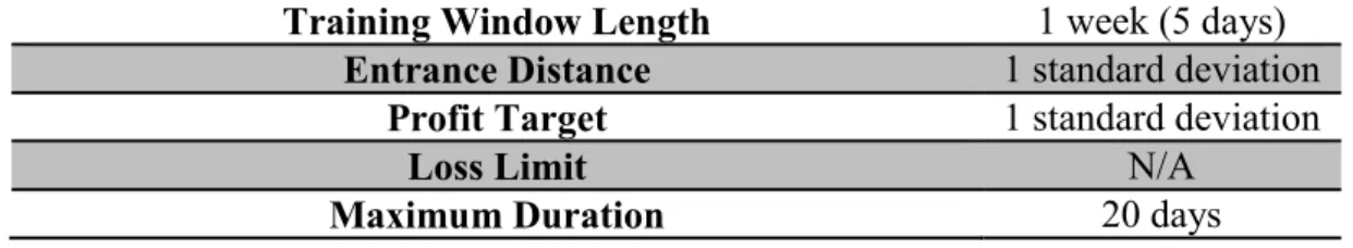
The mean strategy already defined in this document was applied to single companies in the S&P 500. The sample was created by selecting the 30 companies with highest volume in the previous 52 weeks (data obtained on 25th April 2018). Table 7 contains the settings used for
the strategy. There is no loss limit applied and the maximum duration is 20 days. This means that we are giving a lot of freedom to the strategy to wait for the stock price to do what it looks for. Training Window (days) Return % change 2.5 7.63% -8.83% 3 9.04% 8.14% 7.5 3.46% -58.65% 10 3.26% -61.04% Entrance
Distance Return % change 0.4 5.14% -38.54% 0.6 7.03% -15.90% 0.8 7.43% -11.11% 1 5.31% -36.48% 1.2 5.14% -38.50% 1.4 4.67% -44.19% 1.8 3.75% -55.21% Profit Target Return % change 0.3 7.14% -14.65% 0.5 7.30% -12.75% 1 6.51% -22.14% 1.2 7.11% -15.00% 1.4 7.86% -6.07% Maximum Duration (days) Return % change 2.5 6.93% -17.09% 5 7.86% -6.00% 10 8.53% 1.97%
Training Window Length 1 week (5 days)
Entrance Distance 1 standard deviation
Profit Target 1 standard deviation
Loss Limit N/A
Maximum Duration 20 days
Table 7 - Settings for the mean strategy executed on separate companies' stocks.
The results show an overall positive return of 5.60% for the three months of the dataset, from the end of January to April 2018. This result was obtained by taking into account all the returns from all companies in equal weights, as if a person had invested 1/30 of the portfolio in each company. The value is statistically significant. The results show that the strategy creates in fact some value, and it chooses the direction of the investments correctly more often than it gets it wrong. The results are presented in Table 8. The Sell and Buy returns columns were obtained by creating separate cumulative returns for the returns of each type. The sum of the two does not equal the total return of the strategy.
The sell part of the strategy performs better than the buy part. One of the factors that could possibly explain this difference in performance is the return that the company itself has made in the period. The value of the correlation between the returns of the companies and the sell returns was -0.57, and the correlation between the company returns and the buy returns was 0.67. These high values of correlation mean that if the company has a negative return, the sell returns will tend to be higher and the buy returns will tend to be lower. If the company has a positive return, the sell part will tend to perform worse and the buy part will tend to have stronger results. Differently from the case of the S&P 500, here, keeping both parts of the strategy is beneficial given this correlation, because it acts as an insurance where at least one part performs better than the other no better the direction of the stock. Furthermore, in this dataset most companies had negative returns, hence why the sell part performed better.
Table 8 - Results of the mean strategy for a group of 30 companies in the S&P 500. For each company it is presented the return of the variations
Ticker Company Company's Return Variations Strategy % >=0 Returns Buy Returns % >=0 Returns Sell Returns % >=0 Returns AMZN Amazon.com Inc 11.22% 15.17% 92.86% 14.40% 100.00% 0.67% 85.71% AAPL Apple Inc -5.55% -2.97% 71.43% -1.86% 50.00% -1.14% 80.00% FB Facebook Inc -8.43% 3.69% 80.00% -5.25% 60.00% 9.44% 100.00% NVDA NVIDIA Corp -6.92% 32.62% 92.31% 6.74% 83.33% 24.25% 100.00% GOOGL Alphabet Inc -13.38% -3.72% 66.67% -6.70% 50.00% 3.19% 100.00% MSFT Microsoft Corp 1.97% 20.67% 100.00% 9.31% 100.00% 10.40% 100.00% TSLA Tesla Inc -14.06% 17.02% 90.91% 1.03% 83.33% 15.83% 100.00% NFLX Netflix Inc 13.24% -1.90% 92.86% 19.92% 100.00% -18.20% 80.00% BAC Bank of America Corp -6.64% 12.09% 94.74% 3.40% 90.91% 8.40% 100.00% JPM JPMorgan Chase & Co -6.02% 20.00% 100.00% 10.48% 100.00% 8.61% 100.00% C Citigroup Inc -13.92% -5.67% 66.67% -7.64% 50.00% 2.13% 100.00% MU Micron Technology Inc 9.22% -24.62% 80.00% 0.79% 83.33% -25.21% 75.00% INTC Intel Corp 5.14% 16.28% 88.89% 14.19% 100.00% 1.83% 66.67% XOM Exxon Mobil Corp -12.54% 0.20% 80.00% -4.20% 66.67% 4.60% 100.00% BKNG Booking Holdings Inc 9.70% -15.15% 71.43% -0.61% 75.00% -14.62% 66.67% WFC Wells Fargo & Co -20.76% -10.73% 75.00% -13.33% 66.67% 3.01% 100.00% GE General Electric Co -10.90% -7.18% 75.00% -11.60% 60.00% 4.99% 100.00% JNJ Johnson & Johnson -11.69% 2.21% 85.71% -1.36% 75.00% 3.62% 100.00% T AT&T Inc -12.30% 1.19% 75.00% -4.26% 50.00% 5.69% 100.00% AVGO Broadcom Inc -7.19% 30.85% 100.00% 17.03% 100.00% 11.81% 100.00% BA Boeing Co -0.29% 29.31% 94.44% 11.16% 88.89% 16.33% 100.00% CSCO Cisco Systems Inc 4.60% -9.03% 60.00% -4.01% 50.00% -5.24% 66.67%
V Visa Inc -0.39% 11.53% 100.00% 6.02% 100.00% 5.20% 100.00%
DIS Walt Disney Co -11.63% 2.56% 84.62% -2.95% 75.00% 5.68% 100.00% AABA Altaba Inc -13.11% 4.20% 85.71% -1.41% 66.67% 5.69% 100.00% CMCSA Comcast Corp -23.98% -2.86% 87.50% -11.61% 71.43% 9.90% 100.00% AMGN Amgen Inc -10.88% 19.73% 94.74% 8.56% 88.89% 10.29% 100.00% CELG Celgene Corp -12.88% 14.64% 84.62% 1.28% 71.43% 13.19% 100.00% HD Home Depot Inc -9.58% 1.82% 83.33% -3.84% 71.43% 5.89% 100.00% WMT Walmart Inc -19.54% -4.04% 84.62% -9.84% 75.00% 6.44% 100.00%
In order to see how the strategy fitted in the data, the graphs with the stock price, as well as buy, sell, and exit signals were analyzed for the companies where the mean strategy performed best and worst. These companies were respectively NVIDIA Corp and Micron Technology Inc. The graphs are presented in Appendix B, along with charts showing the separate "buy" and "sell" returns for these companies. Micron presented several situations where the price kept going up repeatedly. This poses a challenge for this strategy. If the companies are in a period where they are growing immensely, the strategy will wait one month for the price to come back to the mean and will make a big loss. This is the disadvantage of waiting for the stock to go in the right direction: when it is wrong, it is costly. Perhaps to improve performance one could couple the strategy with research and actually choose stocks that he knows are not exposed to such growth. Or one could look at the recommendations for different stocks and only select the ones that have neutral recommendations and leave out the ones that have strong sell and buy recommendations. Steady rises (and steady drops) are a big risk for this strategy because the price will go up (down) but will not come back down (up), or at least will not do it as fast as the strategy requires it to. For Micron on 9th March the strategy had a loss of 28.7% because Micron's
stock price kept going up in the month previously to this date. For the whole portfolio this made up a loss of 1.03%. The strategy should find a way to stop early when there is a steady movement, to cut losses. Nevertheless, the way it is defined here still seems to be, in practice, the best way to take advantage of the variations in the stock using the parameters that I described. If I introduced a loss limit of one standard deviation, the strategy would only make 1.47% for the same period, with a lower Sharpe ratio and the returns would not be statistically significant. The loss limit would not work too well for separate companies as it works for the S&P, because since there is a lot of volatility in stocks, any sudden variation can trigger the strategy to exit, which is not optimal. If I applied an absolute loss limit of 10%, for example, with which the strategy could not make a loss bigger than that value at any point, the strategy would make 3.31% with no less volatility.
In both Micron and NVIDIA strategy performances there is one further point that is not perfect. When the strategy takes a side and it is temporarily wrong, it waits for the stock price to go its way and in the meantime there are variations and potential profits that are being missed. Actually, in the dataset there seem to be a lot of opportunities of the behavior that the strategy looks for, so it is difficult to catch all of them, especially having fixed profit targets. Even so, the strategy is doing a good job. Another important point to note is that in this
dataset there are companies that had their earnings reports, which introduces the factor of information that changes stock prices and affects the performance of the strategy. Micron's earnings report was on the 22nd March 2018, so the rise could have been due to expectations
of a good result.
If a person had invested in all companies in the sample with equal weights, the return he would get would be the one stated before: 5.6%, and the Sharpe Ratio would be 0.023. The cumulative returns and further characteristics are shown in figure 9. The strategy makes a lot of small gains and shows a consistent rise overall, although there was a crash around 9th
March 2018 (observation 5353), which was in fact due to two consecutive drops: a 1.03% loss from Micron and a 0.9% loss from Netflix. The problem for Netflix was the same as for Micron: the stock price rose immensely and the strategy waited one month and then exited with a very large loss (25% drop for the value of the sub-portfolio, 0.9% for the whole portfolio). In Appendix B there are also the graphs with the stock price of Netflix, buy, sell and exit signals for the period of the loss. The performance of the strategy is attractive even with the crash because the gains overcome the losses and the value of the portfolio in the three months was always bigger or equal to the initial wealth. Moreover, an investor could even add more companies to the portfolio, to reduce the impact that a single one has on the wealth. There would be less risk for the whole portfolio if one company rose a lot in one day in that case, since it could only impact up to a certain value in the whole portfolio. With 30 companies this limit was at 3.3%. Comparing to the benchmark, the variations strategy had a really good performance, making 5.6% in the same period as the S&P 500 had a negative return of 6.44% and the companies in the sample made a negative return of 6.58% on average.
Figure 9 - Performance of the variations strategy.
Variations Strategy Mean 4.80E-06 Standard deviation 2.12E-04 t-stat 2.42 Sharpe Ratio 0.0227
If the investor had preferred to choose one stock separately, then he could have gotten any of the different returns in Table 8. The distribution of those returns are shown in Figure 10. The normal distribution is centered at 5.6%. There are overall more positive returns than negative returns and the highest returns are bigger in magnitude than the lowest returns. The distribution only shows how the returns would look like in a point in time in relation to each other. However, I believe these results would be different for a longer time period, because the companies can recover from a bad performance. It is not the case that one single company will perform poorly forever nor the opposite. The performance varies for each company.
Figure 10 - Distribution of returns of the 30 companies in the sample.
A sensitivity analysis was made to the strategy, by changing each parameter separately while keeping all the others constant. This strategy is, to some degree, robust to the change in parameters, especially when comparing with the mean strategy for the S&P studied previously in this thesis. The returns change a lot, by between -35% and 49% however, this is because when changing the parameters the dynamics of the strategy changes, and the variations that the strategy catches are different. All the returns are positive and vary between 3.63% and 8.35%; most of them are statistically significant for 5% and some of them are so even for 1% significance.
Table 9 - Sensitivity Analysis Results
I also analyze the returns by sectors. The biggest movements are associated with Technology companies such as Micron, NVIDIA, Microsoft, Intel and Broadcom, perhaps because Technology companies grow fast and they innovate constantly, being able to originate large increases in revenues. The other explanation (and perhaps for the same reason) is that there can be a big interest by investors in trading these stocks. The Services sector in this period performed worst, loosing 0.88% and the best sector was Healthcare with an average return of 12.19%. There are no companies from the Utilities nor the Conglomerates sector in the sample and there is only one company in the Basic Materials, so there cannot be significant conclusions about the performance of the strategy for those sectors.
Figure 11 - Distribution of returns by sectors. Entrance Distance mean std dev t-stat % change 0.4 4.41% 0.134 1.807 -21.3% 0.6 5.57% 0.132 2.313 -0.5% 0.8 5.89% 0.147 2.195 5.2% 1.2 6.80% 0.139 2.686 21.4% 1.4 4.67% 0.117 2.191 -16.6% Profit Target mean std dev t-stat % change 0.4 5.17% 0.131 2.152 -7.7% 0.6 6.17% 0.138 2.443 10.2% 0.8 6.55% 0.151 2.377 17.1% 1.2 5.44% 0.136 2.196 -2.9% 1.4 4.72% 0.133 1.942 -15.7% Maximum Duration (days)
mean std dev t-stat % change 10 3.63% 0.109 1.820 -35.2% 15 5.55% 0.162 1.872 -0.9% 25 4.52% 0.154 1.606 -19.2% 30 4.65% 0.160 1.595 -16.9% 40 8.32% 0.128 3.558 48.7% Training Window (days) mean std
dev t-stat % change 2 8.35% 0.156 2.928 49.1% 3 6.07% 0.126 2.649 8.5% 7 7.12% 0.124 3.148 27.1% 10 5.64% 0.113 2.732 0.7% Sectors Average Return Basic Materials 0.20% Conglomerates - Consumer Goods 7.03% Financial 5.24% Healthcare 12.19% Industrial Goods 11.07% Services -0.88% Technology 5.28% Utilities -
The correlation between the volatility and the return of the variations strategy for the stocks was 0.037, therefore there is not a big effect of volatility on the returns overall, possibly because it affects both positive and negative returns, which then cancel out.
The risks of this strategy have to do with whether the stock market will keep behaving in the way it did in the past, and particularly for this strategy, the stocks need to exhibit more variations than they exhibit periods of steady growth for it to yield positive returns. As for the crashes, this thesis did not study the behavior of the strategy in the presence of those events. The behavior will depend on whether the strategy is at a sell or buy moment when the crash happens. However, once the value of the stocks stops dropping and starts rising slightly, then, there will be a 'turning point' and the strategy will exit. However, during the crash, the prices will lead to buy signals, as the current price will be smaller than the mean, and this could originate big losses, as when the prices grow steadily.
Conclusion
I defined a strategy that takes advantage of short variations in stock prices, by assuming that deviations will return to their mean. Firstly, the strategy was applied to the S&P 500. The results were not very robust and it is difficult to defend that they have significant positive returns. Even for a training window of 3 days, where the strategy would have had a big return of 5.28%, this result was already obtained by changing the original strategy. And there were other changes in the strategy that would have originated negative returns, hence why we cannot be sure of its viability. The strategy performed badly in this period because the S&P made a constant rise of 17%, which is not so common, so the strategy could still recover afterwards if we looked at a longer time window. Furthermore, the strategy was outperforming the S&P before it started going up, which shows that it does a good job creating value when there are variations, and that this value grows fast. However, the way the strategy is made is at the cost of loosing when there is a steady movement in the index. By investing in person instead of by running the algorithm, these risks could be mitigated, because the investor would recognize when the stock was going up and would stop looking for variations then. However, to implement this strategy, a person would need to monitor the movements closely, which is a big spending in resources. I suggested a Buy-Only strategy for the S&P, given the trend that the S&P rises in the long run. The strategy would try to profit from variations but only upward ones. This gave a Sharpe ratio of 1.42 for the period from
June 2017 to January 2018 (7 months). We are taking a directional position here and the strategy is then exposed to crashes, however it is no greater risk than that of buying the S&P 500 itself.
The usual motivation for investing in an index is to reduce risk, by smoothing the small cycles that each separate company exhibits. Nevertheless, these 'small cycles' in the companies' stocks, the variations around the same value is what the mean strategy looks for, hence, it should preferably be executed in separate stocks. The results agree with this. The strategy gave a return of 5.6% (statistically significant) from the end of January 2018 to April 2018 (3 months) with a Sharpe ratio of 0.0227. However, this is by creating a portfolio with the 30 stocks tested. If we had looked at their separate performances, some of the stocks would exhibit large losses. These stocks present the behaviors which the strategy does not predict. The portfolio with all stocks works better because it sums all the returns and in this period the amount of profits was bigger than the losses for the whole sample. For separate stocks both the sell and buy parts of the strategy are beneficial and would complement each other, since the buy part has a large positive correlation with the stock returns and the sell part has a large negative correlation. The main issue that the strategy finds is when the stocks exhibit steady rises; when they are growing a lot and they overcome maximums in short periods of time, without coming back down. In the 3 months of the dataset, the return of the strategy was positive because the undesired behavior did not happen too often, nor for many companies. So positive results in the future will depend on the stocks exhibiting a similar behavior than it did in this period.
A possible improvement of the strategy would be to become more dynamic. For example, when the company stock is rising consistently, it could identify so, and exit early. For that, I would perhaps need to use some techniques to recognize patterns visually, or mathematical techniques to define the behaviors. The strategy could also be improved to increase the control over some situations, take more information into account and react differently in distinct moments. One particular part of the strategy that could be improved is at exit. We could include either a volume indicator or a slope indicator to know whether there is a pressure for the price to go up or down, and therefore decide to wait a little longer or to close the position accordingly, instead of exiting at a fixed target. The slope could also be used as an indicator of whether the price is going up or down, because a big slope is indicative of an action that a lot of people are doing, and sometimes those trends are self-fulfilling, like in crashes. I also talked about introducing information. In improving the performance of the
strategy by selecting purposely the stocks that an investor knows are not about to grow or to decline immensely, but rather are likely to stay around a value; and exclude companies whose earnings report is approaching. Additionally, we could add more and more companies to the portfolio. This would reduce the risk, given that the companies exhibit in general less steady growths (undesired behavior) than variations around the mean (desired behavior).
The strategy works well because it takes advantage of an occurrence that can happen, by specifying the strategy in order to look for it and wait for it. The results in this period show statistically significant returns, meaning that in the past, the behavior that we aim at has existed in the stocks. If an investor would use the guidelines in this thesis would be because he would believe that because of their nature, stocks will always exhibit considerable volatility and therefore will always exhibit variations around the mean. However, the amount of times that the undesired behavior (steady rises) occurs cannot be dominant over the amount of occurrences of the behavior that we look for. If the stock behaves like in the period that we tested, then the overall gains will be enough to cover the losses and the strategy will be profitable. It would be interesting to follow the strategy for a longer time period, to make significant conclusions on whether this effect would persist with time or cancel out.
Appendices
APPENDIX A
Ticker Company Sector Number of
Observations
AMZN Amazon.com Inc Services 11779
AAPL Apple Inc Consumer Goods 11658
FB Facebook Inc Technology 11540
NVDA NVIDIA Corp Technology 11333
GOOGL Alphabet Inc Technology 9845
MSFT Microsoft Corp Technology 10409
TSLA Tesla Inc Consumer Goods 11083
NFLX Netflix Inc Services 11206
BAC Bank of America Corp Financial 9924
JPM JPMorgan Chase & Co Financial 8592
C Citigroup Inc Financial 7993
MU Micron Technology Inc Technology 11336
INTC Intel Corp Technology 9911
XOM Exxon Mobil Corp Basic Materials 8166
BKNG Booking Holdings Inc Technology 6235
WFC Wells Fargo & Co Financial 7319
GE General Electric Co Industrial Goods 10288
JNJ Johnson & Johnson Healthcare 7213
T AT&T Inc Technology 8211
AVGO Broadcom Inc Technology 7249
BA Boeing Co Industrial Goods 9928
CSCO Cisco Systems Inc Technology 8513
V Visa Inc Financial 7980
DIS Walt Disney Co Services 8133
AABA Altaba Inc Financial 6132
CMCSA Comcast Corp Services 6419
AMGN Amgen Inc Healthcare 6303
CELG Celgene Corp Healthcare 7324
HD Home Depot Inc Services 7795