Calendar Effects in Stock Markets: Critique of Previous Methodologies and Recent Evidence in European Countries

Carlos Pestana Barros & Nicolas Peypoch

A Comparative Analysis of Productivity Change in Italian and Portuguese Airports

WP 006/2007/DE _________________________________________________________

Maria Rosa Borges

Calendar Effects in Stock Markets: Critique of Previous

Methodologies and Recent Evidence in European

Countries

WP 37/2009/DE/UECE _________________________________________________________

Department of Economics

W

P

ISSN Nº0874-4548

School of Economics and Management

Calendar Effects in Stock Markets:

Critique of Previous Methodologies

And Recent Evidence in European Countries

Maria Rosa Borges mrborges@iseg.utl.pt

ISEG (School of Economics and Management) of the Technical University of Lisbon

Rua do Quelhas, 6 1200-781 Lisboa

Portugal

UECE (Research Unit on Complexity and Economics) Rua Miguel Lupi, 20

1249-078 Lisboa Portugal

1

Calendar Effects in Stock Markets:

Critique of Previous Methodologies

And Recent Evidence in European Countries

Abstract

This paper examines day of the week and month of the year effects in seventeen European stock

market indexes in the period 1994-2007. We discuss the shortcomings of model specifications and

tests used in previous work, and propose a simpler specification, usable for detecting all types of

calendar effects. Recognizing that returns are non-normally distributed, autocorrelated and that the

residuals of linear regressions are variant over time, we use statically robust estimation methodologies,

including bootstrapping and GARCH modeling. Although returns tend to be lower in the months of

August and September, we do not find strong evidence of across-the-board calendar effects, as the

most favorable evidence is only country-specific. Additionally, using rolling windows regressions, we

find that the stronger country-specific calendar effects are not stable over the whole sample period,

casting additional doubt on the economic significance of calendar effects. We conclude that our results

are not immune to the critique that calendar effects may only be a “chimera” delivered by intensive

data mining.

JEL codes: G10, G14, G15

1. Introduction

Several empirical studies have studied the phenomena of calendar effects in stock markets, where

returns tend to show higher (or lower) than average returns is specific calendar periods. The calendar

effects that have attracted more interested, fueled by favorable evidence, are: (i) the weekend effect,

where Monday returns tend to be lower than on other days of the week, and sometimes Friday returns

are higher; and (ii) the January effect, revealed in the fact that daily returns tend to be higher in this

month, than in other months of the year. Other calendar effects that have been studied include day of

the month effects, where higher returns tend to be concentrated in specific periods of the month, and

holiday effects, where we observe the behavior of returns after holidays (no trading days).

The study of calendar effects is relevant, in financial economics, because some types of calendar

effects are inconsistent with the efficient market hypothesis. If the flow of information is continuous,

and prices reflect all information, we would expect to find that Monday returns are around three times

higher than other weekday returns, because there are three calendar days between the market closing

of Friday, and the market closing of Monday. But even if we admit that the flow of information is

negligible on weekends, Monday returns should at least be as high as other weekday returns. However,

none of these two hypotheses is confirmed in the US market, nor in several other markets. Monday

returns are in fact lower than other weekday returns. On the other hand, month effects are not

necessarily inconsistent with market efficiency, because it is possible that the flow of information to

the markets is specially concentrated in one, or some, of the months of the year. In any case, there is

no strong evidence that January higher returns are caused by a relatively higher flux of good news, and

so calendar effects remain at odds with both the hypothesis of: (i) market efficiency and (ii) rational

behavior of investors. The study of calendar effects is also relevant for financial managers, financial

counselors, market professionals and investors in general, and all those interested in developing

This paper looks exclusively at day of the week effects and month of the year effects, in European

stock markets. It makes several contributions to the literature on calendar effects in stock market

returns. First, we discuss the shortcomings of previously used models for the detection of calendar

effects, and we propose a simpler model specification that overcomes those shortcomings. Second, we

recognize non-normality and autocorrelation in stock market returns, and time-dependent variance of

the residuals of linear regressions, and apply appropriate statistical methodologies to tackle these

problems, including the bootstrap approach and the GARCH model, adding statistical robustness to

our results. Third, we examine the time-stability of the most significant calendar effects in the period

under study. Fourth, we use observations from a set of seventeen countries of the same economic

region, allowing us to conclude if calendar effects are across-the-board effects in that region or only

country-specific effects. This is important to know, because some possible explanations for calendar

effects, like psychological traits of investors, would imply across-the-board effects, while other

explanations, like those related to fiscal motivations or market structure, allow for country-specific

calendar effects. Five, we use data from recent years, from 1994 to 2007, on West and Central

European stock markets, thus adding and updating international evidence on calendar effects.

The remainder of the paper is organized as follows. In section 2, we present some of the more relevant

previous studies and results on day of the week effects and month of the year effects. In section 3, we

present the data, including several descriptive statistics. In section 4, we discuss alternative model

specifications and their shortcomings, and the different statistical methodologies we use for estimating

the calendar effects. Section 5 contains the results of the model estimations and also includes an

examination of the time-stability of the detected calendar effects. In Section 6, we present the

conclusions and suggestions for further research.

2. Literature Review

Many researchers have studied the phenomenon of seasonalities in price movements in stock markets,

commonly studied calendar effects, which we also cover in the present study are: (i) the day of the

week effect, and (ii) the month of the year effect. There are several studies which focus on other types

of calendar effects, like the behavior of daily returns after holidays, or the behavior of returns in the

first trading days of each month, but those are beyond the scope of this paper. In this section, we

present a short review of previous works on day of the week and month of the year effects, and of the

results they find.

2.1. The day of the week effect

Cross (1973) is among the group of authors that first studies a day of the week effect, namely, the

weekend effect. He observes several US market indexes, without performing statistical tests, and finds

that stocks have a negative return over the weekends. French (1980), Keim and Stambaugh (1984),

Rogalski (1984), and Smirlock and Sarks (1986) examine the Standard & Poor’s and the Dow Jones

Index and conclude that Monday returns are on average negative. However, Rogalski (1984), using

OLS regressions, F-tests and t-tests, observes that the Monday effect is negative but not statistically

significant. In the nineties, Chang et al. (1993) and Kamara (1997) confirm the validity of the weekend

effect.

Using the same approach as Rogalski (1984), other authors, including Jaffe and Westerfield (1985a,

1985b), Condoyanni et al. (1987) and Chang, et al. (1993), study non-US markets, including Japan,

Singapore, Australia, Canada, UK, and other European countries, and find that Monday returns are on

average negative and statistically significant. Other studies find a day of the week effect in different

days. Brooks and Persand (2001) observe significant negative returns on Tuesdays in Thailand and

Malaysia, and a significant Wednesday effect in Taiwan. Jaffe and Westerfield (1985a) and Dubois

and Louvet (1996) confirm that daily returns in some Pacific countries tend to be negative on

This apparent consensus is challenged by a set of more recent studies. Sullivan, Timmermann and

White (2001) use a non traditional approach (a bootstrap procedure) and conclude that calendar effects

no longer remain statistically significant. Rubinstein (2001), Mabberly and Waggoner (2000), Schwert

(2001), Steeley (2001), Kohers et al. (2004) and Hui (2005) undertake international studies and show

that this market anomaly is recently becoming weaker, particularly in developed markets. More

recently, Chukwuogor-Ndu (2006) analyze the day of the week effect in stock market returns in fifteen

European countries and finds corroborative evidence in only seven of those markets. He also finds

significant negative returns on Tuesdays, in some of these countries. Basher and Sadorsky (2006),

using different models for detecting the day of the week effect, conclude that a majority of the twenty

one emerging stock markets they examine do not have such an effect, but some countries do exhibit

strong day of the week effects, even after considering for conditional market risk. Overall, there is

mixed evidence on day of the week effects, as more recent studies, using more advanced statistical

procedures, have cast some doubt on the favorable evidence from the initial studies.

2.2. The month of the year effect

A month of the year effect exists if returns tend to be higher or lower in a specific month, when

compared with the other months of the year. The most commonly reported month effect is the

tendency for returns to be higher in January, although other month effects have also been reported.

The first studies, by Rozeff and Kinney (1976), Dyl (1977) and Brown et al. (1983) analyze the US

stock market and observe significant higher returns in January than in the other months of the year.

Also, Gultekin and Gultekin (1983) study seventeen countries using both non-parametric and

parametric tests, and conclude that January returns are significantly higher when compared with the

other months, in thirteen of those countries.

Keim (1983) links the January effect to a small-firm effect, and a set of international studies find that

small firms achieve larger rates of returns than larger firms, and that this is particularly evident in

largely due to the behavior of prices of small firms, and related to a tax-loss selling hypothesis as

proposed by Brown, et al. (1983), who argues that selling pressure at the end of the tax year depresses

price that rebound back in January. A study of the UK market by Menyah (1999) finds an April effect

for small firms, besides a January effect for larger firms.

Ho (1990) examines twelve stock markets, including Australia, Japan, Korea, New Zealand,

Singapore, Thailand, UK and US, and finds evidence corroborative of the January effect as he

observes that average returns on January are higher than other months at a 95% level of confidence.

More recently, Haugen and Jorion (1996), Tonchev and Kim (2004) and Rosenberg (2004) reach

empirical findings similar to prior studies. In balance, the evidence of a January effect is mostly

confirmatory, although the reasons why it exists are still under discussion.

3. Data

We collect from Reuters daily data on seventeen Western and Central European stock market indexes,

for the period beginning in January, 1994 through to December, 2007. The countries and respective

stock market indexes are, in alphabetical order: Austria (ATX), Denmark (OMXC20), Finland

(OMXHPI), France (CAC40), Germany (DAX), Greece (ASE), Hungary (BUX), Iceland (OMXIPI),

Ireland (ISEQ), Italy (MIBTEL), Netherlands (AEX), Norway (OSEAX), Poland (WIG), Portugal

(PSI20), Spain (IBEX), Switzerland (SMI) and United Kingdom (FTSE).

For all indexes, daily returns are computed as:

(

)

= _{t t}

t P P

r (1)

Where rtis the daily return of the stock market index and Pt is the stock index at date t. When the stock

market is closed on a weekday, we do not compute the daily return both for that day and for the

with a lag of one calendar day, except Mondays, which have a lag of three calendar days. This results

in an average of 3430 observations per country, with a maximum of 3595 observations for the United

Kingdom and a minimum of 3279 observations for Poland. The descriptive statistics for daily returns

of all seventeen stock market indexes are presented in Table 1.

INSERT TABLE 1

From Table 1, we find that the mean daily returns range between 0.016% in United Kingdom and

0.089% in Iceland. In that fourteen year period, the maximum daily returns have been registered in

Finland (+14.6%), Hungary (13.6%) and the Netherlands (+ 9.5%), while the minimum daily returns

happened in Hungary (-18.0%), Finland (-17.4%) and Poland (-11.3%). The standard error of the

mean is lower in Iceland (0.0001313), Portugal (0.0001691) and the United Kingdom (0.0001751),

suggestive of lower return volatility, and higher in Finland (0.0003283), Poland (0.0003026) and

Hungary (0.0002907), a signal of relatively higher volatility. The 90th percentile daily return ranges

from 0.87% in Iceland to 2.02% in Finland. The 10th percentile daily return ranges between -2.05% in

Finland and -0.65% in Iceland. Figure 1 confirms, visually, that Finland, Hungary and Poland had

wider ranges between the 10th and the 90th percentile, and the narrower ranges were in Iceland,

Figure 1

10th and 90th Percentiles of Daily Returns by Country (1994-2007)

In all countries, the distribution of returns is negatively skewed, which means that the left tail

(negative returns) concentrates more extreme observations than the right tail. Kurtosis ranges from 5.3

in Denmark to 16.3 in Hungary. In all cases, kurtosis is above 3, which is the expected value for a

normal distribution. Thus, all daily return distributions are leptokurtic, meaning that relative to normal

distributions, they have both higher peaks and fatter tails (a higher probability of extreme values). The

non-normality of the daily returns distributions is also confirmed by Jarque-Bera, Shapiro-Wilk and

Shapiro-Francia tests, at least at a 1% significance level, for all countries.

4. Methodologies

The approach we use in this paper is to analyze daily returns of stock market indexes, comparing the

daily returns on specific calendar periods, such as the day of the week and the month of the year, with

the daily returns of the remaining days, outside the period under scrutiny. Calendar effects can be

studied either using observations of returns of individual stocks of a specific country, or by examining

the behaviour of a stock market index (as in French, 1980, Keim and Stambaugh, 1984, Rogalski,

1984, Chang et al, 1983, Basher and Sodorsky, 2006). Officer (1975) claims that calendar effects are

4.1. Discussion of the model specification

When using stock market indexes, a common approach in the literature consists in estimating the

following formula. We present the case for the study of the day of the week effect, coding Monday as

1, Tuesday as 2, Wednesday as 3, Thursday as 4 and Friday as 5:

t t t

t t

t D D D D

r =

α

β

β

β

β

ε

Where rtis the daily return of the stock market index, Ditare dummy variables which take on the value

of 1 if the corresponding return for day t is a Tuesday, Wednesday, Thursday or Friday, respectively

and 0 otherwise. Because the dummy for Monday is missing, the constant captures the mean return

on Mondays; *iare coefficients which represent the mean excess daily returns on the remaining days

of the week, relative to Mondays; finally, t is the error term.

In this specification, the t-tests of the *i coefficients inform us if they are statistical significant, i.e., if

the excess daily returns on Tuesdays, Wednesdays, Thursdays and Fridays, either positive or negative,

are significantly different from Mondays’ mean return. If we hold an a priori belief that an effect

exists on one of the specific days, say Monday, this is the best specification. However, if we have no

previous expectation on which of the days a calendar effect might exist (or not), the above

specification is no longer appropriate. For example, if we want to investigate whether a Thursday

effect exists, in the above specification, the coefficient *4would inform us if Thursdays’ returns are

statistically different from Mondays’ returns, but the model tells us nothing whether Thursdays are

different from Tuesdays’, Wednesdays’ and Fridays’ returns. This shortcoming can be overcome by

estimating five different models, one for each day of the week, in each case omitting the dummy

But if our purpose is to test a Monday effect, it might be more appropriate to test the mean daily return

of that day against the mean daily return of the pool of all non-Monday days, instead of testing

Mondays separately against each of the other weekdays. We believe it makes more sense to recognize

a Monday effect, if we find out that the mean daily return of that day differs significantly from the

mean daily return of non-Mondays, rather than in the case where we find out that Mondays differ from

Wednesdays and Thursdays, but not from Tuesdays and Fridays. If, for example, only the coefficient

*

4 in equation (4) is found to be significant, did we find a Monday effect, or a Wednesday effect?

An alternative specification is to include the dummy variables for all weekdays (all five of them) while

excluding the intercept, in order to avoid the dummy variable trap,

t t t

t t

t

t D D D D D

r =

β

β

β

β

β

ε

In this case, the icapture the mean daily return for each of the days of the week, but the t-tests for

those coefficients only inform us if they are significantly different from zero. If the time period under

study is sufficiently long, it is to be expected that mean daily return is positive, whilst a very small

number2. Therefore, the significance of the t-tests is biased in favor of accepting positive excess

returns, and against accepting negative excess returns. This specific bias can be corrected if we

construct our data set with excess daily returns, instead of daily returns.

However, there would still remain a bias, if the excess returns are constructed by deducting the mean

daily returns for the all sample. For example, the excess return on Mondays would not be relative to

non-Mondays, but rather relative to all days of the week including Mondays. A simple example

illustrates this. Suppose we have the same number observations for each of the days of the week, and

that the mean returns for Mondays through Fridays are: 0.001, 0.02, 0.02, 0.02 and 0.02, respectively.

2

The overall mean return is 0.0162, while the mean return for Non-Mondays is 0.02 and the mean

return including Mondays but excluding one other day of the week is 0.01525. By deducting the

overall mean return, we have the following excess returns: -0.0152 for Mondays and 0.0038 for all

other weekdays. By deducting the other-day means returns, we obtain the following excess returns,

instead: -0.019 for Mondays and 0.00475 for all other weekdays. By using the overall mean daily

return to calculate excess daily returns, we would underestimate the absolute value of the excess

returns relative to other days, thus biasing the analysis against the detection of existing calendar

effects.

We claim that a simpler approach, which overcomes all these shortcomings, is to estimate five

equations separately, each aiming to detect a specific day of the week effect:

t it i

t D

r =

α

β

ε

With this specification, if we include only the dummy variable for Mondays, captures the mean daily

return of non-Mondays, and 1 is the excess return of Mondays, relative to non-Mondays. The t-test of

1 tells us if this effect is significant. The same arguments apply to 2, 3, 4 and 5, for detecting other

days of the week effects. Note that an OLS regression of this equation is formally identical to

performing a two-group mean comparison test between the mean daily return of a specific weekday

and the mean daily return of all other weekdays.

All the previous discussion can be transposed to month effect analysis, where the only difference is

that we need twelve different dummies, Mi (i=1 to 12), each taking on the value of 1 if the

corresponding return for day t is of January, February, through December, respectively and 0

otherwise. With this approach, month effect analysis is more burdensome, because we need to

This model specification is so general, that any specific calendar effect can be studied this way, like

for example, the trading days after holidays, the trading days between Christmas and New Year, the

first five trading days of each month, the first one hundred days after a new President elected, and so

on. We just need to construct the dummy variable to take the value of 1 in the relevant days.

4.2. Estimation procedures

The first studies of calendar effects (French, 1980, Gibbons and Hess, 1981, Jaffe and Westerfield,

1985) employ the linear regression model (OLS) which assumes that the data are normally distributed,

serial uncorrelated and with constant variance (Wooldridge, 2003). Connolly (1989, 1991) points out

several specific problems that may arise when using this approach: (i) the stock market index returns

are likely to be autocorrelated (ii) the residuals are possibly non-normal; (iii) and the variance of the

residuals may not be constant.

It is a well documented fact that financial market returns suffer time-dependent changes in volatility

(Fama, 1965, Lau et al., 1990, Kim and Kon, 1994). Engle (1982) proposes the use of autoregressive

conditional heteroskedasticity (ARCH) models in order to correct the variability in the variance of the

residuals. These models assume that the variance of the residuals

( )

σ

that the error term can not be modeled

ε

(

σ

)

generalized version of these models (GARCH) is developed by Bollerslev (1986), where the variance

of the residuals is expressed as the sum of a moving-average polynomial of order q on past residuals

(the ARCH term) plus an autoregressive polynomial of order p, on past variances (the GARCH term):

= − = − + + = p i i t i q i i t i t 1 2 1 2 0

2

_α

_α

_ε

_λ

_σ

The simplest form is GARCH (1,1), which is estimated by maximum likelihood, and includes only one

lag both in the ARCH term (last period’s volatility) and in the GARCH term (last period’s variance).

In more recent studies, different versions of the GARCH model have been used by several authors in

the study of calendar effects (Choudry, 2000 and Chen et al., 2001). Choudry (2000) applies the

GARCH model to a research on a day of the week effect in seven East Asian countries. By analyzing

the estimated coefficients of the dummy variables and coefficients, he finds significant effects in three

of those countries, and also in ARCH and GARCH terms.

In this paper, we aim to detect calendar effects in the following cases, with no a priori restriction on

which periods those effect might be revealed: (i) month effects and (ii) day-of-the-week effects. We

first address the problem of heteroskedasticity by regressing the models in Stata 10 software, with the

option of robust standard errors switched on. The non-normality of the data is tackled by applying the

non-parametric bootstrap approach, with 1000 replications for each model regression, and then using

the standard errors and confidence intervals resulting from the distribution of the estimated

coefficients. The use of the bootstrap approach in the study of calendar effects has been applied before

(Sullivan, Timmermann and White, 2001). We perform a test of ARCH effects on our data, and

confirm that it is present in the data for all seventeen countries. Therefore we re-estimate all our

models with the GARCH(1,1) approach.

5. Results

Considering the discussion in the previous section, we use the following procedures to detect calendar

effects in the daily returns of all seventeen stock market indexes, in the period 1994 to 2007. All

5.1. OLS regressions

We start by computing individual OLS regressions for each of the seventeen countries, using model

(4) for day of the week effects and (5) for month effects. Therefore, we perform a total of 85

regressions for day of the week effects and 204 regressions for month effects. Given the non-normality

of the data, all OLS regressions were computed with robust standard errors. The results for the i

coefficients are presented in Table 2.

INSERT TABLE 2

One of the important critiques to previous studies of calendar effects, is that it may well be exclusively

a result of data mining (Sullivan, Timmermann and White, 2001), based on the idea that if we squeeze

a particular sample or time series hard enough, all sorts of regularities may start to appear. To control

for data-snooping, Cooper, McConnell and Octchinnikov (2006) propose a randomized-bootstrap

procedure, and Schwert (2003) suggests the use of data from other countries.

Our first results, in Table 2, are not immune to the critique of Sullivan, Timmermann and White

(2001). In day of the week effects, the number of significant coefficients is 2 at the 1% significance

level, 6 at the 5% and 5 at the 10%. Given that we compute 85 regressions, the number of significant

coefficients that we might expect to find, in random data, would be around 1 (at 1%), around 4 (at 5%)

and around 8 (at 10%). So, our overall results for day of the week effects are not very different from

those we might expect to obtain, in a randomly constructed sample. For month effects, the number of

significant coefficients is 6 (at 1%), 10 (at 5%) and 18 (at 10%). As we have 205 regressions, again,

our global results are similar to the number of significant coefficients we might expect to find in

random data at 5% (10) and 10% (20). However, at the 1%, we expect to find around 2 significant

coefficients in random data, but we have 6. Also, as becomes apparent in Figures 2 and 3 below, there

is some concentration of the significant coefficients in specific months and days of the week, and this

Figure 2

Number of Countries with Higher and Lower Daily Returns by Month

What are the detected month effects? First, January returns tend to be higher than in other months, but

are only significant, at 5%, in four (Hungary, Iceland, Poland and Portugal) of the seventeen countries.

Second, for most countries, daily returns tend also to be higher in April (but not significant at 5%

level) and in the last three months of the year, October, November and December (but only significant

in one or two countries). Third, all countries show lower returns than average in August (except

Iceland, where it is one of the stronger months) and September. The stronger across-the-board month

effect in European countries is clearly September, with significant negative excess returns for two

countries at 1%, four countries at 5%, and another four countries at 10%.

The fact that all seventeen countries show negative excess returns in September needs to be addressed.

If no month effects existed, the probability that in any given month excess returns are negative is 0.5,

for any country. If we assume independence between the seventeen stock markets, the probability that

all countries have negative excess returns in the same month is 0.512 = 0.0244%. As there are 12

independence assumption does not hold. Therefore, contemporaneous movements in all stock markets

are expected to happen, and are not necessarily evidence of an investor behavior based month effect.

Taken together, the lower daily returns on August and September justify further investigation of the

reasons behind that behavior. Although that is behind the scope of this paper, we propose that the part

of the answer might possibly be related to changing behavior of both personal and institutional

investors (postponing investment decisions?) related to the enjoyment of summer holidays. As we

collect no proof of this, readers should consider this only as suggestion for further investigation.

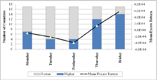
Figure 3 illustrates the results for day of the week effects.

Figure 3

Number of Countries with Higher and Lower Daily Returns by Weekday

Overall, the individual coefficients for daily excess returns are not significant, but Figure 3 shows that

mean excess returns tend to be negative and decreasing in the first three days of the week, in most

countries, while excess returns are positive in Thursdays and Fridays, in most countries. The last day

of the week seems to be, in average, the strongest day of the week. However, only five countries

(Finland, Greece, Iceland, Ireland and Norway) have excess mean returns on Fridays which are

5.2. Bootstrap Approach and GARCH Model

To test the robustness of the results presented in section 5.1, bootstrapping can be applied to the OLS

regressions, as Sullivan, Timmermann and White (2001) propose. These authors warn against the

dangers of data mining in the study of calendar effects, claiming that most of the obtained results are

only “chimeras” and the product of data mining. We use the bootstrap command in Stata 10, with

1000 replications, to all the OLS regressions. This methodology executes the OLS regressions 1000

times, bootstrapping the statistics of the i, by re-sampling observations (with replacement) from the

data. Because this is a non-parametric approach, it is not affected by the non-normality of the data.

Additionally, because we know that there are ARCH effects in our sample daily returns, we

re-estimate the models for month and weekday effects using the ARCH command in Stata 10, allowing

for a GARCH(1,1) process, by means of maximum likelihood. In all estimations, both the ARCH term

and the GARCH are significant at the 1% level, confirming that periods of high and low volatility in

the residuals are grouped.

As additional evidence, we compute a Kruskal-Wallis equality-of-populations rank test, by dividing

daily returns in different groups (months or days of the week), and determining if the null hypothesis

that all groups come from the same population. This is similar to a one-way analysis of variance with

the data replaced by their ranks. Because this a non-parametric test, it does not depend on the data

being normally distributed. The null hypothesis (no effects) is rejected in weekday effects for Greece,

Iceland and Poland, and in month effects for Austria, Iceland and Portugal.

Except for the Kruskal-Wallis test, we do not show the obtained results for the bootstrap approach and

GARCH (1,1) directly, to avoid burdensome tables. We choose to report exclusively, in Table 3,

which day of the week effects remain significant, at a level of 5%, for each of the statistical

INSERT TABLE 3

In day of the week effects, the following days/countries are significant in all statistical methodologies:

(i) positive Fridays in Greece, Iceland, Ireland and Norway; (ii) positive Tuesdays in Germany, and

(iii) negative Mondays in Iceland. The GARCH model additionally uncovers: (i) negative Tuesdays in

Poland and Greece; and, (ii) negative Mondays in Greece. Overall, the two countries who reveal a

stronger day of the week effect are clearly Iceland and Greece, consistently with the weekend effect

extensively documented in the literature. Nevertheless, our overall results are very clear in

demonstrating that there is no across-the-board weekend effect in European stock markets, as in most

countries it is non-existing (including Austria, Denmark, France, Hungary, Italy, Poland, Portugal,

Spain, Switzerland and United Kingdom).

Table 4 reports on month effects detected by all the statistical methodologies applied.

INSERT TABLE 4

As in day of the week effects, we find no overall effect covering the full spectrum of countries under

study, as there are no month effects in Denmark, Finland, Ireland and UK, and the effects initially

detected in some countries do not resist to more robust statistical methodologies, such as France,

Hungary, Italy, Netherlands, Norway, Poland, Spain and Switzerland. On the other hand, the stronger

month effects include: (i) Iceland has positive excess returns in August, and negative in October; (ii)

Austria has positive excess returns in February and negative in September; (iii) Portugal has positive

excess returns in January, and negative in May; and, (iv) Greece has negative excess returns in June.

In our sample, Iceland is clearly the country with stronger calendar effects, revealed both on days of

5.3. Time-stability of day of the week and month effects

Our sample covers a period of fourteen years, between 1994 and 2007. As an additional robustness

check, we investigate if the calendar effects detected are stable, over the whole period under analysis.

It may be the case that the global result is affected by short-run phenomena, in only a few of the years

under study. The purpose of this section is to shed some light on this.

To test the time stability of the coefficients, we compute rolling window OLS regressions on the most

significant coefficients detected in day of the week and monthly effects, both for positive and negative

excess returns. We choose four cases: (i) for positive day of the week: Greece/Friday; (ii) for negative

day of the week: Iceland/Monday; (iii) for positive month: Portugal/ January; (iv) and for negative

month: Iceland/October. In the rolling window OLS regressions, we use a window size of 1000

observations (roughly equivalent to four or five years of observations), and a step size of 200

observations. This means that the first regression uses observations [1;1000], the second regression

uses observations [201;1200] and so on. Given the number of observations available, we compute 14

rolling regressions for each coefficient. In Figure 4, we show the evolution of the i coefficients for

these four strong calendar effects, and also the upper and lower bounds on its 95% confidence interval.

Figure 4

In all four cases, the coefficient that captures the calendar effect fluctuates significantly, as the

windows of observations evolve. In the case of Iceland/October, the coefficient becomes positive both

in the 9th and 10th regression, decreasing again sharply after that. In more than half the regressions, the

upper bound on the 95% confidence interval is a positive return. In the case of Portugal, the January

effect seems to be due mainly to the observations in the first years in the sample, as the effect wears

out in the last eight windows of observations. In the case of Greece, the Friday effect changes radically

from window to window, with periods of higher returns shortly followed by periods of lower returns.

It is only in the last window that the lower bound of the confidence interval is clearly positive. Finally,

the Monday effect in Iceland seems to be only a recent phenomenon, as it did not exist in the first

windows of observations.

Taken together with the results of the previous sections, this evidence of high instability of the

calendar effects coefficients casts further doubt on the significance of the month and day of the week

effects in European stock markets.

6. Conclusions

There is an extensive body of research documenting day of the week and month of the year effects,

particularly in US markets, although international evidence is constantly growing, but with mixed

become weaker in more recent years, both in developing and developed markets. Is it the case that

markets are becoming more efficient and calendar effects are being arbitraged away, or is it the case

that more recent and more powerful statistical methodologies no longer detect those effects, casting

doubt on previous studies?

There is more than one reason why the findings of previous studies may need to be re-assessed. First,

as we discuss in section 4 of this paper, model specifications may have been inadequate for the

detection of calendar effects, in particular the use of t-tests on models with multiple dummy variables.

Second, given the non-normality and other problems in the data, the use of linear regressions may

have lead to the incorrect rejection of the null hypothesis of no calendar effects. Third, a large number

of studies cover only one country or only a few countries, causing some authors to assign a

disproportionate importance to a specific detected effect, which may well be a spurious result

delivered by intensive data mining. Studies covering a large number of countries help authors to

maintain a skeptical point-of-view on country-specific effects, and these types of studies are still in

minority. Fourth, markets develop over time, and widespread knowledge of some types of calendar

effects may have lead to their exploitation by arbitrageurs, thus eroding such effects. So, investigators

need to look at new and more recent data, frequently enough, and to keep checking the time-stability

of previous results.

In our study, we apply robust statistical methodologies and consider only the calendar effects that are

significant under all alternative methodologies. Our main findings are the following.

First, we find no strong convincing evidence of an across-the-board calendar effect in West and

Central European countries. In particular, there are no statistically significant across-the-board January

effects or weekend effects. European countries seem to be mostly immune to day of the week effects,

even though the group of seventeen countries, taken together, does tend to show higher daily returns

calendar effect that warrants further investigation is the general tendency for lower returns in the

holiday months of August and September. All the calendar effects are basically country-specific.

Second, the number of significant coefficients we detect is very similar to the number we would

expect to find in random data. Even though there is some concentration on specific months / days of

the week, our results are not immune to the critique that the calendar effects we detect are exclusively

a result from intensive data mining. This skeptical view is reinforced by the fact that the statistically

stronger calendar effects are not stable over time. In fact, when we use different sub-samples of the

data, the stronger calendar effects that we detect in the whole sample, are not detected in several of

those sub-samples. So, some of the apparently stronger calendar effects may well not be the result of

economic motives, market microstructure, or behavioral traits, but may rather be only lucky snapshots

of capricious movements in the stock market indexes.

Finally, we suggest as avenues for further research, the following. First, some preliminary results we

obtain on day of the month effects, which we do not report, signal that this may be the type of calendar

effect more relevant in European countries, justifying specific research. Second, the use of data on

firms instead of indexes, allows the study of calendar effects by firm characteristics. Third, we need

more studies using broader sets of countries, to determine if calendar effects are across-the-board or

only country-specific. Fourth, a closer look at the low August / September returns in Europe, and the

study of the reasons behind that effect, if it is confirmed. Fifth, there are several alternative variants of

the GARCH model, like TGARCH and IGARCH; which one fits the data better? Sixth, we need to

improve on the microeconomics of calendar effects. We should strive to find the true economic (or

behavioral) rationale behind calendar effects. We need to a better understanding on why calendar

effects are expected to exist, and under what circumstances.

References

Basher, S. and P. Sadorsky “Day of the Week Effects in Emerging Stock Markets”, Applied Economic Letters, 13, 2006, pp. 621-628.

Bollerslev, T. “Generalized Autoregressive Conditional Heteroskedasticity”, Journal of Econometrics, 31, 1986, pp.307-327.

Brooks, C. and G. Persand “Seasonality in Southeast Asian Stock Markets: Some New Evidence on Day of the Week Effects, Applied Economic Letters, 8, 2001, pp. 155-158.

Brown, P., D. Keim, A. Kleidon and T. Marsh “New Evidence on the Nature of Size-related Anomalies in Stock Prices”, Journal of Financial Economics, 12, 1983, pp.33-56.

Chang, E., J. Pinegar and R. Ravichandran “International Evidence on the Robustness of the Day of the Week Effect”, Journal of Financial and Quantitative Analysis, 28, 1993, pp 497-513.

Chen, G., C. Kwok and O. Rui, “The Day of the Week Regularity in the Stock Markets of China”, Journal of Multinational Financial Management, 11, 2001, pp. 139-163.

Choudhry, T. “Day of the Week Effect in Emerging Asian Stock Markets: Evidence from the GARGH Model”,

Journal of Financial Economics, 10, 2000, pp. 235-242.

Chukwuogor-Ndu, C. “Stock Market Returns Analysis, Day of the Week Effect, Volatility of Returns: Evidence from European Financial Markets 1997-2004”, International Research Journal of Finance and Economics, 1, 2006, pp. 112-124

Condoyanni, L., J. O’Hanlon, and C. Ward “Day of the Week Effect on the Stock Returns: International Evidence”, Journal of Business Finance and Accounting, 14, 1987, pp. 159-174.

Connolly, R. “An Examination of the Robustness of the Weekend Effect”, Journal of Financial and Quantitative Analysis, 24, 1989, pp. 133-169.

Connolly, R. “A Posterior Odds Analysis of the Weekend Effect”, Journal of Econometrics, 49, 1991, pp. 51-104.

Cooper, M., J. McConnell and A. Octchinnikov “The Other January Effect”, Journal of Financial Economics, 82, 2006, pp. 315-341.

Cross, F. “The Behavior of Stock Prices on Fridays and Mondays”, Financial Analysts Journal, 29, 1973, pp. 67-69.

Dyl, E. “Capital Gains Taxation and Year-end Stock Market Behavior, Journal of Finance, 32, 1977, pp. 165-175.

Dubois, M. and P. Louvet “The Day of the Week Effect: The International Evidence”, Journal of Banking and Finance, 20, 1996, pp. 1463-1485.

Engle, R. “Autoregressive Conditional Heteroskedasticity with Estimates of the Variance of UK Inflation”,

Econometrica, 50, 1982, pp. 987-1008.

Fama, E. “The Behavior of Stock Prices”, Journal of Business, 38, 1965, pp. 34-105.

French, K. “Stock Returns and the Weekend Effect”, Journal of Financial Economics, 8, 1980. pp. 55-80.

Gibbons, M. and P. Hess “Day of the Week Effects and Asset Returns”, Journal of Business, 54, 1981, pp. 579-596.

Ho, Y., “Stock Return Seasonalities in Asia Pacific Markets”, Journal of International Financial Management and Accounting, 2, 1990, pp. 47-77.

Hui, T. “Day of the Week Effects in US and Asia-Pacific Stock Markets During the Asian Financial Crisis: a Non-parametric Approach”, The International Journal of Management Science, 33, 2005, pp. 277-282.

Jaffe, J. and R. Westerfield “The Weekend Effect in Stock Returns: the International Evidence”, Journal of Finance, 41, 1985a, pp. 433-454.

Jaffe, J. and R. Westerfield “Patterns in Japanese Common Stock Returns: The International Evidence”, Journal of Financial and Quantitative Analysis, 20, 1985b, pp. 243-260.

Kamara, A. “New Evidence on the Monday Seasonal in Stock Returns”, Journal of Business, 70, 1997, pp. 63-84.

Keim, D. “Size Related Anomalies and Stock Return Seasonality: Further Empirical Evidence”, Journal of Financial Economics, 12, 1983, pp. 12-32.

Keim, D. and R. Stambaugh “A Further Investigation of the Weekend Effect in Stock Returns. Journal of Finance, 39, 1984, pp. 819-835.

Kim, D. and S. Kon “Alternative Models for the Conditional Heterocedasticity of Stock Returns”, Journal of Business, 67, 1994, pp. 563-598.

Kohers, G., N. Kohers, V. Pandey and T. Kohers “The Disappearing Day of the Week Effect in the World’s Largest Equity Markets”, Applied Economic Letters, 11, 2004, pp. 167-171.

Lau, A., H. Lau and J. Wingender “The Distribution of Stock Returns: New Evidence Against the Stable Model”, Journal of Business and Economic Statistics, 8, 1990, pp. 217-223.

Maberly, E. and D. Waggoner, “Closing the Question on the Continuation of the Turn of the Month Effects: Evidence from the S&P 500 Index Future Contracts”, Federal Reserve Bank of Atlanta, 2000.

Menyah, K. “New Evidence on the Impact of Size and Taxation on the Seasonality of UK Equity Returns”,

Review of Financial Economics, 8, 1999, pp.11-25.

Officer, R. “Seasonality in Australian Capital Markets: Market Efficiency and Empirical Issues”, Journal of Financial Economics, 2, 1975, pp. 29-52.

Reinganum, M. “The Anomalous Stock Market Behavior of Small Firms in January: Empirical Tests for Tax-Loss Effects”, Journal of Financial Economics, 12, 1983, pp. 89-104.

Rogalski, R “New Findings Regarding Day of the Week over Trading and Non-trading Periods: a Note, Journal of Finance, 39, 1984, pp. 1903-1614.

Rosenberg, M “The Monthly Effect in Stock Returns and Conditional Heteroskedasticity”, American Economist, 48, 2004, pp. 67-73.

Rozeff, M. and W. Kinney, “Capital Market Seasonality: The Case of Stock returns”, Journal of Financial Economics, 3, 1976, pp. 379-402.

Rubinstein, M. “Rational Markets: Yes or No? The Affirmative Case”, Financial Analysts Journal, 57, 2001, pp. 15-29.

Schwert, G. “Anomalies and Market Efficiency”, in G. Constantinides et al., Handbook of the Economics of Finance, 2001, North Holland, Amsterdam.

Steely, J. “A Note on Information Seasonality and the Disappearance of the weekend Effect in UK Stock Market”, Journal of Banking and Finance, 25, 2001, pp. 1941-1956.

Sullivan, R., A. Timmermann, and H. White, ”Dangers of Data mining: The Case of Calendar Effects in Stock Returns”, Journal of Econometrics, 105, 2001, pp. 249-286.

Tonchev, D. and T. Kim “Calendar Effects in Eastern European Financial Markets: Evidence from the Czech Republic, Slovakia and Slovenia”, Applied Financial Economics, 14, 2004, pp. 1035-1043.

Table 1

Descriptive Statistics for Daily Returns (1994-2007)

Country Index

Observa-tions Mean

Standard Deviation

Standard Error of

Mean

Maximum Minimum 10

th

Percentile

90th

Percentile Skewness Kurtosis

Table 2 (a)

Differences in Mean Returns: Month Effects and Day of the Week Effects (1994-2007)

Austria Denmark Finland France Germany Greece Hungary Iceland Ireland Month Effects

January (m1) 0.0008370 0.0006718 -0.0000672 0.0004758 0.0004642 0.0012756 0.0030919*** 0.0014591*** 0.0005312

February (m2) 0.0012117* 0.0000033 -0.0005953 -0.0003238 -0.0001027 0.0000724 -0.0006621 0.0006754 0.0001269

March (m3) -0.0001552 -0.0004547 -0.0001447 0.0005065 0.0000163 -0.0003734 -0.0005116 -0.0001510 -0.0001220

April (m4) 0.0011506* -0.0000662 0.0019942 0.0013475 0.0008637 0.0012275 0.0007798 0.0000061 0.0003006

May (m5) -0.0002729 0.0000892 -0.0016483 -0.0009067 -0.0005842 -0.0003769 -0.0014368 -0.0005309 -0.000579

June (m6) -0.0002558 -0.0002900 -0.0003972 -0.0002228 0.0003801 -0.0018381** 0.0001130 -0.0002897 -0.0003666

July (m7) -0.0002316 0.0004002 -0.0006373 -0.0005493 0.0000795 0.0011410 0.0006777 -0.0000392 -0.0005222

August (m8) -0.0009997 -0.0000412 -0.001093 -0.0012453 -0.0015085* -0.0008802 -0.0010083 0.0012296*** -0.0000880

September (m9) -0.0014473** -0.0011481* -0.0003406 -0.0019372** -0.0023202*** -0.0002694 -0.0017642* -0.0003333 -0.0010632*

October (m10) -0.0009800* 0.0000347 0.0017162 0.0012442 0.0006597 -0.0009277 -0.0001182 -0.0010512** 0.0004554

November (m11) 0.0004969 0.0004069 0.0015542 0.0011597 0.0018291** 0.0003771 -0.0007940 -0.0010134** 0.0006287

December (m12) 0.0010656* 0.0004432 -0.0004157 0.0005599 0.0004149 0.0006386 0.0019474* 0.0001833 0.0008309

Weekday Effects

Monday (d1) 0.0003267 0.0002133 0.0003584 -0.0001953 0.0001200 -0.0011393* 0.0010105 -0.0010800*** -0.0007305*

Tuesday (d2) -0.0000216 -0.0001378 -0.0013173 0.0001918 0.0012919** -0.0009483 -0.0002630 -0.0002404 -0.0000191

Wednesday (d3) -0.0005173 0.0000549 -0.0010811 -0.0003940 -0.0002125 0.0002494 -0.0006958 -0.0003118 -0.0002824

Thursday (d4) 0.0007971* 0.0001466 0.0004348 0.0000647 -0.0006418 0.0002865 -0.0009669 0.0004697 0.0001105

Friday (d5) -0.0005772 -0.0002778 0.0016806** 0.0003375 -0.0005415 0.0015450** 0.0009558 0.0011560*** 0.0008772**

Table 2 (b)

Differences in Mean Returns: Month Effects and Day of the Week Effects (1994-2007)

Italy Netherlands Norway Poland Portugal Spain Switzerland UK Month Effect

January (m1) 0.0012869* -0.0003875 0.0006695 0.0023601** 0.0018092*** 0.0002735 -0.0004143 -0.0004209

February (m2) -0.0001054 0.0002576 -0.0000159 0.0010675 0.0008848* 0.0008105 -0.0002606 0.0000201

March (m3) 0.0005654 -0.0004310 -0.0000091 -0.0006989 -0.0000436 -0.0007650 0.0003083 -0.0000293

April (m4) 0.0009929 0.0013887 0.0010869 0.0009733 -0.0006660 0.0009011 0.0009134 0.0007768

May (m5) -0.0013138* -0.0002559 -0.0002246 -0.0020804* -0.0011030* -0.0003470 0.0000091 -0.0005743

June (m6) -0.0008792 -0.0001735 0.0000732 -0.0000233 -0.0008001 -0.0006307 0.0000303 -0.0005211

July (m7) -0.0001825 -0.0000570 0.0003118 0.0007452 -0.0002300 -0.0007125 -0.0004382 0.0000865

August (m8) -0.0009048 -0.0007284 -0.0009551 -0.0002820 -0.0009143 -0.0011146 -0.0012106* -0.0002095

September (m9) -0.0012298* -0.0020503** -0.0018248*** -0.0016862 -0.0012040** -0.0009877 -0.0010732 -0.0009836

October (m10) -0.0001614 0.0008677 0.0004716 -0.0002076 0.0008932 0.0008898 0.0007582 0.0008577

November (m11) 0.0014259* 0.0011520 0.0002235 -0.0002220 0.0007718 0.0016059** 0.0012480* 0.0004334

December (m12) 0.0007903 0.0006395 0.0003714 0.0008053 0.0006780 0.0003548 0.0002129 0.0005978

Weekday Effect

Monday (d1) -0.0005973 0.0005714 -0.0001770 0.0008422 -0.0003908 -0.0006186 -0.0000761 -0.0000452

Tuesday (d2) 0.0000217 -0.0001557 -0.0004651 -0.0016038** -0.0000050 0.0002262 -0.0001401 -0.0001057

Wednesday (d3) -0.0003295 -0.0004713 -0.0007308 -0.0010887 0.0001411 -0.0005240 0.0000865 -0.0005845

Thursday (d4) 0.0002900 -0.0003432 0.0004058 0.0012438* -0.0001887 0.0000621 -0.0001172 0.0001690

Friday (d5) 0.0006044 0.0004175 0.0009807** 0.0007086 0.0004365 0.0008570* 0.0002453 0.0005648

Table 3

Weekday Effects by Country (At Significance Level: 5%)

Country Index Higher Returns than Other Weekdays Lower Returns than Other Weekdays

Kruskal – Wallis Test Regression Bootstrap

/Regression

GARCH

Model Regression

Bootstrap /Regression

GARCH Model

Austria ATX - - - 0.3485

Denmark OMXC20 - - - 0.9661

Finland OMXHPI Friday* Friday* - - - - 0.1232

France CAC40 - - - 0.9454

Germany DAX Tuesday* Tuesday* Tuesday* - - - 0.1189

Greece ASE Friday* Friday** Friday** - - Mon**, Tue** 0.0005**

Hungary BUX - - - _0.2635

Iceland OMXIPI Friday** Friday** Friday** Monday* Monday** Monday** 0.0001**

Ireland ISEQ Friday* Friday* Friday* - - - 0.1305

Italy MIBTEL - - - 0.3035

Netherlands AEX - - - 0.2455

Norway OSEAX Friday* Friday* Friday* - - - _0.0507

Poland WIG - - - Tuesday* - Tuesday* 0.0302*

Portugal PSI20 - - - 0.8178

Spain IBEX - - - 0.2686

Switzerland SMI - - - 0.9568

UK FTSE - - - 0.2400

Table 4

Month Effects by Country (At Significance Level: 5%)

Country Index Higher Returns than Other Months Lower Returns than Other Months

Kruskal – Wallis Test Regression Bootstrap

/Regression

GARCH

Model Regression

Bootstrap /Regression

GARCH Model

Austria ATX - Feb*, Apr* Feb* Sep* Sep* Sep** 0.0383*

Denmark OMXC20 - - - 0.9791

Finland OMXHPI - - - 0.7046

France CAC40 - - - Sep* - - 0.4088

Germany DAX Nov* Nov* - Sep** Sep* - _0.5714

Greece ASE - - - Jun* Jun* Jun* 0.2311

Hungary BUX Jan** Jan* - - - - 0.0744

Iceland OMXIPI Jan**, Aug** Jan**, Aug** Aug** Oct*, Nov* Oct*, Nov* Oct* 0.0012**

Ireland ISEQ - - - _0.6429

Italy MIBTEL - Nov* - - - - 0.0847

Netherlands AEX - - - Sep** Sep* - 0.5963

Norway OSEAX - - - Sep** Sep* - 0.5902

Poland WIG Jan* Jan* - - - - 0.1285

Portugal PSI20 Jan** Jan** Jan** Sep* May* May* 0.0180*

Spain IBEX Nov* Nov* - - - - 0.3301

Switzerland SMI - Nov* - - - - 0.6630

UK FTSE - - - 0.7609